Mar 1, 1999 - KEY WORDS: Normal quantile (scores) plots; t-distribution confidence interval for a mean; robustness; test of normality; lognormal, Cauchy, and ...
Normal Quantile Plots and Statistical Inference Robert L. Wardrop March 1, 1999
Abstract A number of statistics texts contain the advice, “For a small sample, if the data look normal you may use the t-distribution to obtain a confidence interval for the population mean.” This paper indicates that this advice is incorrect. More precisely, for a particular skewed population (a lognormal) it is shown that the advice is backwards: the confidence interval performs much worse for data that look normal than it does for data that do not look normal! Further, it is argued that this finding should be true for other skewed populations. It is shown that the advice is wrong for the symmetric double exponential or Cauchy population. Finally, for normal populations the advice might be irrelevant: the performance of the confidence interval does not seem to depend on the appearance of the data. KEY WORDS: Normal quantile (scores) plots; t-distribution confidence interval for a mean; robustness; test of normality; lognormal, Cauchy, and double exponential distributions.
1
1 Introduction In a typical first course in Statistics, the student learns that if a researcher selects a random sample of size n from a normal population, then the t-distribution can be used to obtain an exact confidence interval for the √ mean. The confidence interval formula can be written as x ¯ ± ts/ n, where x ¯ is the mean of the data, s is the standard deviation of the data, and t is obtained from the t-distribution with (n − 1) degrees of freedom. Now this is a fine, some might say beautiful, mathematical result. But its practical value is uncertain to the student; in “real life” there is nobody to tell a researcher whether the population is normal. The serious student is left to wonder: Is the t-distribution confidence interval simply (another) useless mathematical result or is it, somehow, more applicable than the above statement suggests? Many introductory textbooks ignore the serious student’s question, but some of the better textbooks try to deal with it. In particular, several books encourage the student to “look at the data.” For example, if the sample size is less than 15, Moore and McCabe (1989), p. 520, advise their readers to • Use t procedures if the data are close to normal. If the data are clearly nonnormal or if outliers are present, do not use t. Further, Moore and McCabe suggest that a normal quantile plot (or a normal scores plot) is a good way to determine whether data are close to normal. It is difficult to find fault with the spirit of this advice. I certainly prefer to have a student thinking rather than mindlessly depending on somebody else’s specification of the true assumptions. Unfortunately, however, as I argue below, this advice is wrong. In fact, it is more than simply wrong; it is, in a sense, backwards, as demonstrated below. I have found variations on the above advice in several texts, but what surprises me is that none of the texts contains a justification for the advice or a reference to a published justification of it. My best conjecture is that the advice is something that “All sensible people know must be true.” It is curious, however, that a statistician would embrace this advice. The sampling theory approach to statistics requires that one considers not just the data actually obtained, but all the data that could have been obtained. One can embrace the above advice, however, only if one believes that the single realization (the data actually collected) conclusively reveals the nature of the skewness of the population. As we will see below the advice is wrong because it misdirects the student’s thinking from what is important, the population, to what is relatively unimportant in this case, the data.
2 An Unexpected Result Figure 1 presents the lognormal pdf with parameters 5 and 1. (This means that if X has the pictured pdf, then the natural log of X has the normal distribution with mean 5 and standard deviation 1.) In this paper, “lognormal” always will mean the lognormal distribution with parameters 5 and 1. This pdf is strongly skewed to the right and one would suspect that the t-distribution confidence interval for the mean is not very robust for a small sample. This suspicion is correct. I performed a 10,000 run simulation experiment to estimate the actual coverage probability for the tdistribution confidence interval for the population mean when the sample size equals 10. The results are in Table 1. The performance of the t-distribution confidence interval is quite poor. For example, the actual coverage probability of the nominal 95 percent interval is approximately 83 to 84 percent. I will now examine the advice for random samples of size 10 from the lognormal. I need to operationalize what it means for data to “look normal.” Looney and Gulledge (1985) suggest using the correlation coefficient of the normal scores plot to perform a formal test of the (null) hypothesis that the population
2
is a normal curve, and they provide critical values for a variety of sample sizes. I will use the correlation coefficient of the normal scores plot to decide whether the data look normal. In addition to obtaining the confidence interval for the mean, for each run of my simulation experiment I computed the correlation coefficient for the normal scores plot and determined whether the null hypothesis of normality would be rejected by the Looney and Gulledge test. The test was performed twice, for type one error α = 0.05 and 0.10. Then I created the cross-tabulation of the result of the test of normality (reject or not) and the performance of the confidence interval (correct or not). For example, for α = 0.05 and a nominal confidence level of 80 percent, I obtained the results shown in Table 2. First, consider the marginal totals. Note that 70.31 percent of the simulated intervals were correct, in agreement with the value in Table 1. Also, note that the estimated power of the Looney and Gulledge test is 0.5901 (with α = 0.10, the estimated power is 0.6888). Next, note that the point estimate of the probability the interval is correct given normality is rejected equals 4,777/5,901= 0.8095, and the point estimate of the probability the interval is correct given normality is not rejected equals 2,254/4,099 = 0.5499. In words, the confidence interval performs as desired when the data do not look normal and its performance is abysmal when the data look normal. This result is the exact opposite of what one would expect if the earlier advice was valid! The above computations were repeated for the remaining seven combinations of nominal confidence level and α. The results are presented in Table 3. Note the following features revealed by this table. 1. The example immediately above appears at the bottom left of the table. For a nominal error rate of 20 percent (nominal confidence level of 80 percent), and α = 0.05 in the test of normality, the estimated error rate given that the normality is rejected is considerably smaller than the estimated error rate given that normality is not rejected. This pattern is repeated in the other seven combinations of nominal level and α. 2. For each nominal level, both error rates increase somewhat as α is changed from 0.05 to 0.10. 3. With the exception of the case with 20 percent nominal error rate, and normality rejected with α = 0.05, all estimated error rates exceed their nominal values.
3 Why? Why am I getting this bizarre result? Why is it that the t-distribution performs worse when the data look normal? Let us consider my simulation experiment again. From Table 1, for the nominal 95 percent confidence interval, 1,647 of the simulated intervals were incorrect; that is, they did not contain the population mean 244.7. Only five of the incorrect intervals were too large (left endpoint larger than 244.7), and 1,642 were too small! √ The confidence interval will be too large for the population mean if x ¯ − ts/ n > µ. Thus, intuitively, the data must have a large mean, but a relatively small standard deviation. The mean becomes larger by having either more observations in the right tail or one or more observations far out in the tail. But either of these conditions will tend to inflate the standard deviation, making it more difficult for the confidence interval to be too large. One way for an interval to be too small is for all of the observations in the data set to be small (that is, no observations in the tail). This is not an unlikely occurrence. For example, a simple computation verifies that the probability is 11.4 percent that all ten of the observations from the lognormal will be 350 or smaller. Look at Figure 1 again. Conditional on all observations being smaller than, say, 350, we are sampling from a pdf that might be difficult to distinguish from a normal pdf with a sample of size 10. 3
Unfortunately, when I performed my simulation study I neglected to determine the maximum of each simulated data set. Therefore, I performed an additional small study in which I simulated random samples of size 10 from the lognormal until I had 100 data sets for which the maximum observation did not exceed 350. These 100 data sets looked normal: normality was rejected at α = 0.05 for only 10 data sets, and was rejected at α = 0.10 for only 21 data sets (compared to 59 and 69 percent, respectively, for the original simulation study). In addition, 92 of the 100 intervals were incorrect. (The eight correct intervals were among the 79 data sets for which normality was not rejected for either α.)
4 More Examples I will repeat the analysis of Section 2 for random samples of size 20 from the lognormal. The first result is that the confidence interval based on the t-distribution is not very robust. The point estimates plus or minus two estimated standard errors of the coverage probabilities are: 0.7364 ± 0.0088, 0.8178 ± 0.0077, 0.8655 ± 0.0068, and 0.9241 ± 0.0053 for the nominal 80, 90, 95, and 99 percent intervals, respectively. (Note: The lognormal provides a good counterexample to another bit of advice in Moore and McCabe (1989), p. 520, namely “The t procedures can be used even for clearly skewed distributions when the sample is large, roughly n ≥ 40.” In fact, for n as large as 200, the t-distribution confidence interval is not very robust. See Wardrop 1995, p. 561.) Second, the power of the test of normality is very high. In particular, the estimated power is 0.9158 ±0.0056 for α = 0.05, and is 0.9498 ±0.0056 for α = 0.10. Therefore, the conditioning argument is not as interesting as it was earlier. It is still true that given the data look normal, the confidence interval performs far worse than if the data do not look normal. But the practical implications of this fact are diminished because the data so rarely look normal! Table 4 is the analogue of Table 3 for the current situation. The patterns noted in the earlier table are repeated, except that in the current setting all point estimates exceed the nominal error rates. I suppose that one could repeat my analyses for other skewed distributions, but I will not do so. I am convinced that the above results will persist for other skewed distributions because, roughly speaking: • The data will look most like normal whenever the tail is not represented in the data, and with no data in the tail the interval likely will be too small. • The data will look least like normal whenever the tail is represented in the data, and with data in the tail the interval likely will be correct. I do not expect my musings to convince all readers; thus, somebody might want to research this topic. Instead, I will repeat the above analyses for random samples of size 10 from the double exponential, Cauchy, and normal distributions. I will begin with the double exponential. The t-distribution interval is quite robust. The point estimates plus or minus two estimated standard errors of the coverage probabilities are: 0.7943 ± 0.0081, 0.9036 ± 0.0059, 0.9589 ± 0.0040, and 0.9940 ± 0.0015 for the nominal 80, 90, 95, and 99 percent intervals, respectively. In fact, for the 95 and 99 percent levels, the actual coverage probabilities appear to exceed the nominal values. Not surprisingly, the test of normality has little power for a sample of size 10; the estimates are 0.2661 ± 0.0088 for α = 0.10, and 0.1791 ± 0.0077 for α = 0.05. Table 5 presents estimated error rates for the eight combinations of nominal level and α. Please note the following. 4
1. Of the 1,791 runs for a nominal error rate of 0.01, α = 0.05, and normality rejected, only two of the confidence intervals were incorrect. As a result, twice the estimated standard error (0.0016) is larger than the point estimate (0.0011). 2. As before, the estimated error rate when the data do not look normal is lower than when they look normal. The difference between the error rates decreases as the nominal confidence level decreases; for the 80 percent nominal confidence level, the two error rates are not importantly different. For the Cauchy, the t-distribution interval has an actual coverage that exceeds the nominal level. This is not surprising, because the impact of the heavy tails of the Cauchy will be larger on s than on x ¯, leading to intervals that are too wide, and, hence, have too high a probability of coverage. The point estimates plus or minus two estimated standard errors of the coverage probabilities are: 0.8265 ± 0.0076, 0.9402 ± 0.0047, 0.9793 ± 0.0028, and 0.9984 ± 0.0008 for the nominal 80, 90, 95, and 99 percent intervals, respectively. The test of normality has approximately the same power for a Cauchy alternative as it did for the lognormal. The estimates are 0.6881 ± 0.0093 for α = 0.10, and 0.6188 ± 0.0097 for α = 0.05. Table 6 presents estimated error rates for the eight combinations of nominal level and α. Please note the following. 1. Only 16 of the nominal 99 percent confidence intervals were incorrect. While it is clear that the error rate for data that do not look normal is lower than the error rate for data that look normal, neither of these extremely small error rates is estimated very satisfactorily. 2. The estimated error rate when the data do not look normal is lower than when they look normal. Finally, I simulated samples from a normal population. I will suppress the details, but the simulation came out correct: the estimated coverage probabilities are not different from the nominal levels, and neither probability of rejecting normality is different from its α. You may interpret this as verifying that Gosset, and Looney and Gulledge were correct, or, more reasonably, that my simulation was not obviously flawed. Table 7 presents estimated error rates for the eight combinations of nominal level and α. Please note the following. 1. For 80, 90, and 95 percent confidence levels, the error rate for data that look normal is not different from the error rate for data that do not look normal. For the 99 percent level, the point estimates (finally) give some support to the advice, but the differences are not statistically significant. 2. In words, if your population is normal, the advice is still wrong; the t-interval works fine even when the data do not look normal. But there is a small vindication for advocates of the advice; we finally have a situation in which data that do not look normal do not outperform data that look normal!
5 A Positive Conclusion My interpretation of this paper is that it provides another example of why science is important in Statistics. In general, the better a statistician understands the scientific problem being studied, the better will be the statistical analysis. The advice pretends that the science behind the data does not matter. The advice says, “It does not matter whether these 10 numbers measure anxiety or yield or survival times. Simply by looking at the numbers I can tell whether I should use the t-distribution.” To be sure, there may be times when even the most knowledgeable scientist will be uncertain as to whether the population is severely skewed, and, therefore, uncertain whether the t-distribution should be 5
used for a small sample. Statisticians have developed many clever ways to measure uncertainty in a huge variety of settings; we should remember that it is important to recognize those situations in which we have uncertainty that we do not know how to measure, such as the uncertainty of how the t-distribution will perform in a poorly understood scientific problem. References Looney, S. W., and Gulledge, T. R. Jr. (1985), “Use of the Correlation Coefficient with Normal Probability Plots,” The American Statistician, 39, 75–79. Moore, D. S., and McCabe, G. P. (1989), Introduction to the Practice of Statistics, New York: W. H. Freeman and Company. Wardrop, R. L. (1995), Statistics: Learning in the Presence of Variation, Dubuque, Iowa: Wm. C. Brown Publishers.
6
...... .. ........ .... ... .... ... ... ... ... ... .... . ..... 0.002 .. ...... .. ........ .. ........... .................... ... ....... . µ = 244.7 100 500 0.004
Figure 1: The lognormal pdf.
Table 1: Estimates of true coverage probability when using the t-distribution confidence interval, the population is lognormal, and the sample size is 10. Nominal Confidence Level 80% 90% 95% 99%
ˆ Estimate ±2 SE 0.7031 ± 0.0091 0.7860 ± 0.0082 0.8353 ± 0.0074 0.9036 ± 0.0059
Table 2: Cross-tabulation of the results of the confidence interval and the test of normality, for 80 percent nominal confidence and α = 0.05. Normality? Conf. Int. Rejected Not Rejected Total Correct 4,777 2,254 7,031 Incorrect 1,124 1,845 2,969 Total 5,901 4,099 10,000
7
Table 3: Estimated error rate (± two estimated standard errors) of the t-distribution confidence interval for a random sample of size 10 from the lognormal. The test of normality is conducted at two levels, α = 0.05 and α = 0.10. Estimates are based on a total of 10,000 runs of a simulation experiment. Normality? Rejected Not Rejected
Nominal Error Rate = 0.01 α = 0.05 α = 0.10 0.0393 ± 0.0051 0.0495 ± 0.0052 0.1786 ± 0.0120 0.2002 ± 0.0143
Normality? Rejected Not Rejected
Nominal Error Rate = 0.05 α = 0.05 α = 0.10 0.0869 ± 0.0073 0.1003 ± 0.0072 0.2767 ± 0.0140 0.3072 ± 0.0165
Normality? Rejected Not Rejected
Nominal Error Rate = 0.10 α = 0.05 α = 0.10 0.1220 ± 0.0085 0.1368 ± 0.0083 0.3464 ± 0.0149 0.3850 ± 0.0174
Normality? Rejected Not Rejected
Nominal Error Rate = 0.20 α = 0.05 α = 0.10 0.1905 ± 0.0102 0.2115 ± 0.0098 0.4501 ± 0.0155 0.4859 ± 0.0179
Table 4: Estimated error rate (± two estimated standard errors) of the t-distribution confidence interval for a random sample of size 20 from the lognormal. The test of normality is conducted at two levels, α = 0.05 and α = 0.10. Estimates are based on a total of 10,000 runs of a simulation experiment. Normality? Rejected Not Rejected
Nominal Error Rate = 0.01 α = 0.05 α = 0.10 0.0567 ± 0.0048 0.0623 ± 0.0050 0.2850 ± 0.0311 0.3327 ± 0.0421
Normality? Rejected Not Rejected
Nominal Error Rate = 0.05 α = 0.05 α = 0.10 0.1092 ± 0.0065 0.1171 ± 0.0066 0.4097 ± 0.0339 0.4641 ± 0.0445
Normality? Rejected Not Rejected
Nominal Error Rate = 0.10 α = 0.05 α = 0.10 0.1541 ± 0.0075 0.1637 ± 0.0076 0.4881 ± 0.0345 0.5319 ± 0.0445
Normality? Rejected Not Rejected
Nominal Error Rate = 0.20 α = 0.05 α = 0.10 0.2359 ± 0.0089 0.2457 ± 0.0088 0.5653 ± 0.0342 0.6016 ± 0.0437
8
Table 5: Estimated error rate (± two estimated standard errors) of the t-distribution confidence interval for a random sample of size 10 from the double exponential. The test of normality is conducted at two levels, α = 0.05 and α = 0.10. Estimates are based on a total of 10,000 runs of a simulation experiment. Normality? Rejected Not Rejected
Nominal Error Rate = 0.01 α = 0.05 α = 0.10 0.0011 ± 0.0016 0.0023 ± 0.0019 0.0071 ± 0.0019 0.0074 ± 0.0020
Normality? Rejected Not Rejected
Nominal Error Rate = 0.05 α = 0.05 α = 0.10 0.0246 ± 0.0073 0.0293 ± 0.0065 0.0447 ± 0.0046 0.0454 ± 0.0049
Normality? Rejected Not Rejected
Nominal Error Rate = 0.10 α = 0.05 α = 0.10 0.0748 ± 0.0124 0.0838 ± 0.0107 0.1011 ± 0.0067 0.1010 ± 0.0070
Normality? Rejected Not Rejected
Nominal Error Rate = 0.20 α = 0.05 α = 0.10 0.1887 ± 0.0185 0.2018 ± 0.0156 0.2094 ± 0.0090 0.2071 ± 0.0095
Table 6: Estimated error rate (± two estimated standard errors) of the t-distribution confidence interval for a random sample of size 10 from the Cauchy. The test of normality is conducted at two levels, α = 0.05 and α = 0.10. Estimates are based on a total of 10,000 runs of a simulation experiment. Normality? Rejected Not Rejected
Nominal Error Rate = 0.01 α = 0.05 α = 0.10 0.0003 ± 0.0005 0.0006 ± 0.0006 0.0037 ± 0.0020 0.0038 ± 0.0022
Normality? Rejected Not Rejected
Nominal Error Rate = 0.05 α = 0.05 α = 0.10 0.0076 ± 0.0022 0.0103 ± 0.0024 0.0420 ± 0.0065 0.0436 ± 0.0073
Normality? Rejected Not Rejected
Nominal Error Rate = 0.10 α = 0.05 α = 0.10 0.0338 ± 0.0046 0.0394 ± 0.0047 0.1020 ± 0.0098 0.1048 ± 0.0110
Normality? Rejected Not Rejected
Nominal Error Rate = 0.20 α = 0.05 α = 0.10 0.1475 ± 0.0090 0.1533 ± 0.0087 0.2156 ± 0.0133 0.2180 ± 0.0148
9
Table 7: Estimated error rate (± two estimated standard errors) of the t-distribution confidence interval for a random sample of size 10 from the normal. The test of normality is conducted at two levels, α = 0.05 and α = 0.10. Estimates are based on a total of 10,000 runs of a simulation experiment. Normality? Rejected Not Rejected
Nominal Error Rate = 0.01 α = 0.05 α = 0.10 0.0133 ± 0.0100 0.0129 ± 0.0071 0.0094 ± 0.0020 0.0092 ± 0.0020
Normality? Rejected Not Rejected
Nominal Error Rate = 0.05 α = 0.05 α = 0.10 0.0514 ± 0.0193 0.0555 ± 0.0144 0.0491 ± 0.0044 0.0485 ± 0.0045
Normality? Rejected Not Rejected
Nominal Error Rate = 0.10 α = 0.05 α = 0.10 0.0933 ± 0.0254 0.1011 ± 0.0190 0.0959 ± 0.0061 0.0952 ± 0.0062
Normality? Rejected Not Rejected
Nominal Error Rate = 0.20 α = 0.05 α = 0.10 0.1924 ± 0.0344 0.2071 ± 0.0255 0.1954 ± 0.0081 0.1939 ± 0.0083
10