correlations by this test. Therefore. results of the t-test are no substitute for sound geological reasoning. caveat emptor. Introduction. Suppose x i j (i = 1, 2, ... , n, ...
CAN. J . EARTH SCI. VOL. 11, 1974
Note on Closure Correlation ERWINZODROW
Can. J. Earth Sci. Downloaded from www.nrcresearchpress.com by Peking University on 05/28/13 For personal use only.
St. Francis Xavier University, Sydney Campus, P.O. Box 760, Sydney, Nova Scotia BIP 6JI Received April 19,1974 Revision accepted for publication August 20,1974 Given a matrix of product-moment correlation coefficients computed on 'closed data' (a system of percentage variables), the test of departure from zero correlation is clearly inappropriate because closure of data imposes non-zero correlation. Subroutine CHAYES estimates 'Null Correlations' and calculates a t-matrix which may be used to test the hypothesis that observed product-moment correlations are due to the closure property. The calculated t-matrix is at best an approximation. This is found in certain mathematical assumptions leading to this t-test, and the recognition that statistical assumptions in the theory of r-testing are not satisfied. Great care must be exercized in accepting or rejecting correlations by this test. Therefore. results of the t-test are no substitute for sound geological reasoning. caveat emptor.
Introduction Suppose xij (i = 1, 2, ... , n, j = 1, 2, ... , m) is a data matrix X of n samples and m variates. It is common practice in geology to employ observations determined as proportions (percentages) of the variates as input data for statistical analysis. Proportions have this objectionable property: yij = xij/xi, so that y,, equals 1 or 100%. This is the closure property. Even if the x-variates are uncorrelated, the closure effect imposes non-zero correlations p,, on the y-variates. The non-zero correlation is strongly negatively biased. In a recent monograph Chayes (1971, Chap. 1) has evaluated the expection of p,, when the x-variates are uncorrelated, using the usual asymptotic expansion for determining the expected value of a ratio. Chayes proposed using this (expected) value as the null model in a ttest on the observed correlations. Because of the closure property in y, it is statistically inappropriate to employ the test of departure from zero correlation. Doubts about the desirability of using this test were raised by Chayes himself, partly because of uncertainty over the range of data for which the asymptotic approximation is acceptable, and partly because of the advocacy of using the test for all of the individual elements of what could be a large correlation matrix.' 'Currently Grant and Zodrow are investigating the effects on the power of the t"-test by re-evaluating Taylor's expansion. Chayes (1971, p. 9) used expanding powers about zero. We advocate expansion about the Can. J. Earth Sci., 11, 1616-1619(1974)
On the other hand, Chayes has opened an avenue for the study of proportions in statistical algorithms so that we now have at least a measure for testing correlations based on proportions against an appropriately defined null model.
Test of Hypothesis in the Null Model One factor of crucial importance in any test of a hypothesis is the number of samples n, and the associated concepts of power of the test, confidence limits, and efficiency. Our own experiments with random sampling numbers, a matrix of (300, lo), demonstrates these result^:^ mean if it is greater than 118 (about 16%). Expansion of Taylor series (to obtain expectencies) about zero is excellent for trace element correlations. Leibniz' test is used to get upper bounds of errors, since the series expansion of cldless than 1 (the power series) is alternating in sign. For large c/d less than 1, the power of the t"-test is not convincing. 'With the aid of random sampling numbers a (300, 10) data matrix was constructed. The each row in this matrix was converted to percentages to obtain closure. Thus, we are able to work with the t"-test matrix, null correlations, product-moment, and correlations of the random sampling numbers (x-variates). The testing is constructed to examine the t"-test: Error Types I and 11. The percentage quoted (94%) is success (accept the null model, reject it if warranted avoiding Error Types I and 11). Further, this simulation process, carried out for purposes of testing orthopyroxene electron microprobe data, indicates that with decreasing sample size (10 samples as lower n) successes hover about 93 to 99%, with not lower than 90% confidence. Over 1000 correlations were tested in this manner. These tests indicate that a confidence level of 90% is desirable, for with higher limits successes are lowered by either Error Types I or I1 (Zodrow 1974).
1617
Can. J. Earth Sci. Downloaded from www.nrcresearchpress.com by Peking University on 05/28/13 For personal use only.
NOTES
(1) when n = 300, Chayes' t "-test gives excellent results, rejecting or accepting correctly correlations (avoiding Errors Types I and 11). On the other hand, tests for departure from zero correlations show that 90% of the product-moment correlations in y are different from zero (all testing was done at the 0.05 level of significance). (2) With decreasing sampling numbers (n = 50, 20, lo), Chayes' model either rejects or accepts about 94% of the correlations correctly. The power of the conventional null hypothesis improves, but does not measure up to that of the null model. Like all simulations, the results lack generality, but they may be taken as indicators. The range of the input data, and consequently the ranges of the observed averages (j,) must be considered a factor. Another factor of interest in this context is the notion of the ratio of number of variables, rn, to the number of samples, n . Additional problems are encountered since in the expression for the open variance, ai2 (Chayes 1971, p. 46, e.g. 5-3) negative values are permissible. Algebraically, this does not pose problems. But the test for closure must, in this situation, be regarded as impossible. It can be construed as a crude group test to reject the hypothesis of closure correlations. It should also be noted that the test is inappropriate unless rn is greater than or equal to 4 (if rn is 2, Eq. [I] becomes infinity; if rn is 3, the closure hypothesis is trivially accepted). Since Pi equals the probability of x i in X, it is interesting to speculate under what conditions the open variance (oi2) equals the observed variance from the data. The test in the null model of Chayes is constructed in this manner : the observed correlation in y, rij, is due to closure. Using Fisher's test criterion for r, z = tanh-I (r), the test statistic is tijt' such that for any rij, p i j [I] tijrr = Itanh-I rij - tanh-' pijl(n - 3)*, where rij is observed correlation, and pij closure correlation according to Eq. [2]. The limitations this test are as follows: (1) The t-test presumes a bivariate normal population. However, it remains to be demonstrated that sample moments derived from frequency distributions in y reflect underlying population moments in X. (2) For the
SUBROUTINE C H A Y E S I N V . A V E R , Y A R ~ S I G M A . SIFAULT,KOUNTR~SN.TITLE~VNAMEl OIMENSION AVEHI~S).VA~I~~),SIGMA~~~I,
~RH~~15~151~~115I~P(15)~TI15~15)r SHYPTAl~15~lSlrHYPTA2l15~15l1RIl5~15It S H ~ ~ ~ ~ , ~ ~ ~ , H ~ ~ ~ ~ , ~ ~ I . T I T L E ~ ~ O I , ~ CUHMON RI XHOI T S I G t 4 T = 0.5 5 1 = 0.0 5.2 = 0.0 5 3 = 0.0 SUMB = 0 . 0 'PSILN = 0.0001 Rd3T = SPRT(Sd 3-01
-
c
E
CF
CALL. I J ~ 1 J
=
iARIANcEb-
I, ,qv
p-
52* C*AYES.
*
3.01 P(J1 = AVEAIJI B ( J l = 1.0 - 2.0 + P I J ) SUMY = s u n 6 + a ( J , 5 1 = a1 + (VAKIJI/B(Jl) 11.0 P(J)I/BIJII S2 = 3 2 + ( P I J I 1 53 = 33 + \ V A K I J I ~.O+PIJI**Z*VARIJ)I D J 3 J = 1, .\lj KULNTA = J E L ~ M T= A o s l a l ~ l l t P S I L N 1 ;GTU 2 I F l E L c h T .LT. IVARIJI bIVM41J) = (l.U/BIJ)) BlP(J)**2*1~1/S2IIl I F I S I i M A ( J ) .LT. 0.0) v O T U 1000 6310 3 L SI~MAIJI = ~ . U * V A ~ ( J I - (S~/SUMB) IFISI..iMAIJI .Li. 0.0) "OTu , 1 0 0 0 ' 5 SliMT = SlvMT + SIZHAIJ) SI;MT = S I ~ M T + 0.01
*
-
-
*
C A L L . OF S T R I C T L Y L O W E R TRIANGULAR C L U S U R t C L I R R E L A T ~ U ; ~ ~ . P. 5 3 , LHAVES.
' i
ou 4 I -= Z , N V K = I - 1 D U 4 J = 1, K RHOII.JI = IAVERIII
-
SISIGMTI
AVERIJI
+ AVERIJI
*
SIGMA~II
-
* AVERII)
OSIGMAIJII/100.0*I1.O/S~RTIVARII~*VARIJJII
•
4 CONTINUE
c
MATRIX
OF OF T
LOWER TRIANGULAR CHAYES.
- r t s ~ . p.54.
DO 6 I = 2 . NJ K = I - I DO 6 J = I , K u = RHOIIIJI v = RIIIJI HYPTA2II.J) = 1.0 + U HYPTAIII~JI = 1.0 u T E b T I = 2.3 - H Y P T A 2 1 1 , J I I F l T E S T l .LT. k P S I L N I GOTO 5 IF~(Z.O TESTII .LT. EPSILNI GOTO 5 H 1 I I . J ) = lAL3Gl1.0+V)-ALOGI1.O-Vl1/2.0 H2LIrJI = (ALllblHYPTAZ~I.J)l SALUGlHYPTAlllrJ)II/2.0 TI1.J) = AdSIH1lI.Jl HZ(L~Jl)*ROOT GIJTO 6 5 T1I.J) = 93.9999
-
-
-
-
I CONTINUE IFAULT = 0 RETURX
'000
IFAULT = 1 RETURN EJULI
FIG, 1.
Compiled version
of subroutine CHAYES.
purpose of the t"-test, sample variations in y are ignored, thus assuming that parameters in y (means and variances) are without error. Therefore, in the statistical interpretation of the
1618
CAN. J . EARTH SCI. VOL. 11, 1974
TABLE1 . Symbolic names in the subroutine Chayes
Can. J. Earth Sci. Downloaded from www.nrcresearchpress.com by Peking University on 05/28/13 For personal use only.
SUBROUTINE CHAYES (NV, AVER, VAR, SIGMA, IFAULT, KOUNTR, SN, TITLE, VNAME) Symbol
Kind of Number
How used
Meaning
NV AVER VAR SIGMA IFAULT
integer real array (NV) real array (NV) real array (NV) integer constant
input input input internal output
KOUNTR
integer variable
output
SN TITLE VNAME
real constant real array (20) real array (NV)
input input input
number of variables m averages of variables variances of variables open variances oiZ set to zero; if 1 no output: open variance zero or negative if IFAULT is 1 : index for negative or zero open variance number of samples n name or identification names of variables.
NQTE: the t "-matrix, product-moment correlation and null correlation matrices are in COMMON, T, R, RHO, respectively.
closure test these limitations must be kept in mind.
Use of Subroutine Chayes This subroutine (Figs. 1, 2) is designed to be incorporated into computer programs that calculate correlation coefficients by the productmoment method, or programs for correlationregression analysis ('open' regression coefficients may be easily obtained from the open variances). If any open variance, SIGMA(L) degenerates into zero or negativity, control is transferred to the calling program signalling no output. It is assumed that the user tests for lrijl approaching 1. Under this condition, if any I P , ~approaches J 1, see Eq. [2], the corresponding element in tijl' is set to 99.999. The user sets a value for EPSILN, which controls the numerical approach of Ji, for all i, to 4 and that of I pit[ to 1. On the other hand, if any element in the closure matrix p i j becomes small (tanh-' pij approaches zero), the corresponding element in the tij" matrix reflects mostly the value of the first term in Eq. [I]. To use the tij" matrix, choose an appropriate Student's t, and compare: any tij" > t, necessitates the rejection of the hypothesis that the observed correlation is due to closure. Very detailed ?,-tables are calculated by Hazen (1967). CHAYES is written in Standard Fortran IV and users must supply appropriate DIMENSION for the variables. Only strictly lower triangular matrices are evaluated for Eqs. [l] and [2], i.e., principal diagonals are omitted from calculations. 'See footnote 1.
7 V A R I A B L t S I N PERCENTAGES.
RANDOM SAMPLING
EXPERIMENTS.
S T R I L T L Y LOWER r H I A N i U L A i 7 MATRIX OF NULL YODEL
VHBZ VRfl3 VAB4 tat35 VRB6 'dm7
VRBl -0.178 -0.188 -0- 177 -0.175 -0.171 -0.177
VKU2
-0.161 -0.158 -0.155 -0.160 -0.153
Vat33
-9.169 -0.166 -0.111 -0.i69
VXB4
-0.155 -0.160 -0.158
VHMj
-0.157 -0.155
VRB6
-0.160
FIG.2. Sample output of subroutine CHAYES with seven variables.
In the null model of Chayes (1971, pp. 39, 46, and 53, equations 4.10, 5.6, 6.1) the correlation coefficient between any two variables (i,j ) that is due only to closure is
in which yi and y j are the observed averages of the y-th and j-th variable in the sample of size n ; si, sj are the observed standard deviations of the two variables in the sample; and o:, ;a (the expected variances due to closure) are computed as
[3]
ui2 =
[1/(1 - 2jji)]
NOTES
Can. J. Earth Sci. Downloaded from www.nrcresearchpress.com by Peking University on 05/28/13 For personal use only.
for all of the m variables in the sample, C meaning summation over the m variables. The total variance of the variables due to closure is in which the summation is over all m variances computed as in Eq. [3]. Equation I31 is defined if any yi is not 3 for all i. However, on pp. 47-48 Chayes shows how to proceed when this is so; this is an integral part of the subroutine.
Acknowledgment I would like to thank Prof. David Irwin,
1619
Sydney Campus, for critical comments on CHAYES, and the University Council for Research, Antigonish Campus, for financial aid in the computer work, grants UCR-309, 374 (1973-74). CHAYES, F. 1971. Ratio correlation. Univ. Chicago Press, Chicago. GRANT,D. and ZODROW, E. Basic problems in closed data correlation. Manuscript in preparation. HAZEN,S. W., JR. 1967. Some statistical techniques for analyzing mine and mineral-deposit sample assay data. U.S. Bur. Mines. Bull. 621. ZODROW,E. 1974. Orthopyroxene data and closure correlation. Unpubl. manuscript.