Notes - Double Integrals in Polar Coordinates - Calculus Animations
Recommend Documents
II.c Double Integrals in Polar Coordinates (r, θ) ... This can actually make a
difference in a problem. ..... We now write the integral in polar coordinates: x = r
cos θ,.
From five 10-minute problems to ten 5-minutes problems. ▻ Problems similar to
... Double integrals in Cartesian coordinates (Section 15.2). Example. Switch the
...
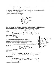
Double integration in polar coordinates. 1. 1. Compute. R f(x, y) dx dy, where f(x,
y) = x2 + y2 and R is the region inside the circle of radius 1, centered at (1,0).
double integral gives us the volume under the surface z = f(x, y), just as a single
... The double integrals in the above examples are the easiest types to evaluate ...
a af. There was no picture or description showing the conventions for measure- ment of the angles or directions. To clar
y z r о x ρ φ z r θ φ. Cartesian. Cylindrical Polar. Spherical Polar. = = = z y x z y x z
φ ρ φ ρ sin cos θ φ θ φ θ cos sin sin cos sin r r r. Unit Vectors. (orthonormal) k e.
Key words: calculus of variations; fractional calculus; multitime Euler–Lagrange
...... [14] R. Hilfer, Applications of fractional calculus in physics, World Sci.
Use MATLAB to plot the boundary of the region in the xy-plane which is
represented in the inte- grals below. Use MATLAB to compute the double integral
.
Multiple Integrals. Double Integrals. Changing to Better Coordinates. Triple
Integrals. Cylindrical and Spherical Coordinates. Vector Calculus. Vector Fields.
Representations of the RGB colour space in terms of 3D-polar coordinates (hue, .... the original colours, and hence that the triangular inequality should be ...
Georges Flandrin2, and Jacques Klossa3. 1. Centre de Morphologie Mathématique, Ecole des Mines de Paris,. 35 rue Saint-Honoré, 77305 Fontainebleau, ...
arXiv:quant-ph/9804037v1 15 Apr 1998. Hamiltonian path integral quantization in polar coordinates. A.K.Kapoor. School of Physics. University of Hyderabad.
cyte , (d) âEchinocyteâ erythrocyte, (e) âBittenâ erythrocyte. 5.1 Algorithm. An algorithm for the extraction of extrusions and the identification of âmush- roomâ class ...
Nov 28, 2012 - Thomas W. Baumgarte,1, 2 Pedro J. Montero,1 Isabel Cordero-Carrión,1 and Ewald Müller1 ...... [19] M. Alcubierre and J. González, Comp.
Sep 24, 2017 - 1. arXiv:1709.08173v1 [math-ph] 24 Sep 2017 ...... (72). âUBV(Ï) = Ï Ï f(-iÏ) = Ï Ï ekÏ the second term follows from f(-iÏ) = ekÏ. We can use ...
We generalize the notions of the fractional q-integral and q-derivative by introducing ... Basic hypergeometric functions, q-integral, q-derivative, fractional calcu- lus. 311 ...... W. A. Al-Salam, A. Verma: A fractional Leibniz q-formula. Pacific .
(a = 0) . 2000 Mathematics Subject Classification. 41A05, 33D60. Key Words and Phrases. Basic hypergeometric functions, q-integral, q-derivative, fractional ...
verting double integrals into iterated integrals in other coordinate systems. .... In
example 2, we used the notation dA to state the problem and dAxy in working.
The geodetic coordinate system and the relationship between spherical and geode- tic coordinates. For brevity we shall often denote the horizontal position in ...
programs represent correctly, in polar coordinates, the relativistic transformation equations for the space-time coordinates of the same event. Special relativity ...
to business: finance, statistics, operations. In finance, for example, ... What follows
is a short, (relatively) non-technical review of those aspects of calculus you'll ...
The Fundamental Theorem of Calculus (F.T.C.) is a general statement about the
relationship ... Reference: S. J. Colley, Vector Calculus, Prentice-Hall, 1999.
Reprinted with permission from Calculus: Early Transcendentals, Third Edition ...
EXAMPLE 5 Prove the formula for the sum of the squares of the first positive.
Vector calculus is the normal language used in applied mathematics for ... In
ordinary differential and integral calculus, you have already seen how derivatives
.
Notes - Double Integrals in Polar Coordinates - Calculus Animations
In the lecture on double integrals over non-rectangular domains we used to ...
However if we reformulate the problem in terms of polar coordinates we have ...
Double Integrals in Polar Coordinates
In the lecture on double integrals over non-rectangular domains we used to demonstrate the basic idea with graphics and animations the following:
However this particular example didn't show up in the examples. The function here is f (xy) over the circle
2
x y
2
=
y
e
9. Had we set up the integral we would have had:
3
3
2
9 x
e
y
dy dx
uh no thanks.
2
9 x
However if we reformulate the problem in terms of polar coordinates we have something much more manageable .
There are 2 issues we must decide 1. How do we set the integration limits ? 2. What form does the areal element dA take--- the answer is not simply drdθ as you might first expect
1. Setting the Integration Limits Typically when polar coordinates are used we have a region such as:
2. The Areal element dA
Recall in Rectangular coordinates we partition the region R according to x = constant- vertical lines and y = constant which are horizontal lines.
This partition creates rectangles with Δ A = Δ xΔ y
which when we let the number of rectangles go to
We obtain dA = dxdy
Suppose we partition the region R according to θ = constant which are lines emanating from the origin and r = constant which are concentric circles centered at the origin.
Recall the length of a circular arc is s = r θ
Speaking without much rigor we have a "rectangle" whose length and width are dr and rdθ and hence dA = rdrdθ . This is a good way of remembering dA but let's be more rigorous.
dA is the difference between the area of the circular sector of radius r and the one of r +dr. Recall the area of a 1 2 circular sector subtended by an angle θ is A r . If we let r denote the midpoint of the segment from r m 2 to r+dr We have :
Therefore in Polar Coordinates The general form of the double Integral is :
=
g ( )
2 f ( ) r d r d g1( )
Example 1 Suppose we have the region inside the Cardioid r 1
Suppose f(x,y) = 2
is the density. Find the Mass. in polar from f(r,θ ) =
x y
2
1 cos( )
3 2
1 r
1 cos () but outside the circle
r dr d
1 r
r
3 2
.
Now α and β are determined from the intersections of the 2 curves
This yields
cos ( )
1
1 r
r dr d
3
3
3
2
2
sin( ) 2
3
2
therefore θ = -π /3 and π /3
1 cos( )
3
3
2
1 cos ( )
3 2
1 cos( )
1 dr d
3 1 cos ( ) d 2
3 2 6 6
3
sin( ) 2
3 3
3
3
.685
3
A couple of questions arise 1. Could we have simply intergrated from 0 to π /3 and double the result ? In general no. Consider the graph at the beginning of this discussion. Even though the areas in the 1st and 4th quadrants are symmetric the surface lying over these regions isn't. We need both symmetry over the region of integration and the surface over that region.
Having said that, in our example f(r,θ ) =1/r is symmetric and so in our example we could have integrated half the region and doubled it.
2. Could we have set the integration limits to be 5π /3 to π /3 ? No if we did we'd be integrating clockwise covering the following region:
Example 2 Evaluate 2 4 y 0
2
1 2
1 x y
dxdy 2
y
Let's consider a graph of the region
4y
x
when
2
is the right half of the circle r = 2 and x = y is the line θ = π /4 . the 2 intersect
4y
2
4y
or
y
2
y
2
or y =
2 . Note since the lower limit on y is 0 we
2
don't need to consider
1
If we convert to polar coordinates
1
2
1 x y
2
1 r
2
2 4 y 0
2
1 2
dxdy
1 x y
2
y
4 2 0
using the u-sub
u
1 r
2
r
r
du
dr
we obtain
2
4 2 0
2
0
1 r
dr d
1 r
r 1 r
dr d 2
4 5 1 du d 0
1
5 1
4
4
5 1
.971
0
Example 3 Suppose we have
Then we are looking at a solid whose height has the constant value 1 therefore the volume is numerically equal to the area of R. i.e. we can use a double integral to compute the area of a plane region.
With this in mind Calculate the Area of the region inside the circle r = 2 and to the right of the line x = 1.
Here we can Compute the Area in the firs quadrant and double the result. What about x = 1 Recall x = r cos(θ )
therefore we have rcos(θ ) = 1 or r = sec(θ )
Therefore r varies from sec(θ ) to 2. What about θ ? At the upper limit sec(θ ) = 2 from which we get θ = π /3
A
3 sec( ) 2 r dr d 0
0
3 2 sec ( ) 2 d 2 0
tan ( )
3
3 0
Example 4
Ok we've been putting it off as long as possible
What about
3
3
2
9 x
e 2
9 x
y
dy dx ?
We can evaluate over the first and fourth quadrant and double the result.
2
3 9 x
3
e 2
9 x
y
dy dx
2 3 r sin( ) e 2 r dr d 0 2
Which brings us to a very important point --- There is no panacea!!!! Even though we now have another tool in or Calculus chest we will always run into problems that can't be solved analytically (you might think integrate by parts--good idea -- try it and get back to me in a year or 2). This is the power of technology -- to get a numerical approximation just highlight the integral and hit equal
2 3 r sin( ) e 2 r d r d 74.519 0 2