Feb 23, 2004 - 2.5 Automorphisms of free groups . ... Warwick Mathematics Institute during the Spring Term of the 1997/98 academic year. This document is the ... It is based heavily on the books of Birman [2] and Hansen [5]. In the first .... from braids with trivial permutation is the pure (or coloured) braid group. 2.2 Artin's ...
Notes on braid groups
Nicholas Jackson February 23, 2004
Contents 1 Braids and Links
1
1.1
Geometric braids . . . . . . . . . . . . . . . . . . . . . . . . . . . . . . . . . . .
1
1.2
Closed braids, links and Markov’s theorem . . . . . . . . . . . . . . . . . . . . .
2
2 Braid groups
4
2.1
Geometric braid groups . . . . . . . . . . . . . . . . . . . . . . . . . . . . . . .
4
2.2
Artin’s presentation . . . . . . . . . . . . . . . . . . . . . . . . . . . . . . . . .
4
2.3
Configuration spaces . . . . . . . . . . . . . . . . . . . . . . . . . . . . . . . . .
6
2.4
Braid groups of manifolds . . . . . . . . . . . . . . . . . . . . . . . . . . . . . .
6
2.4.1
2.5
The braid group of the Euclidean plane E
2
. . . . . . . . . . . . . . . .
7
2.4.2
The braid group of the 2-sphere S . . . . . . . . . . . . . . . . . . . . .
8
2.4.3
The braid group of the projective plane P 2 . . . . . . . . . . . . . . . .
9
Automorphisms of free groups . . . . . . . . . . . . . . . . . . . . . . . . . . . .
10
2
3 Representations of braid groups
12
3.1
Free differential calculus . . . . . . . . . . . . . . . . . . . . . . . . . . . . . . .
12
3.2
Magnus representations . . . . . . . . . . . . . . . . . . . . . . . . . . . . . . .
13
3.3
Burau’s representation of Bn
15
3.4
Gassner’s representation of PB n
. . . . . . . . . . . . . . . . . . . . . . . . . .
15
3.5
Fidelity . . . . . . . . . . . . . . . . . . . . . . . . . . . . . . . . . . . . . . . .
16
. . . . . . . . . . . . . . . . . . . . . . . . . . . .
1
List of Figures 1.1
A geometric n-braid . . . . . . . . . . . . . . . . . . . . . . . . . . . . . . . . .
1
1.2
The closure βb of the braid β, with respect to the axis ` . . . . . . . . . . . . . .
2
1.3
A Markov R-move . . . . . . . . . . . . . . . . . . . . . . . . . . . . . . . . . .
2
1.4
A Markov W-move . . . . . . . . . . . . . . . . . . . . . . . . . . . . . . . . . .
2
1.5
An LU -move on a braid . . . . . . . . . . . . . . . . . . . . . . . . . . . . . . .
3
2.1
Composition of braids . . . . . . . . . . . . . . . . . . . . . . . . . . . . . . . .
4
2.2
The elementary braid σi . . . . . . . . . . . . . . . . . . . . . . . . . . . . . . .
4
2.3
Relations in the elementary braids . . . . . . . . . . . . . . . . . . . . . . . . .
5
2
Abstract This is an expository dissertation on some aspects of the study of braid groups. It is an expanded (and tidier) form of the notes for a graduate seminar I gave at the University of Warwick Mathematics Institute during the Spring Term of the 1997/98 academic year. This document is the ‘director’s cut’, in the sense that it explores the topics in more detail than the original talk, during which there wasn’t enough time to describe the representation theory of the braid groups. It is based heavily on the books of Birman [2] and Hansen [5]. In the first chapter, we consider the geometric properties of braids, and some of their connections to knots and links. The second chapter is concerned with various descriptions of the braid group and some of its generalisations. The third chapter investigates the representation theory of the braid groups.
Chapter 1
Braids and Links In this chapter we investigate some of the geometric properties of braids, looking, in particular, at the connections between braids and links.
1.1
Geometric braids
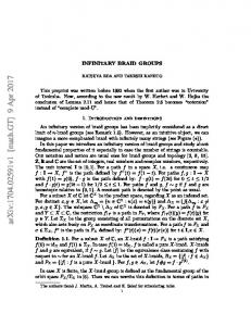
Consider Euclidean 3-space, denoted E 3 , and let E02 and E12 be the two parallel planes with z-coordinates 0 and 1 respectively. Let Pi and Qi (where 1 6 i 6 n) be the points with coordinates (i, 0, 1) and (i, 0, 0) respectively, so that P1 , . . . , Pn lie on the line y = 0 in the upper plane, and Q1 , . . . , Qn lie on the lint y = 0 in the lower plane. A braid on n strings (often called an n-braid) consists of a system of n arcs a1 , . . . , an (the strings of the braid), such that ai connects the point Pi in the upper plane to the point Qπ(i) in the lower plane, for some permutation π ∈ Symn . Furthermore: (i) Each arc ai intersects the plane z = t once and once only, for any t ∈ [0, 1]. (ii) The arcs a1 , . . . , an intersect the plane z = t in n distinct points for all t ∈ [0, 1]. In other words, an n-braid β consists of n strands which cross each other a finite number of times, do not intersect with themselves or any of the other strands, and travel strictly downwards, as depicted in figure 1.1. q q q · · P·n−q 1 Pqn
P1 P 2 P3
··· q q q · · Q· q Qq
Q1 Q2 Q3
n−1
n
Figure 1.1: A geometric n-braid The permutation π is called the permutation of the braid. If this permutation is trivial then β is said to be a pure (or coloured) braid. 1
Two braids β0 and β1 with the same permutation π are said to be equivalent or homotopic if there is a homotopy through braids βt each with permutation π, where t ∈ [0, 1], from β0 to β1 . Alternatively, β0 and β1 are equivalent if there exists an ambient isotopy of E 3 from β0 to β1 which fixes E02 and E12 .
1.2
Closed braids, links and Markov’s theorem
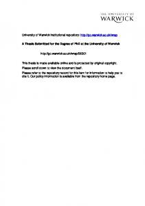
It transpires that there is a fundamental connection between braids and links. Define the closure βb of a braid β by identifying each of the points Pi in the plane E12 with the corresponding point Qi in E02 — this is equivalent to joining the points Pi and Qi by a series of concentric arcs as shown in figure 1.2. The closed braid βb is then said to be closed with respect to the axis `.
β
q `
Figure 1.2: The closure βb of the braid β, with respect to the axis ` Theorem 1.1 (Alexander 1923) Every link is isotopic to a closed braid. A stronger version of this result is due to Markov, and shows how two closed braid representatives of a given link are related to one another. Let moves of type R and W be, as indicated in figures 1.2 and 1.2, the replacement of a segment of a closed braid βb by (respectively) two or three edges. q`
� � � �
q`
6
�-
� �
-
Figure 1.3: A Markov R-move `q �
�-
6 `q -
Figure 1.4: A Markov W-move Theorem 1.2 (Markov 1935) If α b and γ b are two isotopic closed braids, then there exists a finite sequence of closed braids c0 , . . . , βbs = γ α b=β b 2
such that each βbi differs from βd i−1 by a single move of type R or type W or their inverses. A proof of this is due to Birman [2]. A refinement of this result — a one-move version of Markov’s theorem — was proved in 1997 by Rourke and Lambropoulou [7]. This theorem makes use of an operation called an L-move, depicted in figure 1.2, where a string is cut and two more vertical strands are attached to the ends, passing either over or under all the other strands of the braid. There are thus two different types of L-move, LO and LU , but these are essentially the same operation.
@
@ @ @
�-
@ @
�-
@ @ @
Figure 1.5: An LU -move on a braid
3
Chapter 2
Braid groups 2.1
Geometric braid groups
Given two n-braids, α and β, there is an obvious way of combining them to form a third n-braid αβ: attach β to the end of α as depicted in figure 2.1. This operation is called composition, and defines a group structure on the set of n-braids. The identity element is the braid formed from n parallel strands with no crossings, and the inverse β −1 of a braid β is formed by reflecting β in a horizontal plane. α αβ
β
Figure 2.1: Composition of braids This group, the n-string braid group is denoted by Bn . The subgroup PB n of Bn formed from braids with trivial permutation is the pure (or coloured) braid group.
2.2
Artin’s presentation
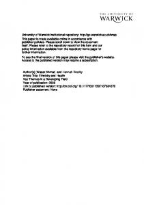
Notice that any n-braid can be formed by a finite number of elementary braids σ1 , . . . , σn−1 , where σi corresponds to the geometric n-braid formed by crossing the ith string over the (i+1)th string, as depicted in figure 2.2. i i+1
···
···
Figure 2.2: The elementary braid σi We then notice that if i and j differ by more than one, then the elementary braids σi and σj 4
commute. Furthermore, there is an analogue for braids of the third Reidemeister move for knots and links which, written in terms of the elementary braids, becomes σi σi+1 σi = σi+1 σi σi+1 . i i+1 i+2
i i+1 i+2 i i+1
i i+1
j j+1
j j+1
σi
σi+1
σi
σj
σi
�-
�- σi+1
σj
σi
σi
σi+1 σi σj = σj σi
σi+1 σi σi+1 = σi σi+1 σi
Figure 2.3: Relations in the elementary braids The following theorem, due to Emil Artin, says that these two relations are sufficient to describe the n-string braid group: Theorem 2.1 (Artin) Bn ∼ = hσ1 , . . . , σn−1 |σi σj = σj σi if |i − j| > 1, σi σi+1 σi = σi+1 σi σi+1 i In other words, the n-string braid group is generated by generators σ1 , . . . , σn−1 subject to relations (i) σi σj = σj σi if |i − j| > 1. (ii) σi σi+1 σi = σi+1 σi σi+1 for 1 6 i 6 n − 2. The pure braid group, PBn , can be considered as the subgroup of Bn consisting of braids which induce the identity permutation: Theorem 2.2 The pure braid group PBn has a presentation with generators: −1 −1 −1 Aij = σj−1 σj−2 . . . σi+1 σi2 σi+1 . . . σj−2 σj−1
where 1 6 i < j 6 n, and relations:
Ars Aij A−1 rs
Aij A−1 A A ij is is = −1 −1 A A ir Aij Air Aij ij −1 −1 −1 A−1 A is ir Ais Air Aij Air Ais Air Ais
s < i or j < r i 2 and M is neither P 2 nor S 2 , then 0
−→
2.4.2
π1 (Fn−1,1 (M )) k An (M )
−→
π1 (Fn (M )) k PBn (M )
−→
π1 (Fn−1 (M )) k PBn−1 (M )
−→
0
The braid group of the 2-sphere S 2
The braid group of the 2-sphere is similar to the braid group of the Euclidean plane, except that the points move on S 2 instead. An S 2 -braid may be depicted geometrically as a braid between two concentric spheres. The group Bn (S 2 ) is generated by the same generators σi and relations as Bn (E 2 ), but with one additional relation: (iii) σ1 σ2 . . . σn−1 σn−1 . . . σ2 σ1 = 1 This requirement says, geometrically, that the braid formed by taking the first string round behind all of the other strings and back in front of them, back to its starting position, is equivalent to the trivial braid. By considering the geometric depiction of an S 2 -braid described above, we see that this is true, since the loop may be pushed off the inner sphere without tangling with any of the other strings. As before, we can construct a fundamental exact sequence for Bn (S 2 ): j
i
0 −→ An (S 2 ) −→ PBn (S 2 ) −→ PBn−1 (S 2 ) −→ 0
8
The remark at the end of the previous subsection suggests that the braid groups of the 2-sphere and the projective plane might have some strange properties not shared by the braid groups of arbitrary 2-manifolds. This is further suggested by the following: Theorem 2.7 (Newwirth) If M is either E 2 or any compact 2-manifold except P 2 or S 2 then neither Bn (M ) nor PB n (M ) have any nontrivial elements of finite order. So, is Bn (S n ) torsion-free? Or can we find a nontrivial element of finite order? Theorem 2.8 (Fadell/Newwirth 1962) The word σ1 σ2 . . . σn−1 has order 2n in Bn (S 2 ). This can be seen geometrically, with a little imagination. The word σ1 σ2 . . . σn−1 corresponds to taking the first string over all the others to the nth position. If we do this n times, then each of the strings ends up back where it started, making a pure braid. If we then do the same thing a further n times (making 2n in total), each string winds round the remaining n − 1 strings twice. We may then utilise a move known as the ‘Dirac string trick’ (qv [5] for a series of diagrams depicting this operation) to untangle all n strings, resulting in a trivial braid. What are some of these groups Bn (S 2 ) like? Notice that Bn (E 2 ) is infinite for n > 1, but the previous theorem suggests that this might not necessarily be the case for the braid groups of the 2-sphere. In fact: PB2 (S 2 ) B2 (S 2 ) PB3 (S 2 ) B3 (S 2 )
2.4.3
=0 = Z2 = Z2 is a ZS-metacyclic group of order 12
The braid group of the projective plane P 2
We now consider the braid group of the projective plane. Recall that P 2 is the 2-disc D2 with antipodal boundary points identified. It is not embeddable in R3 and is hence not particularly easy to visualise. The group Bn (P 2 ) is generated by σ1 , . . . , σn−1 (as for the braid groups of the plane and the 2-sphere), and ρ1 , . . . , ρn , subject to the same relations as for Bn (E 2 ), with the following additional relations: (iii) σi ρj = ρj σi if |i − j| > 1 (iv) ρi = σi ρi+1 σi −1 2 (v) ρ−1 i+1 ρi ρi+1 ρi = σi
(vi) ρ21 = σ1 σ2 . . . σn−1 σn−1 . . . σ2 σ1 These generators each have a geometric interpretation — the σi may be regarded as the ith string passing in front of the (i + 1)th string, and ρi may be depicted as the ith string moving
9
forwards towards the boundary of D2 and then reappearing at the corresponding antipodal point before returning to its starting position. As before, we get a fundamental exact sequence: j
i
0 −→ An (P 2 ) −→ PBn (P 2 ) −→ PBn−1 (P 2 ) −→ 0 It transpires, also, that Bn (P 2 ) has a torsion element: Theorem 2.9 (van Buskirk 1966) The word σ1 . . . σn−1 has order 2n in Bn (P 2 ) In addition, there are nontrivial braid groups of finite order, as with the S 2 case: B1 (P 2 ) B2 (P 2 ) PB2 (P 2 ) A2 (P 2 ) Bn (P 2 )
2.5
= Z2 is dicyclic of order 16 is the quaternion group = Z4 is infinite for n > 3
Automorphisms of free groups
There is an alternative definition of the braid groups in terms of subgroups of Aut Fn , the group of (right) automorphisms of the free group of rank n. Theorem 2.10 (Artin Representation Theorem) Let Fn be the free group on n generators: hx1 , . . . , xn |i. Then Bn is isomorphic to the subgroup of Aut Fn consisting of all right automorphisms β on Fn such that xi β = Ai xτ (i) A−1 i (x1 . . . xn )β = x1 . . . xn where 1 6 i 6 n, τ ∈ Symn , and Ai is some word in Fn . Under this isomorphism, σi corresponds to an automorphism σi of Fn , where xi σi = xi xi+1 x−1 i xi+1 σi = xi xj σi = xj for all j 6= i, i + 1. The permutation τ for the automorphism β is the permutation of the braid β. Justification Identify Fn with the fundamental group of the n-punctured plane: Fn ∼ = π1 (E12 \ {P1 , . . . , Pn }, P0 ) ∼ = π1 (E02 \ {Q1 , . . . , Qn }, Q0 ) 10
where P0 = (0, 0, 1) and Q0 = (0, 0, 0). Thus, each generator xi ∈ Fn corresponds to a loop, based at P0 , passing anticlockwise round Pi . Now consider a geometric braid β ∈ Bn in terms of the slab of E 3 between E02 and E12 with the strings of the braid removed. Then a braid β lifts to a map β : Fn = π1 (E12 \ {P1 , . . . , Pn }, P0 ) → Fn = π1 (E02 \ {Q1 , . . . , Qn }, Q0 ). Geometrically, we visualise this by constructing the loop ` round the Pi corresponding to the word in Fn , and then push ` down the braid. Note that this is a single-valued mapping on homotopy classes and a homomorphism. Furthermore, it is a right automorphism — the inverse may be constructed by pushing the loop back up the braid again. The homotopy of braids says that if β1 and β2 are homotopic then β1 = β2 . The mapping Bn → Aut Fn given by β 7→ β is a homomorphism, since β1 β2 = β1 β2 . Given that the word x1 . . . xn corresponds to an anticlockwise loop round all the Pi , it will be unchanged by the automorphism given by any n-braid β: (x1 . . . xn )β = x1 . . . xn . Considering the action of the automorphisms σi (where σi is the ith elementary braid), we see that: xi+1 σi = xi xi σi = xi xi+1 x−1 i xj σi = xj 2
if j 6= i, i + 1.
11
Chapter 3
Representations of braid groups In this chapter we provide a brief overview of Fox’ free differential calculus, show how it may be used to construct matrix representations of automorphism groups of Fn , and then look at two examples, namely Burau and Gassner’s representations of, respectively, Bn and PBn .
3.1
Free differential calculus
Let Fn be a free group of rank n, with basis {x1 , . . . , xn }, and let φ be a homomorphism acting on Fn , with Fnφ denoting the image of Fn under φ. P Now let ZFnφ denote the integral group ring of Fnφ : an element of ZFnφ is a sum ag g, where ag ∈ Z and g ∈ Fnφ , with addition and multiplication defined by
�X
X
ag g +
X
ag g
� �X
Bg g =
X
(ag + Bg )g !
�
Bg g =
X X g
agh−1 Bh
g
h
A homomorphism ψ : Fnφ → Fnψφ induces a ring homomorphism ψ : ZFnφ → ZFnψφ . Later we will consider the cases where ψ is the abelianiser a or the trivialiser t. There is a well-defined mapping ∂ : ZFn → ZFn ∂xj given by r
1 � X ∂ (ε −1) xεµ11 . . . xεµrr = εi δµi ,j xεµ11 . . . xµ2i i ∂xj i=1
� X ∂ �X ∂g ag g = ag ∂xj ∂xj where g ∈ Fn , ag ∈ Z, εi = ±1, and δµi ,j is the Kronecker δ. The following properties follow from the definition: 12
Proposition 3.1 ∂xi (i) ∂x = δi,j . j ∂x−1 i ∂xj
= −δi,j x−1 i . � � � � ∂w ∂v τ (iii) ∂(wv) = v + w ∂xj ∂xj ∂xj . (ii)
3.2
Magnus representations
Let Sn be a free abelian semigroup with basis {s1 , . . . , sn }, let R be a ring, and let A0 (R, Sn ) be the semigroup ring of Sn with respect to R: elements in A0 (R, Sn ) are polynomials in non-negative powers of the si (which all commute), with coefficients in R. Now define τ : Fn → M2 A0 (ZFn , Sn ) as: � w 7→ [w] =
Pn
∂w j=1 ∂xj sj
w 0
�
1
In particular: � xj 7→ [xi ] = (Since
Pn
∂xi j=1 ∂xj sj
=
Pn
j=1 δij sj
xi 0
si 1
�
= si .)
If w, v ∈ Fn then [wv] = [w][v]. The mapping w 7→ [w] is a representation, the Magnus representation, of Fn , and is not particularly interesting. If, though, we have a homomorphism φ acting on Fn , and let " φ
w 7→ [w] =
wφ 0
Pn
j=1
�
∂w ∂xj
�φ
sj
#
1
then this is also a representation, the Magnus φ-representation of Fn : [Fn ]φ is the image of Fn under this homomorphism Φ : Fn → [Fn ]φ ; w 7→ [w]φ . We can generalise this representation Φ to representations of Fn by k × k upper-triangular matrices: Define higher-order derivatives inductively (writing Dj for
Di1 i2 ...iq (w) D(w)
= Diq (Di1 i2 ...iq−1 (w)) n X = Di (w)si i=1
D
q+1
(w)
∂ ∂xj ).
= D(Dq (w))
Then: 13
Dq+1 (w)
X
=
Di1 ...iq (w)si1 . . . siq
16ij 6n
Dq (uv)
=
q−1 X
(Dp (u)(Dq−p (v))t + uDq (v)
p=1
where t is the trivialiser. Theorem 3.2 (Enright 1968) Let φ be a homomorphism of Fn and let (Dq (w))φ be the image of Dq (w) under the ring homomorphism induced by φ. Then, for w ∈ Fn , let {w} = φ
wφ 0 0 .. .
(D(w))φ 1 0 .. .
(D2 (w))φ (D(w))t 1 .. .
(D3 (w))φ (D2 (w))t (D(w))t .. .
··· ··· ···
(Dk−1 (w))φ (Dk−2 (w))t (Dk−3 (w))t .. .
0
0
0
0
···
1
Then Φ : w 7→ {w}φ defines a representation of Fn in the ring Mk (A0 (ZFn , Sn )) of k × k matrices over A0 (ZFn , Sn ) for k > 2 and φ a homomorphism acting on Fn . Corollary 3.3 Let xi be a basis element of Fn . Then: t xi → 7 {xi } =
1
si
0
0 1 .. . . . . .. . 0 ···
si 1 .. . ···
··· .. . .. . .. . 0
0 .. . 0 si 1
is a faithful matrix representation of Fn modulo the kth group of the lower central series of Fn over A0 (ZFn , Sn ) for k > 2. The point of all this is that we can now use this machinery of Magnus representations to study subgroups of Aut Fn , such as Bn or PBn . Let φ be a homomorphism acting on Fn and let Aφ be any group of (right) automorphisms of Fn which satisfy xφ = xαφ for all x ∈ Fn and α ∈ Aφ . So, if φ is the abelianiser a, then Aφ might be the subgroup of Aut Fn mapping each element into a conjugate of itself. Any subgroup of Aut Fn inducing the identity automorphism on Fn /Fn0 could do. 14
Now, if α ∈ Aφ , define τ : α 7→ kαkφ =
��
∂(xi α) ∂xj
�φ � . Thus, τ defines a representation
Aφ → Mn (ZFnφ ). For example: Example 3.1 Let φ be t, the trivialiser t : Fn → 1, and At be Aut Fn . Then t maps each element of Aut Fn to an n × n matrix over Z where the (i, j)th element is the exponent sum of xj in wi . These matrices are invertible, and so have determinant ±1, hence Fnt is a subgroup of the unimodular group.
3.3
Burau’s representation of Bn
As noted before, Bn has a faithful representation as a group of automorphisms of Fn , and hence we can regard Bn as a subgroup of Aut Fn . Let Z = hti be the infinite cyclic group, and let ψ : Fn → Z; xi 7→ t. Then the corresponding representation, the Burau representation of Bn is given by:
Ii−1 0 ψ σi → 7 kσi k = 0 0
3.4
0 1−t 1 0
0 0 t 0 0 0 0 In−i−1
Gassner’s representation of PB n
To represent the pure braid groups PBn , we can simply restrict the Burau representation of Bn . But a more interesting representation exists, discovered by B.J. Gassner in 1961[4]: Let φ be the abelianiser a. Then PBn has a representation as a subgroup of Aut Fn by the restriction of ξ : Bn → Aut Fn to PBn . Let AF n be the free abelian group of rank n, with basis {t1 , . . . , tn } and let a : Fn → AF n be defined by xi a = ti . The pure braid generators map a generator xi of Fn into a conjugate of itself, so the requirement xi Ars a = xi a is satisfied for 1 6 i 6 n and 1 6 r < s 6 n if φ = a. So, we derive the Gassner representation of PBn : δij (1 − ti )δir + tr δij a ((Ars ))ij = (1 − ti )(δij + ti δsj ) + ti ts δij (1 − ti )(1 − ts )δrj − (1 − tr )δsj + δij
15
if if if if
s < i or i < r s=i r=i r 6. The question regarding the Burau representation of B4 and B5 has not as yet been settled.
16
Bibliography [1] Joan Birman. On braid groups. Communications on Pure and Applied Mathematics, 22:41–72, 1969. [2] Joan Birman. Braids, Links, and Mapping Class Groups, volume 82 of Annals of Mathematics Studies. Princeton University Press, 1974. [3] Edward Fadell and L. Neuwirth. Configuration spaces. Mathematica Scandinavica, 10:111–118, 1962. [4] Betty Jane Gassner. On braid groups. Abhandlungen aus dem Mathematischen Seminar der Universit¨ at Hamburg, 25:10–22, 1961. [5] Vagn Lundsgaard Hansen. Braids and Coverings: Selected Topics, volume 18 of London Mathematical Society Student Texts. Cambridge University Press, 1989. [6] John Moody. The faithfulness question for the Burau representation. Proceedings of the American Mathematical Society, 119(2):671–679, 1993. [7] Colin Rourke and Sofia Lambropoulou. Markov’s theorem in 3-manifolds. Topology and its Applications, 78:95–122, 1997.
17