Mar 12, 2012 - Martin Eichenbaum. March 12 ...... Panel B: Increase in Ï from 0.775 to 0.793 (longer expected duration of lower bound). dGDP. dG. &2.84. 5.36.
Notes on Linear Approximations, Equilibrium Multiplicity and E-learnability in the Analysis of the Zero Lower Bound Lawrence J. Christiano
Martin Eichenbaum
March 12, 2012
We are very grateful for discussions with Anton Braun, Luca Dedola, Giorgio Primiceri, and Mirko Wiederholt. We are particularly grateful to Marco Bassetto for encouraging us to consider E-learnability.
Abstract We study the properties of the zero lower bound model in Eggertson and Woodford (2003) (EW). EW’s analysis is based on the equilibrium conditions after linearization. Working with the actual nonlinear equilibrium conditions and consistent with Braun, Körber and Waki (2012) and Mertens and Ravn (2011), we …nd the existence of equilibria that are not visible to analyses based on linearization, as well as sunspot equilibria. These …ndings challenge the …ndings about the properties of the zlb reported in Christiano, Eichenbaum and Rebelo (2011), Eggertson (2011), EW and others. However, we …nd that the equilibria that are ‘invisible’to analyses using linearization are not E-learnable and so those equilibria may perhaps be treated as mathematical curiosities. In addition, evidence that the quality of linear approximations is poor rests on examples where output deviates by more than 20 percent from its steady state, cases where no one would expect linear approximations to work well. For perturbations of reasonable size, the conclusions arrived at in the zlb analysis that use linear approximations appear to be robust.
1. Introduction In an in‡uential paper, Eggertsson and Woodford (2003) (EW) studied an equilibrium for a simple New Keynesian model without capital in which the zero lower bound on the nominal rate of interest (zlb) is binding. A well-chosen set of simplifying assumptions on the environment greatly simpli…ed the analysis. EW studied an equilibrium which is characterized by two numbers, in‡ation and output when the zlb binds, and two equations. In the equilibria they study, the system jumps immediately to steady state as soon as the shock that makes the zlb bind goes away. 2
Because the equations are linearized, there is a unique solution. The analysis is so in‡uential in part because its simplicity permits a straightforward analytic derivation of a number of interesting results. These results include (see, for example, EW, Eggertsson (2011) and Christiano, Eichenbaum and Rebelo (2011) (CER)): When the zlb binds, the loss in output is potentially substantial. The output multiplier on government consumption is larger when the zlb binds than when it does not bind. When prices are more ‡exible, or the expected duration of the zlb is longer, then the magnitude in the drop in output in the zlb is greater and the government consumption multiplier is larger. In this paper, we restrict ourselves to the type of equilibria considered in EW. That is, we consider equilibria in which the system jumps to a particular steady state as soon as the shock is over. In addition, equilibrium while the zlb binds is characterized by constant numbers. We depart from EW by not linearizing the equilibrium conditions. We do this using the strategy followed in Braun, Körber and Waki (2012), who interpret the price frictions in the EW analysis as stemming from adjustment costs as proposed by Rotemberg (1982). This interpretation is interesting because it implies the same linearized equations that EW study. An alternative approach which also implies the linearized equations studied by EW is based on the price setting frictions proposed by Calvo. The advantage of adopting Rotemberg adjustment costs here is analytic simplicity. The Calvo approach injects an endogenous state variable (past price dispersion), while there is no endogenous state variable in the Rotemberg approach. 3
We …nd that the key qualitative results listed above survive our nonlinear analysis. Our argument takes the following form. First, as in Braun, Körber and Waki (2012) we …nd that there are multiple equilibria, including the sunspot equilibrium documented in Mertens and Ravn (2011). If we look across all the equilibria, one can argue that the conclusions described in the bullets above are not robust.1 For example, in the sunspot equilibrium the government consumption multiplier is smaller when the zlb binds than when it does not bind. This ‡atly contradicts a key claim in the literature. Second, we impose the requirement that equilibria be E-learnable. Subject to this re…nement the model has a unique equilibrium. Third, the properties of the unique equilibrium have the properties stressed in the existing zlb literature. A caveat to our results is that E-learnability requires taking a stand on a learning mechanism. We are currently exploring alternative learning mechanisms and re…nement criteria. Section 2 below describes our model. Section 3 discusses model steady states and relates our analysis to that of Benhabib, Schmitt-Grohe and Uribe (2001). Section 4 de…nes the set of equilibria that we study. Section 5 derives the linearized equilibrium conditions of the model. This establishes a baseline for comparison. Section 6 discusses E-learnability and describes the learning rule that we employ. Section 7 presents our results for EW equilibria. Finally, section 8 reviews the sort of calculations that are done when researchers wish to go beyond qualitative results used to develop intuition about the properties of economies in the zlb. In practice, those researchers often apply deterministic simulation methods. We investigate the quality of the of the linear approximations within that context. Conclusions appear in section 9. 1
It is not even clear how one de…nes a multiplier when there are multiple equilibria. Before and
after the jump in G there are two sets of equilibria.
4
2. Model A representative household maximizes E0
1 X t=0
t
h
log (Ct )
2
h2t
i
subject to Pt Ct + Bt where
t
(1 + Rt 1 ) Bt
1
+ Wt ht +
t;
represents lump-sum pro…ts net of lump-sum government taxes. The …rst
order necessary conditions associated with an interior optimum are: ht Ct =
Wt 1 Pt Ct ; = Et : Pt 1 + R t Pt+1 Ct+1
Aggregate output, Yt ; is produced by representative, competitive …nal good producer using intermediate goods, Yjt ; j 2 [0; 1] : The production function and …rst order conditions are: Z
Yt =
1
" 1 "
" " 1
Yj;t dj
; "
0
1; Yj;t =
Pj;t Pt
"
Yt :
Each intermediate good is produced by a monopolist. The monopolist that produces the j th good has the following objective: Et
1 X
labor costs of production l
t+l [(1
z }| { st+l Pt+l Yj;t+l
+ ) Pj;t+l Yj;t+l
l=0
cost (in terms of …nal goods) of adjusting prices related to aggregate level of output
z
2
where
t
Pj;t+l Pj;t+l 1
}|
2
1
{
(Ct+l + Gt+l )
Pt+l ];
denotes the state and date-contingent value assigned to payments sent to
households. When
= 1; then adjustment costs in changing prices are related to
aggregate GDP, Ct + Gt ; and when
= 0 they are related to the level of household 5
consumption only. We also allow for intermediate cases, because it is not clear on a priori grounds which speci…cation is more sensible. Finally,
is a subsidy to …rms
to address distortions due to monopoly power. We assume 1+
=
" "
1
:
The j th intermediate good producer takes the …rst order condition of the representative …nal good producer as its demand curve. The production function and level of …rm marginal cost (excluding costs associated with price changes) are given by: real marginal cost
z}|{ Wt Pt
production function
Yj;t =
z}|{ hj;t
; st
household optimization
z }| { ht Ct
=
The …rm is required to satisfy whatever demand occurs at its posted price, so that we can substitute out for Yjt using the …rm’s demand curve. Doing this and imposing t
= 1=(Pt Ct ): max1 Et fPj;l gl=0 Pt+l st+l
1 X l=0
l
1 [(1 + ) Pj;t+l Pt+l Ct+l
Pj;t+l Pt+l
"
Yt+l
Pj;t+l Pj;t+l 1
2
Pj;t+l Pt+l
"
Yt+l
2
1
Pt+l (Ct+l + Gt+l )]:
The …rst order condition is, after rearranging: Pj;t " = st + Pt " 1 " Pj;t Ct 1 Pj;t Pj;t (Ct + Gt ) [ 1 " 1 Pt Yt Pj;t 1 Pj;t 1 Ct Pj;t+1 Pj;t+1 Ct+1 + Gt+1 1 ] + Et Pj;t Pj;t Ct+1 (1 + )
When
= 0; the j th …rm simply sets price, Pj;t ; to a markup, "= ("
(2.1)
1) ; over
marginal cost. If that price is high relative to yesterday’s price, then the …rm raises 6
Pj;t by less if
> 0; according to the …rst term in square brackets. Similarly, the
second expression in square brackets implies that if that price is low relative to next period’s price, then the …rm raises price by more if
> 0: Impose the equilibrium
condition, Pj;t = Pi;t = Pt for all i; j; and rearrange: (
t
1)
t
=
1
"
1+
+ Et (
t+1
(1
"
1
1)
t+1
") + " (st
1)
Yt Ct + Gt
(Ct+1 + Gt+1 ) Ct : Ct+1 Ct + Gt
We adopt the assumption that a su¢ cient subsidy is provided to intermediate goods producers so that, at least in steady state, the monopoly distortion is eliminated: "
1+
"
1
:
There are three uses of gross …nal output: household and government consumption, and goods used up in changing prices: Ct + Gt +
2
(
t
1)2 (Ct + Gt )
Yt :
In equilibrium, this is satis…ed as an equality because households and government go to the boundary of their budget constraints. Government consumption is an exogenous process discussed below. The four equilibrium conditions associated with the four unknowns, are:
7
t ; Ct ; Rt ; ht ;
(
t
1 Ct 1 = Et Rt 1 + rt t+1 Ct+1 1 Yt 1) t = " (st 1) Ct + Gt 1 + Et ( t+1 1) 1 + rt Ct + Gt + Rt = max 1;
1
2
(
+
(2.3) t+1
(Ct+1 + Gt+1 ) Ct Ct+1 Ct + Gt
1)2 (Ct + Gt ) = ht
t
(
(2.2)
t
1) :
(2.4) (2.5) (2.6)
The last equation is the monetary policy rule. We suppose that rt 2 rl ; rh . The economy starts with rt = rl in the initial period; and it jumps to rh (
1=
1) with constant probability 1
p: With prob-
ability p; the discount rate remains at its initial, low, value. The higher level, rh ; is an absorbing state for rt . There are no other stochastic shocks in the system. We consider two types of equilibria. In one, rl < 0 and rh > 0: We call this a ‘fundamental equilibrium’, because the shock a¤ects preferences. We also consider a sunspot equilibrium, in which rl = rh ; so that the uncertainty does not a¤ect preferences or technology.
3. Model Steady States Given our assumption about the exogenous shock process, the exogenous randomness settles down eventually in its absorbing state. As a result, the model has a well de…ned steady state. Benhabib, Schmitt-Grohe and Uribe (2001) drew attention to the fact that a model economy like ours has two steady states. They created a diagram, Figure 1, that makes this particularly clear. Two of the equilibrium conditions of the model include the monetary policy rule and the steady state version 8
of the intertemporal Euler equation: R = max 1; R =
1
+
(
1)
= ;
respectively. Figure 1 shows that the above two equations have two crossings. The two steady states involve
= 1 and
= : Once the in‡ation rate is selected, then
the Phillips curve and aggregate output relations can be used to determine steady state C and h : (
1)
=
1
" ( Ch
C +G+
1) 2
(
h + ( C+ G
1)
1)2 (C + G) = h:
Our baseline parameters are: G = 0:20; When steady state is
= 0:99; "= = 0:03;
= 100;
= 1:25;
= 0:
= ; then C = 0:7971 and h = 1:001: When the steady state
= 1; then C = 0:80 and h = 1: The di¤erence is quite small. From here
on, we follow EW in assuming that when the shock switches to its high value, the economy jumps to the higher of the two steady states. One rationale for selecting this steady state may be that the monetary policy rule is actually composed of the Taylor rule with an escape clause which speci…es that if in‡ation is not proceeding at its target rate (i.e., in‡ation is negative versus its target value of zero) then the money growth rate is adjusted. Fleshing out this argument, of course, must be done by introducing money demand and supply. However, with enough separability, this can be done without changing the equilibrium conditions that we work with here (see, for example, Christiano and Rostagno (2001)). 9
4. An Interior, EW Equilibrium An interior EW equilibrium is a set of eight numbers: h
; C h ; Rh ; hh ;
l
; C l ; Rl ; hl ;
that satisfy the equilibrium conditions for the two values of the exogenous shock, ‘h’ for when rt = rh and ‘l’for when rt = rl . In the low state:
1 1 Cl = p + (1 lC l Rl 1 + rl l
l
1
=
1 +
"
l
hC
l
C l + Gl + Rl = max 1;
1
C l + Gl +
1
1 p 1 + rl
l
l
1 l
1
2 +
Cl hC h
p)
l
2
l
2
1 C l + Gl C l + Gl
+ (1
2
(4.1)
h
p)
1
h
1+
(4.2) g
1
C l + Gl = hl .
1
g
Cl C l + Gl (4.3) (4.4)
Following the discussion in section 3, we suppose that the high state is the steady state. We assume that government consumption in that state satis…es: Gh = where
g
C h + Gh ;
g
is the share of government consumption in GDP. Thus, Gh =
g
1
C h: g
In addition, it is easy to con…rm that the other variables take on the following values in the high state: h
= 1;
hh C h = 1; C h = 1 10
g
hh ; Rh = 1 + rh = 1= :
Also, hh =
C
h
"
=
1
1 1
g
g
"
#1=2 1 1
g
#1=2
:
These levels of employment and consumption are the ‘…rst-best’allocations, i.e., the allocations a planner would choose, who is constrained only by the preferences and technology and who ignores prices and price adjustment costs. Conditional on the high-state equilibrium, we can solve for C l ;
l
; hl using the
three low-state equilibrium conditions, (4.1)-(4.4). The algorithm …xes
l
and com-
putes C l and hl using (4.1), (4.3) and (4.4). We then evaluate whether (4.2) holds. If we can …nd a value for …nd such a value of
l
l
such that it holds, we have an equilibrium. If we cannot
; we say there does not exist an interior EW equilibrium. We
use the adjective, ‘interior’ here, to emphasize that we only consider equilibria in which the …rst order conditions of the agents hold with equality. The task of …nding an equilibrium or asserting with con…dence that one does not exist is greatly simpli…ed by the fact that non-negativity of the C l and hl that solve (4.1), (4.3) and (4.4) for given
l
requires that
l
lie in the interior of a particular
bounded and convex set, D. We call the set of in‡ation rates, D; the ‘set of candidate equilibrium in‡ation rates’. We now construct this set. The monetary policy rule divides the candidate in‡ation rates into a subinterval in which the zlb is binding and a second one in which it is not: 8 l l < 1+ 1 ub Rl = ; lub = : 1+ l l 1 > lub 11
1
:
(4.5)
l
Solving the intertemporal Euler condition for Cl after imposing Rl = l
h
l
=
l ub
and using (4.5), we obtain:
1 + rl p 1l h C ; 1 p
(4.6)
= 1: All objects on the right of (4.6) are known, except for
: Thus, this equation provides a mapping from
l
to C l : The fact that we only
consider interior equilibria (i.e., those with hl ; C l > 0) implies a lower bound, l
l lb ;
on
: l lb
p : 1 + rl
=
The function, C l ( l ) in (4.6) is zero at positive, for Cl
l
l lb
0. If gross in‡ation were not positive, sign restrictions on the price level
and consumption (see (8.1)) would be violated: That each backward simulation step requires …nding the zero of a nonlinear function draws attention to two possibilities: (i) there may be no
t
> 0 that solves the nonlinear equation for some t, in which
case there is no interior (i.e., where the e¢ ciency conditions hold with equality) equilibrium and (ii) there may be multiple values of
t
> 0 that solve the nonlinear
equation. To ensure that we do not miss (ii), we initiate the zero-…nding for each t 10
When there is a given initial state, then this backward solution strategy requires back-
ward ‘shooting’, as in Christiano, Braggion and Roldos (2009). To see how this backward approach works in a stochastic setting when the equilibrium conditions have been linearized, see http://faculty.wcas.northwestern.edu/~lchrist/course/Korea_2012/…xing_interest_rate.pdf
36
by …rst placing a …ne grid on a range of values of
t
that extends from nearly zero
to 1.02. As before, we solve the model twice. The …rst time, we solve it for the case where Gt is unchanged relative to its value in steady state. In the other case, Gt is increased by 5 percent in each of periods t = 1; :::; T
1: This second computation
allows us to deduce the government spending multiplier. We now turn to the solution of the log-linearized system, (5.1)-(5.3). It is convenient to express the Phillips curve in terms of y^t ; as in (5.4) (except, here p = 1): y^t =
1 2
g
1
^t
g
^ t+1 +
1
g
^t : G
(8.4)
g
Conditional on ^ t+1 ; this represents a linear restriction across y^t and ^ t : The IS curve and policy rule (i.e., (5.1) and (5.3)) are: y^t
^
g Gt
= y^t+1
^
g Gt+1
Rt = max 1;
1
+
(
1
g
[ (Rt
t
1) ;
1
rt )
^ t+1 ]
(8.5) (8.6)
respectively. We solve (8.4)-(8.6) by applying the same backward simulation strategy just described for (8.1)-(8.3). The calculations are initiated by setting ^ T = y^T = 0: At the tth step, we take ^ t+1 and y^t+1 as given and compute ^ t and y^t that solve (8.4)-(8.6). We convert the problem of solving (8.4)-(8.6) into that of solving one (nonlinear, because of (8.6)) equation in one unknown, ^ t : Given ^ t we use (8.4) to solve for y^t and (8.6) to solve for Rt : Finally, we adjust ^ t until (8.5) is satis…ed, if this is possible. We compute the government consumption multiplier at each date by (~ yt where yt denotes GDP (
Ct + Gt ) and a tilde over a variable indicates 8 < 1:05 Gh t = 1; :::; T 1 Gt = ; : Gh t=T 37
~t yt ) = G
Gt ;
where Gh denotes the value of government consumption in steady state. Absence of a tilde indicates that Gt = Gh for all t: We found that for our baseline parameter values, there is a unique equilibrium for the non-linear equilibrium conditions. As a result, we have a unique representation of the level of GDP at each date. In the linear approximation, there are two locally valid representations of the level of GDP; corresponding to two interpretations of y^t that are equivalent local to steady state: 8 yt y < y y^t = : : log (y =y) t
Here, y denotes the steady state value of yt :11 This gives rise to two ways of computing the level of GDP :
8 < (^ yt + 1) y yt = : : y exp (^ y) t
Similarly, there are two representations of the government consumption multiplier: 8 e y^ y^ > > ht t i < e^ ^ dyt g Gt Gt = : exp(e y^t ) exp(^ yt ) dGt > h i > : e^ ^t) exp(G g exp Gt
As before, a tilde signi…es the equilibrium in which government consumption is 5 percent above steady state for t = 1; :::; T
1 and absence of a tilde indicates govern-
ment spending is always at its steady state. Close to steady state, these two ways of computing levels and the multiplier are equivalent. However, far from steady state they are very di¤erent. For example, in the case of the exponential transformation, 11
To see that these are equivalent, for yt close to y; note that under the …rst interpretation: 1 + y^t =
and that for y^t small, log (1 + y^t ) ' y^t :
38
yt ; y
yt is guaranteed to be non-negative, while in the case of the other transformation non-negativity could be violated. A numerical simulation is reported in Figure 7. We suppose that T = 22 and the model parameters values are set at their baseline values, (7.1) (of course, p = 1 here). In the …gure, the solid line represents the exact equilibrium, computed using the nonlinear equations. The starred line represents the equilibrium approximated using the linear approximation, with exponential transformation used to compute the level of GDP (see ‘linear, exponential’). The line with circles indicates the e¤ects of using the linear transformation on y^t to compute the level of GDP (see ‘linear, nonexponential’). Consider the exact equilibrium …rst. Note that in the …rst period, output is roughly 0.3, which is a substantial 70 percent below steady state. In that …rst period there is a massive de‡ation, amounting to -60 percent per quarter. The government spending multiplier is 4 in the …rst period, and declines monotonically thereafter. Although the shock driving the economy into the zlb does not lift until period 22; the zlb ceases to bind in period 18. The …gure can be used to infer the equilibrium for other values of T: For example, to see the equilibrium for T = 15; simply treat t = 8 as the …rst period. Similarly, for larger values of T; the initial period extrapolates the results in the …gure to the left. From this it is not surprising that as T is increased a little beyond T = 22; there ceases to exist a interior equilibrium.12 For larger values of T; gross in‡ation ‘wants’to go negative in the initial period. This is not an interior equilibrium because it formally implies a negative price level and negative consumption (see (8.1)). The fact that the output drop in the initial periods is greater for larger values of T is another manifestation of the …nding in previous 12
Recall, by interior equilibrium we mean one in which prices and quantities are non-zero and
e¢ ciency conditions hold with equality.
39
sections that the zlb is more severe for larger values of p: For the intuition behind this result, see CER. Consider now the performance of the linear-approximate solution. As one would expect, when the system gets very far away from steady state, the accuracy of the approximation deteriorates. From this perspective, it is very surprising that the deterioration is negligible for in‡ation and the interest rate. In terms of output and the multiplier, the deterioration in performance is very severe for the non-exponential transformation. For example, output is negative in periods 1 to 4. The multiplier is over twice as large as its correct value in the …rst few periods. Interestingly, approximation based on the exponential transformation of y^t is quite good, even very far away from steady state. Figure 7 suggests that if we con…ne ourselves to the portion of the …gure where output is within 20 percent of its steady state value (i.e., periods after t = 10); then the approximation works very well, regardless of whether the linear or exponential transformation of y^t is used. For example, in the exact equilibrium, output is 0.81 in period t = 10; or 19 percent below steady state. According to the linear approximation, with non-exponential transformation on y^t output is 0.77 in t = 0 and with the exponential transformation on y^t output is 0.80 in period t = 10: These errors in approximation are small, particularly when we bear in mind that output is so very far from steady state at t = 10. If we consider dates when output is closer to steady state approximation error essentially vanishes. For example, in period t = 13 output is 0.89, after rounding, in the exact equilibrium as well as in the two versions of the linear approximation. As long as we use the exponential transformation on y^t ; the approximation works well even when output is 50 or 60 percent away from its steady state value. On the whole, Figure 7 provides substantial evidence in favor of the accuracy of working with linear approximations. 40
9. Conclusion We listed three conclusions reached by the literature on the zlb, obtained using linearized equilibrium conditions. We …nd that these conclusions are robust to working with non-linear equilibrium conditions and allowing for sunspot equilibria. Our …nding rests crucially on the use of E-learnability as an equilibrium selection device. The plausibility of the E-learning criterion depends on the plausibility of the model of learning used. We have explored one model of learning. A caveat to our analysis is that there may be another model of learning that changes our results. We are currently exploring other such approaches to learning.
41
References [1] Benhabib, Jess, Stephanie Schmitt-Grohe and Martin Uribe, 2001, “Monetary Policy and Multiple Equilibria”, American Economic Review 91, pp. 167–186. [2] Braun, R. Anton, Lena Mareen Körber and Yuichiro Waki, 2012, “Some unpleasant properties of log-linearized solutions when the nominal rate is zero,” February 15, unpublished manuscript, Federal Reserve Bank of Atlanta. [3] Carlstrom, Charles T., Timothy S. Fuerst and Matthias Paustian, 2012, “A Note on the Fiscal Multiplier Under an Interest Rate Peg,”February 16, manuscript, Federal Reserve Bank of Cleveland. [4] Christiano, Lawrence, Fabio Braggion and Jorge Roldos, 2009, “Optimal Monetary Policy in a ‘Sudden Stop”, Journal of Monetary Economics 56, pp. 582-595. [5] Christiano, Lawrence, Martin Eichenbaum and Sergio Rebelo, 2011, ‘When Is the Government Spending Multiplier Large?,’Journal of Political Economy, Vol. 119, No. 1 (February), pp. 78-121. [6] Christiano, Lawrence J., and Massimo Rostagno, 2001, “Money Growth Monitoring and the Taylor Rule,” National Bureau of Economic Research Working Paper 8539. [7] Eggertson, Gauti B., 2011, “What Fiscal Policy is E¤ective at Zero Interest Rates?”, 2010 NBER Macroconomics Annual 25, pp. 59–112. [8] Eggertson, Gauti B. and Michael Woodford, 2003, “The Zero Bound on Interest Rates and Optimal Monetary Policy”, Brookings Papers on Economic Activity 2003:1, pp. 139–211. 42
[9] Evans, G. W. and S. Honkapohja, 2001, Learning and Expectations in Macroeconomics, Princeton University Press. [10] McCallum, Bennett T., 2007, “E-Stability vis-a-vis Determinacy Results for a Broad Class of Linear Rational Expectations Models,” Journal of Economic Dynamics and Control 31(4), April; 1376-1391. [11] Mendes, Rhys, 2011, . [12] Mertens, Karl and Morten O. Ravn, 2011, “Fiscal Policy in an Expectations Driven Liquidity Trap,”July, manuscript, Cornell University. [13] Rotemberg, Julio, 1982, Sticky Prices in the United States, Journal of Political Economy, Vol. 90, No. 6 (December), pp. 1187-1211. [14] Werning, Ivan, 2011, “Managing a Liquidity Trap: Monetary and Fiscal Policy,” unpublished manuscript, Massachusetts Institute of Technology.
43
Figure 1: BSGU Demonstration of Two Steady States R
Fisher equation, slope = 1/β
Two steady states:
Taylor rule, slope = α 1
β
1
π
Figure 2: EW Equilibria Interval of candidate EW equilibrium inflation rates: [0.78,2.27]. There are no other zeros. cap-delta = 0.010519 kap = 0.03 eps = 3, bet = 0.99, alph = 1.5, p = 0.775, rl = -0.005, phi = 100, eps/phi = 0.03 psi = 1 etag = 0.2 Gl/Gh = 1.05, multiplier in 1st equil = 0.15936, in 2nd equil = 2.1761 1st equilibrium, inflation = -11.7738, consumption = 0.41449, employment = 1.0573, GDP = 0.62449 adjustment costs/GDP = 0.69311, Z = 0.83349 percent drop in GDP = 37.5506 2nd equilibrium, inflation = -1.6433, consumption = 0.73618, employment = 0.95896, GDP = 0.94618 adjustment costs/GDP = 0.013503, Z = 0.98545 percent drop in GDP = 5.3817 -3 implications of linear approximation: percent drop in output = 5.9941, inflation rate = -1.8995, multiplier = 2.7683 x 10 3
Gl>Gh
f l
Gl=Gh
2.5
2
Equilibrium #1
Equilibrium #2
1.5
Rise in G makes inflation rise in lower equilibrium and fall in higher equilibrium.
1
0.5
0
-0.5
-1
Zero bound ceases to bind at πl = 0.9933 -1.5
-2
0.88
0.9
0.92
l
0.94
0.96
0.98
1
Figure 3: Longer Expected Duration cap-delta = 0.0016685 kap = 0.03 eps = 3, bet = 0.99, alph = 1.5, p = 0.793, rl = -0.005, phi = 100, eps/phi = 0.03 psi = 1 etag = 0.2 Gl/Gh = 1.05, multiplier in 1st equil = -2.8396, in 2nd equil = 5.3588 1st equilibrium, inflation = -7.4189, consumption = 0.53509, employment = 0.95013, GDP = 0.74509 adjustment costs/GDP = 0.2752, Z = 0.89882 percent drop in GDP = 25.4912 2nd equilibrium, inflation = -3.8523, consumption = 0.65788, employment = 0.93228, GDP = 0.86788 adjustment costs/GDP = 0.074199, Z = 0.95232 percent drop in GDP = 13.2115 -4 implications of linear approximation: percent drop in output = 38.6044, inflation rate = -12.2984, multiplier = 12.4066 x 10
f l
Gl>Gh Gl=Gh
0
-5
Similar picture to previous one. Note that increase in p reduces level of curves…..moves Δ down and increases chance of no equilibrium.
-10
-15
-20
0.88
0.9
0.92
l
0.94
0.96
0.98
1
Figure 4: More Flexible Prices cap-delta = 5.625e-005 kap = 0.0375 eps = 3.75, bet = 0.99, alph = 1.5, p = 0.775, rl = -0.005, phi = 100, eps/phi = 0.0375 psi = 1 etag = 0.2 Gl/Gh = 1.05, multiplier in 1st equil = -2.0843, in 2nd equil = 4.5438 1st equilibrium, inflation = -8.2161, consumption = 0.53556, employment = 0.9972, GDP = 0.74556 adjustment costs/GDP = 0.33752, Z = 0.88686 percent drop in GDP = 25.4443 2nd equilibrium, inflation = -3.9804, consumption = 0.66799, employment = 0.94755, GDP = 0.87799 adjustment costs/GDP = 0.079216, Z = 0.9504 percent drop in GDP = 12.2005 -4 implications of linear approximation: percent drop in output = 1224.2267, inflation rate = -444, multiplier = 414.3333 x 10 5
Gl>Gh
f l
Gl=Gh
0
-5
Increased price flexibility raises κ and, hence, Δ. Also, increases chance of no equilibrium by pushing curves down.
-10
-15
-20
0.88
0.9
0.92
l
0.94
0.96
0.98
1
Figure 5: Sunspot Equilibrium cap-delta = 0.010519 kap = 0.03 eps = 3, bet = 0.99, alph = 1.5, p = 0.775, rl = 0.010101, phi = 100, eps/phi = 0.03 psi = 1 etag = 0.2 Gl/Gh = 1.05, multiplier in 1st equil = 0.41074, in 2nd equil = 0.81222 1st equilibrium, inflation = -14.7618, consumption = 0.3587, employment = 1.1883, GDP = 0.5687 adjustment costs/GDP = 1.0896, Z = 0.78867 percent drop in GDP = 43.1301 -3 x 10 2nd equilibrium, inflation = 0.074496, consumption = 0.79812, employment = 1.0082, GDP = 1.0081 adjustment costs/GDP = 2.7748e-005, Z = 1.0112 percent drop in GDP = -0.81222
Gl > Gh Gl = Gh 8
f l 6
4
Equilibrium in which the model does not respond to sunspot.
2
0
Sunspot equilibrium (Mertens‐Ravn) -2 0.84
0.86
0.88
0.9
0.92
0.94
l
0.96
0.98
1
1.02
Figure 6: No Equilibrium cap-delta = -0.0016 kap = 0.03 eps = 3, bet = 0.99, alph = 1.5, p = 0.8, rl = -0.005, phi = 100, eps/phi = 0.03 psi = 1 etag = 0.2 Gl/Gh = 1 0.02
f l 0
-0.02
-0.04
-0.06
-0.08
-0.1
0.9
1
1.1
1.2
1.3
1.4
l
1.5
1.6
1.7
1.8
1.9
Figure 7: Deterministic Simulation gross nominal rate (R)
gross inflation 1
1.01
0.9 0.8
1.005
0.7 0.6
1
0.5 0.4 2
4
6
8
10
12
14
16
18
20
22
0.995
2
nonlinear linear, exponential linear, non-exponential
GDP 1
4
6
8
10
12
14
16
18
20
22
20
22
government consumption multiplier
14
0.8
12
0.6 10
0.4 0.2
8
0
6
-0.2 4
-0.4 -0.6
2 2
4
6
8
10
12
14
16
18
20
22
2
4
6
8
10
12
14
16
18