Paper submitted to the Journal of Parapsychology
NOTES ON RANDOM TARGET SELECTION: THE PRL AUTOGANZFELD TARGET AND TARGET SET DISTRIBUTIONS REVISITED DICK J. BIERMAN, RICHARD S. B ROUGHTON AND RICK E. BERGER ABSTRACT: We make a distinction between a random (target selection) procedure which, in principle, excludes sequential dependencies, and a resulting random (target) sequence that may contain peculiarities especially in terms of target frequency distribution, which may correspond to a subject’s response biases. Post-hoc corrections that adjust the hit probability are available. A correction is not needed in case of balanced (closed deck) situation. The distinction is illustrated for the random target selection procedure and the resulting target sequence in the PRL autoganzfeld studies. A conservative correction results in a slight reduction of the overall significance and a reduction in differences in scoring rates on static and dynamic targets thus weakening the firm conclusion drawn in the original paper that dynamic targets are superior to static targets. A less conservative correction improves the overall significance but confirms the reduction in the contrast between static and dynamic targets. A peculiar (anomalous?) target frequency distribution is found which cannot be explained on the basis of the target selection procedure. Most notably the targets 77, 78, 79, and 80 are over-represented which results in a strong over representation of the set 20 containing these 4 targets. However the reported deviations from a well balanced target frequency distribution can not explain the excess of hits reported for the PRL autoganzfeld study.
Sceptics and parapsychologists alike stress that target selection in parapsychological experiments must be random. Weak randomization procedures are generally counted as a major negative quality point in meta-analyses that include the relationship between study quality and study outcome (Honorton, 1985; Hyman, 1985). In the worst case, they may be grounds for dismissing the study. One important reason for avoiding improper randomization is that biases in target selection may give experimenter and/or subjects a clue about the potential target probabilities and therefore invalidate statistical analyses based upon the theoretical target probability. However even when the target selection procedure is properly random, the resulting sequence of targets may be quite structured. The 10-bit binary sequence “1111111111” may result from a random binary generator. The probability for such a sequence is equal to all other 10-bit binary sequences like “1101001101” although the latter may appear more random than the former. CORRECTIONS FOR RESPONSE BIASES Response biases are tendencies for subjects to prefer a specific response over others. For instance if we have a very rigid subject with an absolute preference to select the response “1” then this subject in a 10-trial binary choice experiment will “produce” as a response sequence “1111111111”. This, of course, would yield 10 hits in case of the
Notes on Random Target Selection
Page 2
former target sequence. The probability that 10 hits occurs by chance is smaller than 1 in 100 and thus such a result is said to be statistically significant and considered to be an indication that psi occurred. Is that the correct conclusion? In actual experiments responses biases can be quite common, with origins as diverse as differences in the attractiveness of target images in free response work to the inability to remember certain targets in forced choice tests. A conservative approach is to adjust hit probability from the theoretical .5 to one that is corrected for the subject’s response bias and the actual target sequence. If F i is the post-hoc relative frequency of target i and Pi is the relative preference for target i then the corrected target hit probability in a forced-choice, 2-alternative situation becomes: pcorr = (F1 × P 1 + F2 × P 2 )
(1)
In the former case this would result in a post-hoc corrected hit probability of 1. Thus all the extra chance hits disappear through this correction. The conclusion here would thus be that the subject was not totally clairvoyant but that nothing happened that needs explanation. It is obvious that this post-hoc correction is quite conservative. All responses are considered as “bias” and the possibility that psi influenced some of the decisions is not admitted. This type of correction is useful in defending an experimental result against a critical challenge that the results may have been due simply to subject response biases coinciding with chance imbalances in target selection. In certain circumstances, however, this may be too conservative, since responses which may have been the result of psi information are penalized as evidence of bias. For example, if such a correction were applied to a comparison of different types of targets, a target type that was truly better and produced more correct responses would be more severely “corrected” for supposed bias by the subject. An alternative form of response bias correction can be calculated using only those trials which were not hits. This takes the position that trials that result in hits may represent a mixture of psi-influenced responses and subject preference, thus are not measures of “pure” bias. In circumstances where the investigator allows the possibility of psi and is interested in internal comparisons, then the appropriate bias correction should not include the hits. In such an instance the relative preference in Equation (1) is based on only those trials in which the video clip was selected as the target when, in fact, it was one of the decoys. If the relative target frequencies are equal, no correction is needed (since P1 + P2 = 1). This is called the closed deck situation. It has been argued that closed deck designs may be preferred (e.g., see Hyman, 1994). In a closed deck, the frequency of the target alternatives is equal and randomization is replaced by random shuffle. A well-known drawback, however is that if the subject or experimenter is aware of this and receives feedback, the closed deck procedure has the risk that the last target can be calculated and has an actual hit probability of 1. Therefore closed deck target selection should be avoided if trial by trial feedback is given. Nevertheless, it could be advantageous to use a “near closed deck design” especially when a number of more-or-less independent experimenters are running the study.
Notes on Random Target Selection
Page 3
THE PRL AUTOGANZFELD TARGET SELECTION PROCEDURE In the widely cited PRL autoganzfeld experiment (Bem & Honorton, 1994), at the beginning of each session, one of the 160 available targets has been selected using the following operations coded in assembly language: A byte is read from a well tested random number generator. The highest order bit of this byte is then shifted into a software shift register. The first time it is shifted to position 1. The next time the bit from another byte sample is shifted to position 2, etc. This process is repeated 8 times until a full random byte is generated in the software register. This byte is passed to the main program and compared with the number 16. If the byte is larger then 160 or smaller than 1, the process is restarted from scratch. The use of subsequent bytes for the final bits can be seen as a safety measure to avoid any sequential dependence between successive bits. The specific random number generator is based upon a comparison of an electronic noise signal with a threshold. Subsequent samples may be dependent if the sampling frequency is too high. The RNG used in the PRL autoganzfeld studies has an internal sampling frequency which is below 10% of the bandwidth of the electronic noise. The applied software procedure for target selection brings the actual sampling frequency even further down (to app. 1% of the bandwidth) thus ensuring non dependency of the bits in the final byte. After September 1985, the target selection procedure was simplified and, the target was obtained by means of a “PEEK ( )” instruction in Applesoft Basic that obtained a single byte from the RNG. PRL targets were grouped into sets of four, three of which served as decoys for the selected target in any trial. It should be noted that only the target was selected by the random procedure, with the remaining decoy members of the set being determined by that selection. PRL AUTOGANZFELD RESPONSE BIASES AND CORRECTIONS Bem (1994) has already shown that the deviations from perfectly balanced target and target position distributions in the PRL autoganzfeld experiment do not explain the deviations from theoretical chance expectation as found in the over-all database. To assess the effect of target content preference a corrected effect size was calculated per set and overall tests of significance were used to demonstrate that unequal target frequencies and subject preferences do not explain the reported psi effect. Here we calculate an over-all corrected hit probability. This is done by applying the correction for each of the sets used as Bem did, i.e, the relative frequency that a clip appeared as a target (within its set) was multiplied by the relative frequency that a subject selected it as the target (within the set) and the four resulting numbers were summed for an expected hit rate for the set. The expected set hit rate was weighted by the number of times the set was used, summed, and divided by the total number of trials to obtain the overall corrected hit probability.
Notes on Random Target Selection
Page 4
TABLE 1 CORRECTED H IT PROBABILITIES FOR TARGET SETS (SERIES 302 EXCLUDED) Set Number of Expected Expected Set Number Times Used Hit Rate (All) Hit Rate (Miss) Number
1 3 5 7 9 11 13 15 17 19 21 23 25 27 29 31 33 35 37 39
7 10 12 9 8 13 9 13 9 7 4 7 10 4 9 7 7 6 7 7
0.327 0.260 0.361 0.222 0.328 0.249 0.136 0.225 0.272 0.143 0.250 0.204 0.160 0.250 0.185 0.286 0.286 0.250 0.224 0.265
0.286 0.229 0.250 0.175 0.313 0.221 0.069 0.165 0.254 0.095 0.250 0.143 0.125 0.167 0.181 0.286 0.114 0.250 0.200 0.200
2 4 6 8 10 12 14 16 18 20 22 24 26 28 30 32 34 36 38 40
Number of Expected Expected Times Used Hit Rate (All) Hit Rate (Miss)
7 10 8 10 6 8 10 12 8 23 5 9 6 5 4 9 5 9 6 4
0.163 0.240 0.250 0.240 0.333 0.250 0.240 0.313 0.313 0.280 0.280 0.321 0.278 0.240 0.250 0.358 0.240 0.296 0.278 0.313
0.114 0.200 0.188 0.222 0.333 0.250 0.213 0.167 0.225 0.268 0.280 0.259 0.083 0.200 0.250 0.333 0.200 0.194 0.167 0.250
Table 1 gives the number of times a set was used, the conservative corrected hit probability (based on all responses), and the “pure” bias-corrected hit probabilities based on miss trials. Table 1 and the analysis does not include Series 302 which used only a single target set. Using the conservative correction, the corrected target hit probability over all sessions is .2598 rather than the theoretical .25. Split for static (odd numbered) and dynamic (even numbered) sets, the corrected hit probabilities are .244 and .277 respectively. Thus the significant difference of 10% in scoring rates which were reported by Bem and Honorton is reduced to a non-significant difference of 6.8%. With a miss-based correction using all targets and the 223 responses that were not hits, the corrected target hit probability over all sessions is .2103. Static targets had a corrected hit probability of .1975 and dynamic targets .2231 reducing the originally reported difference to 7.4%. Position preferences. Bem also showed that position effects, if anything, were working against an inflated hit probability. However position effects too may have been different for the dynamic than for the static target pool. Therefore the position preference analysis was repeated, using the
Notes on Random Target Selection
Page 5
conservative correction, split for dynamic and static targets (Table 2). Although the primacy effect for positions in the dynamic sets was stronger, both corrected probabilities are so close that the differences between dynamic targets and static targets cannot be attributed to position biases. TABLE 2 POSITION PREFERENCE ANALYSIS FOR STATIC AND DYNAMIC TARGETS
Position Selected as Target 1 .267 2 .248 3 .200 4 .285 Total
Static Appeared Expected as Target hit rate .230 .0614 .248 .0615 .309 .0618 .212 .0604 .2451
Dynamic Selected Appeared Expected hit as Target as Target rate .341 .250 .0850 .159 .250 .0398 .232 .317 .0736 .268 .183 .0490 .2476
Series 302 response biases In series 302 only one target set with extremely diverse targets was used. The response biases for the 4 target clips are quite obvious and in Bem & Honorton (1994) a corrected hit probability of .3408 is calculated. However, no analysis is given of position biases. The target position distribution for this series and the target position bias, using the conservative correction, is given in Table 3. TABLE 3 TARGET POSITION DISTRIBUTION AND TARGET POSITION BIAS FOR SET 302 Position 1 2 3 4 Total
Appeared as Target .40 .16 .20 .24
Selected as Target .20 .16 .28 .36
Expected Hit rate .0800 .0256 .0560 .0864 .2480
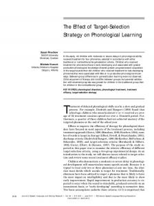
Although there are strong deviations from balanced distributions, the corrected hit probability turns out to be .248, quite close to the theoretical .25. THE PRL AUTOGANZFELD SET DISTRIBUTION As a careful reader may already have noted from Table 1, one of the most remarkable findings in our post-hoc exploration of the random features of the PRL target sequences is the finding that one specific target set was used about three times more often than what can be expected on the basis of chance (see Figure 1). The binomial probability
Notes on Random Target Selection
Page 6
that this set is selected 23 or more times rather than the expected 8.225 times is smaller than 1.25×10⁻⁵.
Figure 1. Distribution of set frequencies in the PRL database, excluding Series 302.
Even if we correct for the fact that this is a post-hoc finding the odds are still very small. Monte Carlo simulations of 100000 experiments with 329 sessions indicate that once in every 2000 experiments a set frequency of 23 or larger occurs. A number of possible scenarios of malfunctioning of the RNG in the random target selection procedure have been considered but none of those results in the extra production of random numbers between 77 and 8. The effect is distributed homogeneously over the different series so it is not connected with a specific experimenter. (Table 4) TABLE 4 RELATIVE FREQUENCY OF SET 20 FOR D IFFERENT SERIES
Series 1 2 3 101 102 103 104/105 201 301
N sessions 22 9 35 50 50 50 56 7 50
Set 20 percentage (MCE = 2.5%) 9.1 0 8.6 4 8 4 7.1 0 12
Another apparently non random feature of the set frequency distribution that springs to the eye of the observer of Figure 1, is that the sets below number 20 are significantly over represented. (t = 4.3, df =38, p = 5.7×10⁻⁵, two-tailed). The sets with a
Notes on Random Target Selection
Page 7
set number smaller than 20 have a mean frequency of 9.26 while sets above 20 have a mean frequency of 6.5. Note that the target set frequency distribution does not figure in any way in the calculation of target hit probability. Deviations in that distribution do not therefore affect the conclusions drawn in the original paper. DISCUSSION Incidental correspondences between target distributions and subject preferences may result in post-hoc hit probabilities that are different from the theoretical. Most notably this effect has been observed in experimental series that use a small set of targets, such as Series 302 of PRL’s autoganzfeld studies. The target preferences coincide with the target distribution and thus result in a post-hoc hit probability of .3408. A proper correction was already made in the original publication (Bem and Honorton, 1994). Also, the preferences of subjects for positions in the judging sequence is quite pronounced, but it turns out that the corrected probabilities are smaller than the theoretical ones. Thus, not taking into account these biases turns out to be a conservative approach for the PRL autoganzfeld series. This holds for dynamic as well as static targets. It also holds for the series 302 separately. The preference for specific targets results in a corrected expected probability which is .2598 and thus indeed should result in an adjustment of the reported z-scores. A conservative estimate of the over-all z-score (calculated from the exact binomial with series 302 excluded) is z = 2.47 rather than the reported z = 2.89. More importantly it turns out that the corrections for static and dynamic sets are quite different. A conservative correction reduces the 10% differential effect to a non-significant 6.8%. Using the miss-based correction which is arguably more appropriate for this internal comparison reduces the differential to a still non-significant 7.4%. Thus, the apparent advantage of the dynamic targets should be considered suggestive at best. The miss-based correction yields an overall corrected expected probability of .2103, which is considerably lower than the theoretical and is associated with z = 4.67. While that would seem highly significant, it would be unwise to accord this result much evidential value because of the reduced overall number of responses. Many target clips ended up with zero probability because the clip had never been selected as a response. Nonetheless, the result suggests that when subjects correctly selected the target clip, they were going against the prevailing bias for the targets. This is similar to findings by Stanford (1969) which indicated that subjects were more likely to score a hit when they went counter to their prevailing biases. As such, it would be advisable to look for similar effects in other ganzfeld data bases. The over-representation in the target set distribution of set 20 cannot be explained through a normal mechanism. Although set 20 seems to have had some special significance in the PRL autoganzfeld experiments, we do not see a way by which this could have contributed to the excess of apparent psi hits. REFERENCES BEM, D. J. (1994). Response to Hyman. Psychological Bulletin, 115, 25–27.
Notes on Random Target Selection
Page 8
BEM, D. J. & HONORTON, C. (1994). Does psi exist? Replicable evidence for an anomalous process of information transfer. Psychological Bulletin, 115, 4–18. HONORTON, C. (1985). Meta-analysis of psi ganzfeld research: A response to Hyman. Journal of Parapsychology, 49, 51–91. HYMAN , R. (1985). The Psi ganzfeld experiment: A critical appraisal. Journal of Parapsychology, 49, 3–49. HYMAN , R. (1994). Anomaly or artifact? Comments on Bem and Honorton. Psychological Bulletin, 115, 19–24. STANFORD , R. G. (1967). Response bias and the correctness of ESP test responses. Journal of Parapsychology, 31, 280–289.
University of Amsterdam (Bierman) Roetersstraat 15 1018 WB Amsterdam, The Netherlands e-mail:
[email protected] Institute for Parapsychology (Broughton) 402 North Buchanan Blvd. Durham, NC 27701 e-mail:
[email protected] Innovative Software Design (Berger) 7027 Settlers Ridge San Antonio, TX 78238 e-mail:
[email protected]
09/05/02 10:01 AM z:\richard\word docs\papers\s20.doc