Oct 15, 2013 ... Dorigo and Di Caro, 1999) ... of variants, optimizations and heuristics, please
consult (Dorigo and Di ..... Caro, G. D. and Dorigo, M. (1998).
Swarm intelligence: Ant Colony Optimisation S Luz
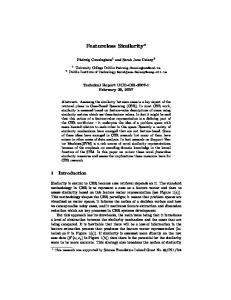
[email protected] October 7, 2014 Simulating problem solving? • Can simulation be used to improve distributed (agent-based) problem solving algorithms? • Yes: directly, in a supervised fashion (e.g. Neural Nets “simulators”) • But also, indirectly, via exploration & experimental parameter tuning • Case Study: Ant Colony Optimisation Heuristics (Dorigo et al., 1996; Dorigo and Di Caro, 1999) • See also (Bonabeau et al., 2000) for a concise introduction (* recommended reading) More specifically, the case study presented in these notes illustrate an application of ant algorithms to the symmetric variant of the traveling salesman problem. Ant algorithms have, as we will see, been employed in a number of optimization problems, including network routing and protein folding. The techniques presented here aim for generality and certain theoretical goals rather than performance in any of these particular application areas. For a good overview of variants, optimizations and heuristics, please consult (Dorigo and Di Caro, 1999). Biological Inspiration • Real ants foraging behaviour
• long branch is r times longer than the short branch. 1
• left graph: branches presented simultaneously. • right graph: shorter branch presented 30 mins. later The gaphs show results of an actual experiment using real ants (Linepithema humile). The role of pheromone plays is clear: it reinforces the ants’ preferences for a particular solution. If regarded as a system, the ant colony will “converge” to a poor solution if the short branch is presented too late (i.e. if the choice of the long branch is reinforced too strongly by the accummulated pheromone). Pheromone trails
A simple model to fit the observed ant behaviour could be based on the probabilities of choices available to ants at the branching point, e.g. the probability that the m + 1th ant to come to the branching point will choose the upper path is given by (Um + k)h (1) Pu (m) = (Um + k)h + (Lm + k)h where Um is the number of ants the chose the upper path, Lm is the number of ants the chose the lower path and h, k are parameters which allow experimenters to tune the model to the observed behaviour, via Monte Carlo simulations. Ants solve TSP • The Travelling Salesman Problem: – Let N = {a, ..., z} be a set of cities, A = {(r, s) : r, s ∈ V } be the edge set, and δ(r, s) = δ(s, r) be a cost measure associated with edge (r, s) ∈ A. – TSP is the problem of finding a minimal cost closed tour that visits each city once. – If cities r ∈ N are given by their coordinates (xr , yr ) and δ(r, s) is the Euclidean distance between r and s, then we have an Euclidean TSP. – If δ(r, s) 6= δ(s, r) for at least one edge (r, s) then the TSP becomes an asymmetric TSP (ATSP).
TSP is known to be NP-hard, with a search space of size 2
(n−1)! . 2
A Simple Ant Algorithm for TSP Initialize while ( ! End condition ) { /∗ c a l l t h e s e ‘ i t e r a t i o n s ’ ∗/ p o s i t i o n each ant on a node while ( ! a l l a n t s b u i l t c o m p l e t e s o l u t i o n ) { /∗ c a l l t h e s e ‘ s t e p s ’ ∗/ f o r ( each ant ) { ant a p p l i e s a s t a t e t r a n s i t i o n r u l e t o incrementally build a solution } } apply l o c a l ( p e r ant ) pheromone update r u l e apply g l o b a l pheromone update r u l e } Characteristics of Artificial Ants • Similarities with real ants: – They form a colony of cooperating individuals – Use of pheromone for stigmergy (i.e. “stimulation of workers by the very performance they have achieved” (Dorigo and Di Caro, 1999)) – Stochastic decision policy based on local information (i.e. no lookahead) Dissimilarities with real ants • Artificial Ants in Ant Algorithms keep internal state (so they wouldn’t qualify as purely reactive agents either) • They deposit amounts of pheromone directly proportional to the quality of the solution (i.e. the length of the path found) • Some implementations use lookahead and backtracking as a means of improving search performance Environmental differences • Artificial ants operate in discrete environments (e.g. they will “jump” from city to city) • Pheromone evaporation (as well as update) are usually problem-dependant • (most algorithms only update pheromone levels after a complete tour has been generated)
3
ACO Meta heuristic 1 2 3 4 5 6 7
1 2 3 4 5 6
acoMetaHeuristic () while ( ! t e r m i n a t i o n C r i t e r i a S a t i s f i e d ) { /∗ b e g i n s c h e d u l e A c t i v i t i e s ∗/ antGenerationAndActivity ( ) pheromoneEvaporation ( ) daemonActions ( ) # optional # } /∗ e n d s c h e d u l e a c t i v i t i e s ∗/
antGenerationAndActivity ( ) while ( availableResources ) { scheduleCreationOfNewAnt ( ) newActiveAnt ( ) }
Ant lifecycle 1 2 3 4 5 6 7 8 9 10 11 12 13 14 15 16 17 18 19
newActiveAnt ( ) i n i t i a l i s e () M := updateMemory ( ) w h i l e ( c u r r e n t S t a t e 6= t a r g e t S t a t e ) { A := r e a d L o c a l R o u t i n g T a b l e ( ) P := t r a n s i t i o n P r o b a b i l i t i e s (A,M, c o n s t r a i n t s ) n e x t := a p p l y D e c i s i o n P o l i c y (P , c o n s t r a i n t s ) move ( n e x t ) i f ( onlineStepByStepPheromoneUpdate ) { depositPheromoneOnVisitedArc ( ) u p d a te R o u t i n g T a bl e ( ) } M := u p d a t e I n t e r n a l S t a t e ( ) } /∗ e n d w h i l e ∗/ i f ( delayedPheromoneUpdate ) { evaluateSolution () depositPheromoneOnAllVisitedArcs ( ) u p d a te R o u t i n g T ab l e ( ) }
How do ants decide which path to take? • A decision table is built which combines pheromone and distance (cost) information: • Ai = [aij (t)]|Ni | , for all j in Ni , where: [τij (t)]α [ηij ]β α β l∈Ni [τil (t)] [ηil ]
aij (t) = P • Ni : set of nodes accessible from i
• τij (t): pheromone level on edge (i, j) at iteration t • ηij =
1 δij
4
(2)
Relative importance of pheromone levels and edge costs • The decision table also depends on two parameters: – α: the weight assigned to pheromone levels – β: the weight assigned to edge costs • Probability that ant k will chose edge (i, j): aij (t) if j has not been visited k Pij (t) = 0 otherwise
(3)
The values given in (3) aren’t strictly speaking correct, since part of the probability mass that would have been assigned to visited nodes is lost. The following variant avoids the problem: aij (t) l∈N k ail (t)
Pijk (t) = P
(4)
i
(for links to non-visited nodes) where Nik ⊆ Ni is the set edges still to be travelled which incide from i. When all edges remain to be travelled, i.e. Nik = Ni , the probability that any edge will be visited next is simply given by the initial decision table: Pijk (t)
=
P
aij (t) aij (t) =P l∈N k ail (t) l∈Ni ail (t) i
=
aij (t) P
[τil (t)] Pl∈Ni l∈Ni
α [η
β il ]
= aij (t)
[τil (t)]α [ηil ]β
Pheromone updating (per ant) • Once all ants have completed their tours, each ant k lays a certain quantity of pheromone on each edge it visited: ( 1 if (i, j) ∈ T k , k k ∆τij (t) = L (t) (5) 0 otherwise • T k (t): ant k’s tour • Lk (t): length of T k (t) Pheromone evaporation and (global) update • Let ∆τij (t) =
m X k=1
– where m is the number of ants, 5
k ∆τij (t)
• and ρ ∈ (0, 1] be a pheromone decay coefficient • The (per iteration) pheromone update rule is given by: τij (t) = (1 − ρ)τij (t0 ) + ∆τij (t)
(6)
where t0 = t − 1 Parameter setting • How do we choose appropriate values for the following parameters? – α: the weight assigned to pheromone levels NB: if α = 0 only edge costs (lengths) will be considered – β: the weight assigned to edge costs NB: if β = 0 the search will be guided exclusively by pheromone levels – ρ: the evaporation rate – m: the number of ants Exploring the parameter space • Different parameters can be “empirically” tested using a multiagent simulator such as Repast • Vary the problem space • Collect statistics • Run benchmarks • etc Performance of ACO on TSP • Ant algorithms perform better than the best known evolutionary computation technique (Genetic Algorithms) on the Asymmetric Travelling Salesman Problem (ATSP) • ... and practically as well as Genetic Algorithms and Tabu Search on standard TSP • Good performance on other problems such as Sequential Ordering Problem, Job Scheduling Problem, and Vehicle Routing Problem Other applications • Network routing (Caro and Dorigo, 1998) and load balancing (Heusse et al., 1998)
6
Application: protein folding in the HP model • Motivation: an important, unsolved problem in molecular biology and biophysics;
• Protein structure, not sequence, determines function. • When folding conditions are met, protein will fold (repeatably) into a native state. Practical applications • Knowing how folding works is important: – Learn how to design synthetic polymers with particular properties – Treat disease (many diseases attributed to protein mis-folding, e.g. Alzheimer disease, cystic fibrosis, mad cow disease etc) • Why model? – Deducing 3-d structure from protein sequence using experimental methods (such as x-ray diffraction studies or nuclear magnetic resonance [NMR]) is highly costly in terms of labour, skills and machinery. • A connection with (serious) games:
7
– Fold.it: A Protein folding game... ACO for Protein Folding: Motivation • Levinthal’s paradox: how can proteins ‘find’ their correct configuration (structure) when there is an astronomical number of configurations they can assume?
49
48 46
50
47
37
38
45
35
36
39
40
43
34
33
32
41
42
31
17
18
16
19
20
21
30
14
15
2
3
22
29
13
12
1
4
23
28
27
10
11
6
5
24
25
26
9
8
7
44
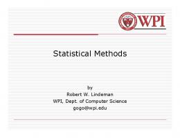
• The HP (hydrophobic-hydrophilic, or nonpolar-polar) model (Dill et al., 1995) restricts the degrees of freedom (for folding) but...
Total energy of this embedding = −19 ; theoretical lower bound = −25
• (Crescenzi et al., 1998; Berger and Leighton, 1998) independently proved folding in simple models (such as the 2D and 3D lattice HP model) to be NP-complete.
A possible ACO approach • There are many ways to implement the HP model; one might adopt the following (Roche & Luz, unpublished): • Problem data: A binary string of length n, representing chain of amino acid residues that make up a protein. • Decision tree: From a given position (in the problem data), valid choices are Left, Right and Forward (orientation) – except where a dead-end is encountered (ie. tour must be self avoiding) • Environment:Pheromone represents a memory of fitness for possible decisions. – e.g. a 2-dimensional array of size [n−1][3], representing the respective desirabilities for the different orientations (left,right,forward) from a given position in the problem data. • Tour: The set of moves (orientations) made by an ant in deriving a partial or complete solution.
8
Ant behaviour • State transition rule: How ant selects next move (left,right,forward) – Exploitation: ∗ Greedy algorithm involve a lookahead (r ≥ 2) to gauge local benefit of choosing a particular direction (benefit measured in terms of additional HH contacts) ∗ Combine greedy algorithm with ‘intuition’ (pheromone), to derive overall cost measure – Exploration: Pseudo-random (often biased) selection of an orientation (help avoid local minima) – Constraints: ∗ Resultant tour must be self avoiding. ∗ Look-ahead could help detect unpromising folding (e.g. two elements can be topological neighbours only when the number of elements between them is even etc) Pheromone update • Local update: (optional) – Can follow same approach as with TSP, by applying pheromone decay to edges as those edges are visited, to promote the exploration of different paths by subsequent ants during this iteration. • Global update: – Can also follow same approach as with TSP: Apply pheromone decay (evaporation!) to each edge in the decision tree (negative factor) – Selection of ‘best’ candidate (best cost) and reinforcement of pheromone on edges representing this decision – Typically global updating rule will be iteration-best or global-best Results • Competitive with best-known algorithms (MCMC, GA, etc) in terms of best conformations found • Can be slow and more resource-intensive. • May be possible to combine ACO with techniques useb by approximation algorithms (Hart and Istrail, 1995) • Alternative approaches based on ACO have been proposed (Shmygelska and Hoos, 2003).
9
References Berger, B. and Leighton, T. (1998). Protein folding in the hydrophobichydrophilic (hp) is np-complete. In Proceedings of the second annual international conference on Computational molecular biology, pages 30–39. ACM Press. Bonabeau, E., Dorigo, M., and Theraulaz, G. (2000). Inspiration for optimization from social insect behaviour. Nature, 4006. Caro, G. D. and Dorigo, M. (1998). Antnet: Distributed stigmergetic control for communications networks. Journal of Artificial Intelligence Research, 9:317–365. Crescenzi, P., Goldman, D., Papadimitriou, C., Piccolboni, A., and Yannakakis, M. (1998). On the complexity of protein folding (abstract). In Proceedings of the second annual international conference on Computational molecular biology, pages 61–62. ACM Press. Dill, K. A., Bromberg, S., Yue, K., Fiebig, K. M., Yee, D. P., Thomas, P. D., and Chan, H. S. (1995). Principles of protein folding – A perspective from simple exact models. Protein Science, 4(4):561–602. Dorigo, M. and Di Caro, G. (1999). The ant colony optimization meta-heuristic. In Corne, D., Dorigo, M., and Glover, F., editors, New Ideas in Optimization, pages 11–32. McGraw-Hill, London. Dorigo, M., Maniezzo, V., and Colorni, A. (1996). The Ant System: Optimization by a colony of cooperating agents. IEEE Transactions on Systems, Man, and Cybernetics Part B: Cybernetics, 26(1):29–41. Hart, W. E. and Istrail, S. (1995). Fast protein folding in the hydrophobichydrophilic model within three-eights of optimal. In Proceedings of the twenty-seventh annual ACM symposium on Theory of computing, pages 157–168. ACM Press. Heusse, M., Guerin, S., Snyers, D., and Kuntz, P. (1998). Adaptive agent-driven routing and load balancing in communication networks. Adv. Complex Systems, 1:237–254. Shmygelska, A. and Hoos, H. H. (2003). An improved ant colony optimisation algorithm for the 2D HP protein folding problem. In Xiang, Y. and Chaibdraa, B., editors, Advances in Artificial Intelligence: 16th Conference of the Canadian Society for Computational Studies of Intelligence, volume 2671 of Lecture Notes in Computer Science, pages 400–417, Halifax, Canada. Springer-Verlag.
10