arXiv:quant-ph/9809075v2 13 Dec 1998. NP PROBLEM IN QUANTUM ALGORITHM. Masanori Ohya and Natsuki Masuda. Science University of Tokyo.
arXiv:quant-ph/9809075v2 13 Dec 1998
NP PROBLEM IN QUANTUM ALGORITHM Masanori Ohya and Natsuki Masuda Science University of Tokyo Noda City, Chiba 278-8510, JAPAN Abstract In complexity theory, there exists a famous unsolved problem whether NP can be P or not. In this paper, we discuss this aspect in SAT (satisfiability) problem, and it is shown that the SAT can be solved in plynomial time by means of quantum algorithm.
1
Introduction
Although the ability of computer is highly progressed, there are several problems which may not be solved effectively, namely, in polynomial time. Among such problems, NP problem and NP complete problem are fundamental. It is known[5] that all NP complete problems are equivalent and an essential question is whether there exists an algorithm to solve a NP complete problem in polynomial time. After pioneering works of Feymann[4] and Deutsch[1], several important works have been done on quantum algorithms by Deutsch and Josa[2], Shor[7], Ekert and Josa[3] and many others[6]. The computation in quantum computer is performed on a tensor product Hilbert space, and its fundamental point is to use quantum coherence of states. All mathematical features of quantum computer and computation are summarized in [6]. In this paper, we discuss the quantum algorithm of the SAT problem and point out that this problem, hence all other NP problems, can be solved in polynomial time by quantum computer if the superposition of two orthogonal vectors |0i and |1i is physically detected.
1
2
SAT Problem
Let X ≡ {x1 , · · · , xn } be a set. Then xk and its negation xk (k = 1, 2, · · · , n) are called literals and the set of all such literals is denoted by ′ ′ ′ X = {x1 , x1 , · · · , xn , xn }. The set of all subsets of X is denoted by F (X ) ′ and an element C ∈ F (X ) is called a clause. We take a truth assignment to all variables xk . If we can assign the truth value to at least one element of C, then C is called satisfiable. When C is satisfiable, the truth value t(C) of C is regarded as true, otherwise, that of C is false. Take the truth values as ”true↔ 1, false↔ 0”. Then C is satisfiable iff t(C) = 1. Let L = {0, 1} be a Boolean lattice with usual join ∨ and meet ∧, and t(x) be the truth value of a literal x in X. Then the truth value of a clause C is written as t(C) ≡ ∨x∈C t(x). Moreover the set C of all clauses Cj (j = 1, 2, · · · m) is called satisfiable iff the meet of all truth values of Cj is 1; t(C) ≡ ∧m j=1 t(Cj ) = 1. Thus the SAT problem is written as follows: Definition 1. SAT Problem: Given a set X ≡ {x1 , · · · , xn } and a set C = {C1 , C2 , · · · , Cm } of clauses, determine whether C is satisfiable or not. That is, this problem is to ask whether there exsits a truth assignment to make C satisfiable. It is known[5] in usual algorithm that it is polynomial time to check the satisfiability only when a specific truth assignment is given, but we can not determine the satisfiability in polynomial time when an assignment is not specified.
3
Quantum Algorithm of SAT
Let 0 and 1 of the Boolean lattice L be denoted by the vectors |0i ≡ !
1 0
!
0 and |1i ≡ in the Hilbert space C2 , respectively. That is, the vector 1 |0i corresponds to falseness and |1i does to truth. As we explained in the previous section, an element x ∈ X can be denoted by 0 or 1, so by |0i or |1i . In order to describe a clause C with at most n 2
length by a quantum state, we need the n-tuple tensor product Hilbert space H ≡ ⊗n1 C2 . For instance, in the case of n = 2, given C = {x1 , x2 } with an assignment x1 = 0 and x2 = 1, then the corresponding quantum state vector is |0i ⊗ |1i , so that the quantum state vector describing C is generally written by |Ci = |x1 i ⊗ |x2 i ∈ H with xk = 0 or 1 (k=1,2). The quantum computation is performed by a unitary gate constructed from several fundamental gates such as Not gate, Controlled-Not gate, Controlled-Controlled Not gate [3, 6]. Once X ≡ {x1 , · · · , xn } and C = {C1 , C2 , · · · , Cm } are given, the SAT is to find the vector |f (C)i ≡ ∧m j=1 ∨x∈Cj t(x), where t(x) is |0i or |1i when x = 0 or 1, respectively, and t(x) ∧ t(y) ≡ t(x ∧ y), t(x) ∨ t(y) ≡ t(x ∨ y). We consider the quantum algorithm for the SAT problem. Since we have n variables xk (k = 1, · · · n) and a quantum computation produces some dust bits, the assignments of the n variables and the dusts are represented by n qubits and l qubits in the Hilbert space ⊗n1 C2 ⊗l1 C2 . Moreover the resulting state vector |f (C)i should be added, so that the total Hilbert space is H ≡ ⊗n1 C2 ⊗l1 C2 ⊗ C2 . Let us start the quantum computation of SAT problem from an initial vector |v0 i ≡ ⊗n1 |0i⊗l1 |0i⊗|0i when C contains n Boolean variables x1 , · · · xn . We ! 1 1 n √1 apply the discrete Fourier transformation denoted by UF ≡ ⊗1 2 1 −1 to the part of the Boolean variables of the vector |v0 i , then the resulting state vector becomes 1 |vi ≡ UF ⊗l1 I |v0 i = √ n ⊗n1 (|0i + |1i) ⊗l1 |0i ⊗ |0i , 2 where I is the identity matrix in C2 . This vector can be written as 1 |vi = √ n 2
1 X
x1 ,···,xn =0
⊗nj=1 |xj i ⊗l1 |0i ⊗ |0i .
Now, we perform the quantum computer to check the satisfiability, which will be done by a unitary operator Uf properly constructed by unitary gates. Then after the computation by Uf , the vector |vi goes to 1 |vf i ≡ Uf |vi = √ n 2
1 X
x1 ,···,xn =0
3
Uf ⊗nj=1 |xj i ⊗l1 |0i ⊗ |0i
1 = √ n 2
1 X
x1 ,···,xn =0
⊗nj=1 |xj i ⊗li=1 |yi i ⊗ |f (x1 , · · · , xn )i ,
where f (x1 , · · · , xn ) ≡ f (C) because C contains x1 , · · · xn , and |yi i are the dust bits produced by the computation. As we will explain in an example below, the unitary operator Uf is concretely constructed. The final step to check the satisfiability of C is to apply the projection E ≡ ⊗1n+l I ⊗|1i h1| to the state |vf i , mathematically equivalent , to compute the value hvf | E |vf i . If the vector E |vf i exists or the value hvf | E |vf i is not 0, then we conclude that C is satisfiable.The value of hvf | E |vf i corresponds to that of the ramdom algorithm as we will see in an example of the next section and it may or may not be obtained in polynominal time. Let us consider an operator Vθ , given by Vθ ≡ ⊗1n+l (A |0i h0| + B |1i h1|) ⊗ eiθf (C) I, !
1 1 1 1 and B ≡ √12 and apply it to the vector |vf i , where A ≡ √12 1 −1 −1 1 and θ is a certain constant describing the phase of the vector |f (C)i . The resulting vector is the superposition of two vectors with some constants α, β such as Vθ |vf i = √
1 2n+l
�
�
⊗1n+l (|0i + |1i) ⊗ α |0i + βeiθ |1i ,
one of which is polarized with θ and another is non-polarized. The existence of the mixture of two vectors |0i and eiθ |1i is a starting point of quantum computation, which implies the satisfiability.
4
Example of Computation
Let us explain the quantum computation for SAT in tha case X = {x1 , x2 , x3 } and C = {{x1 } , {x2 , x3 } , {x1 , x3 } , {x1 , x2 , x3 }} . The resulting state |f (x1 , x2 , x3 )i is written as |f (x1 , x2 , x3 )i = |x1 i ∧ (|x2 i ∨ |x3 i) ∧ (|x1 i ∨ |x3 i) ∧ (|x1 i ∨ |x2 i ∨ |x3 i) In the quantum computation, it is not necessary to substitute all values of xj (j = 1, 2, 3) as the classical computation, we have only to use a unitary 4
!
operator Uf for the computation of |f (x1 , x2 , x3 )i . This unitary operator Uf is constructed as follows: Let UN OT , UCN and UCCN be Not gate on C2 , Controlled-Not gate on C2 ⊗ C2 and Controlled-Controlled-Not gate on C2 ⊗ C2 ⊗ C2 , respectively, which are given by UN OT = |0i h1| + |1i h0| UCN = |0i h0| ⊗ I + |1i h1| ⊗ (|0i h1| + |1i h0|) UCCN = |0i h0| ⊗ |0i h0| ⊗ I + |0i h0| ⊗ |1i h1| ⊗ I + |1i h1| ⊗ (|0i h0| ⊗ |1i h0|) Then the unitary operator Uf is determined by the combination of the above three unitaries as Uf ≡ U36 U35 · · · U2 U1 , where, for instance, 2 20 U1 ≡ |0i h0| ⊗23 1 I + |1i h1| ⊗1 I ⊗ (|0i h1| + |1i h0|) ⊗1 I 2 19 U2 ≡ I ⊗ |0i h0| ⊗22 1 I + I ⊗ |1i h1| ⊗1 I ⊗ (|0i h1| + |1i h0|) ⊗1 I 2 2 18 U3 ≡ ⊗21 I ⊗ |0i h0| ⊗21 1 I + ⊗1 I ⊗ |1i h1| ⊗1 I ⊗ (|0i h1| + |1i h0|) ⊗1 I
and other U4 , · · · , U36 are similarly constructed (see the computation diagram 1). In this case, we need 20 dust bits (the number of the dust bits needed in a general case is counted in the next section), so that Uf is operated on the 2 Hilbert space ⊗24 1 C . Starting from the initial vector |v0 i ≡ ⊗31 |0i ⊗20 1 |0i ⊗ |0i , the final vector is |vf i = U36 · · · U1 UF |v0 i = Uf UF |v0 i 1 = √ (|0, 0, 0, 0, 1, 1, 0, 1, 0, 1, 0, 0, 0, 1, 1, 0, 0, 0, 1, 1, 1, 0, 1; 0i 23 + |1, 0, 0, 1, 1, 1, 0, 0, 0, 1, 1, 0, 0, 1, 1, 1, 0, 0, 1, 1, 1, 0, 1; 0i + |0, 1, 0, 0, 0, 1, 1, 1, 0, 1, 0, 1, 0, 1, 1, 0, 1, 0, 1, 1, 1, 0, 1; 0i + |0, 0, 1, 0, 1, 0, 1, 1, 1, 0, 0, 0, 0, 0, 1, 0, 1, 0, 0, 1, 0, 0, 0; 0i + |1, 1, 0, 1, 0, 1, 1, 0, 0, 1, 1, 1, 1, 1, 0, 1, 1, 1, 1, 1, 0, 1, 0; 0i + |1, 0, 1, 1, 1, 0, 1, 0, 1, 1, 1, 0, 0, 0, 1, 1, 1, 1, 1, 1, 1, 1, 1; 1i + |0, 1, 1, 0, 0, 0, 1, 1, 1, 0, 0, 1, 0, 0, 1, 0, 1, 0, 0, 1, 0, 0, 0; 0i + |1, 1, 1, 1, 0, 0, 1, 0, 1, 1, 1, 1, 1, 0, 1, 1, 1, 1, 1, 1, 1, 1, 1; 1i) , 5
where we used the notation |x1 , x2 , x3 , y1 , · · · , y20 ; f (x1 , x2 , x3 )i ≡ ⊗3j=1 |xj i ⊗20 i=1 |yi i ⊗ |f (x1 , x2 , x3 )i Applying the operator Vθ of the previous section to the vector |vf i , we obtain √ 1 3 1 23 √ |0i + eiθ |1i), ⊗1 (|0i + |1i) ⊗ ( 2 2 223 which is the superposition of two vectors |0i and the polarized vector |f (C)i = |1i . Moreover when we measure the operator E ≡ ⊗23 1 I ⊗ |1i h1| in the state Vθ |vf i , we obtain 1 hvf Vθ | E |Vθ vf i = . 4 These conclude the satisfiability of C. x1
x2
x3
f (x1 , x 2 , x3 )
6
5
Complexity of Quantum Algorithm for SAT
Here we discuss the number of steps for the quantum algorithm of the SAT problem. The size of input with n variables xk and their negations xk (k = 1, · · · , n)and also C = {C1 , · · · , Cm } is N1 = log n + 2mn like the classical algorithm because |Ck | , the number of the elements in Ck , is at most n, so that it is the polynominal order (O(mn)). The number of the dust bits to compute f (C) is caused from that of the operations and substitutions of AND and OR, so that the maximum number (complexity) N2 of the dust bits needed is the same as that of the classical case, namely, N2 = (the numbers of AND and OR operations )− (the steps to take the negation) = (5mn − 1) − mn = 4mn − 1. The steps N3 needed to obtain the vector |f (C)i is counted as follows: Fisrt take 1 step for the discrete Fourier transform to get the entangled vector, and we need 3mn steps for truth assignment and substitution to n variables. Secondly to compute the logical sum in each clause and take their logical product, the complexity corresponding to the logical sum, whose gate is made from four unitaries, is 4m(2n − 1) and that corresponding to the logical product is m − 1. Thus N3 = 1 + 3mn + 4m(2n − 1) + m − 1 = 11mn − 3m. Finally to check the satisfiability of C, we have to look at the situation of |f (C)i registered at the last position of the tensor product state such as the last position of physical registers (e.g., spins) lined up. This can be easily done by applying the operator Vθ to |vf i , and the resulting vector is a superposition of two vectors |0i and eiθ |1i . We can obtain in polynominal time (at most n + l + 1) the vector |Vθ vf i and the value of < Vθ vf , EVθ vf >= |β|2 for the projection E if needed. The existence of the above superposition is a starting point of quantum computation, so that it should be physically detected being different from both |0i and |1i , which implies the satisfiability. Thus the quantum algorithm of the SAT problem is in polynominal order.
Acknowledgment: One of the authors (MO) appreciate Professor A. Ekert for his critical reading and valuable comments.
References
7
[1] D. Deutsch, Quantum theory, the Church-Turing principle and the universal quantum computer, Proc. of Royal Society of London series A, 400, pp.97-117, 1985. [2] D. Deutsch and R. Jozsa, Rapid solution of problems by quantum computation, Proc. of Royal Society of London series A, 439, pp.553-558, 1992. [3] A. Ekert and R.Jozsa, Quantum computation and Shor’s factoring algorithm, Reviews of Modern Physics, 68 No.3,pp.733-753, 1996. [4] R. Feymann, Quantum mechanical computer, Optics News, 11 ,pp.11-20, 1985. [5] M. Garey and D. Johnson, ”Computers and Intractability - a guide to the theory of NP-completeness”, Freeman, 1979. [6] M. Ohya,“Mathematical Foundation of Quantum Computer”, “Mathematical Foundation of Quantum Information”, Maruzen Publ. Company, 1998 [7] P.W. Shor, Algorithm for quantum computation : Discrete logarithm and factoring algorithm, Proceedings of the 35th Annual IEEE Symposium on Foundation of Computer Science, pp.124-134, 1994.
8