Nucleon form factors and structure functions from Lattice QCD

DESY 01-110 August 2001

NUCLEON FORM FACTORS AND STRUCTURE FUNCTIONS FROM LATTICE QCD∗

arXiv:hep-ph/0108105v1 12 Aug 2001

1 ¨ M. GOCKELER , R. HORSLEY2 , D. PLEITER2 , P. E. L. RAKOW1 , G. SCHIERHOLZ2,3 1

Institut f¨ ur Theoretische Physik, Universit¨ at Regensburg, D-93040 Regensburg, Germany 2

John von Neumann-Institut f¨ ur Computing NIC, Deutsches Elektronen-Synchrotron DESY, D-15735 Zeuthen, Germany 3

Deutsches Elektronen-Synchrotron DESY, D-22603 Hamburg, Germany

In this talk we highlight recent lattice calculations of the nucleon form factors and structure functions.

1

Introduction

The lattice formulation of QCD is, at present, the only known way of obtaining low energy properties of the theory in a direct way, without any model assumptions. Quantities within the grasp of lattice QCD involving light quarks include the hadron mass spectrum, quark masses, the Λ parameter, the chiral condensate, the sigma term, decay constants, the axial and tensor charge of the nucleon, form factors and twist two and four polarised and unpolarised moments of structure functions for the nucleon, pion and rho, to name only a few of the possibilities. Our group (the QCDSF collaboration) has been actively involved for the last few years in attempting to determine some of these quantities, all characterised by their non-perturbative nature. Rather than giving an exhaustive progress report of recent developments in the field1 we shall, due to lack of space, focus our attention on two topics: nucleon form factors (including the axial charge) and moments of structure functions and how the lattice method can lead to their determination. The lattice approach involves first euclideanising the QCD action and then discretising space-time (with lattice spacing a). The path integral then becomes a very high dimensional partition function, which is amenable to Monte Carlo methods of statistical physics. This allows correlation functions (which can be related to QCD matrix elements) to be determined. Progress ∗ Talk given by G. Schierholz at ‘Workshop on Lepton Scattering, Hadrons and QCD’, Adelaide University, March 26 - April 6, 2001.

Talk to be published by World Scientific Publishing Co.

1

in the field is slow. First our ‘box’ must be large enough to fit our correlation functions into. Then, often, a chiral extrapolation must be made from a quark mass region around the strange quark mass to the light up and down quarks. Finally the continuum limit must be taken, i.e. a → 0. This is all very time consuming as, in the statistical mechanics picture, we are approaching a second order phase transition, with all its attendant problems. Additionally, simply to save computer time, the fermion determinant in the action is often discarded. This ‘quenched’ or ‘valence’ procedure is an uncontrolled approximation. Recently, however, simulations with two mass-degenerate sea quarks have begun appearing, allowing a first look at the possible effects of quenching. Finally, in addition to the above problems, to be able to compare with phenomenological or experimental results, matrix elements must be renormalised. In total this is an ambitious programme. 2 2.1

Generalities The processes

Lepton–nucleon elastic scattering, lN → lN , in which a photon is exchanged between the lepton (usually an electron) and the nucleon (usually a proton), has been studied for many years. Indeed there has been a resurgence of interest in these processes as part of the Jefferson Laboratory (Jlab) ‘hadron’ physics programme. The scattering matrix element can be decomposed into a known electromagnetic piece and an unknown QCD matrix element with decomposition:   qν p ′ , s~ ′ ) γ µ F1 (Q2 ) + iσ µν hN (~ p ′ , s~ ′ )|J µ (~ q )|N (~ p, ~s)i = u(~ F2 (Q2 ) u(~ p, ~s) , 2mN (1) where q = p′ − p is the momentum transfer and Q2 = −q 2 > 0. The values at Q2 = 0 are F1p (0) = 1 due to the conservation of the vector current and F2p (0) = µp − 1, the anomalous magnetic moment, in units of e/2mN or magnetons. (F1n (0) = 0, F2n (0) = µn .) Experimentally, it is more convenient to define the Sachs form factors Q2 F2 (Q2 ) , Ge (Q2 ) = F1 (Q2 ) − (2mN )2 Gm (Q2 ) = F1 (Q2 ) + F2 (Q2 ) . Earlier experimental results give phenomenological (dipole) fits of −2  Gn (Q2 ) Q2 Gp (Q2 ) = mn = 1+ 2 , Gne (Q2 ) = 0 , Gpe (Q2 ) = m p µ µ mV

Talk to be published by World Scientific Publishing Co.

(2)

2

with mV ≈ 0.82 GeV, µp ≈ 2.79 and µn ≈ −1.91. Similarly neutrino–nucleon scattering, for example νµ n → µ− p mediated by a W + exchange, leads to an unknown axial current hadronic matrix element between neutron and proton states, which, with the use of current algebra and isospin invariance, may be re-written between p states alone and has Lorentz decomposition   qµ ′ ′ 2 2 hp(~ p ′ , s~ ′ )|Au−d (~ q )|p(~ p , ~ s )i = u(~ p , s ~ ) γ γ g (Q ) + iγ h (Q ) u(~ p, ~s) µ 5 A 5 A µ 2mN (3) where Au−d = uγµ γ5 u − dγµ γ5 d. Experimental results give phenomenological µ fits −2  Q2 2 , (4) gA (Q ) = gA (0) 1 + 2 mA with mA ≈ 1.00 GeV. From the β decay we know2 gA ≡ gA (0) = 1.2670(35). At higher momentum transfer, the nucleon is broken up by the photon (or W ± ) probe. We enter the regime of deep inelastic scattering experiments eN → eX (or νµ n → µ− X). The operator product expansion, OPE, leads to relations between moments of the structure functions and certain nucleon matrix elements. For example, Z 1 1 µ2 1 (5) dxxn−2 F2 (x, Q2 ) = EnM S ( 2 , g M S )vnM S (g M S ) + O( 2 ) . 3 Q Q 0 Here x is the Bjorken variable and vnM S ∝ hN |On |N iM S , where On ∼ qγµ1 Dµ2 . . . Dµn q are operators bilinear in the quarks, each containing n − 1 covariant derivatives. For eN scattering only even moments contribute, while for νN all moments are allowed. All the matrix elements briefly discussed above can be determined nonperturbatively using lattice QCD. 2.2

Lattice Technicalities

The general method of determining matrix elements is by forming ratios of three-point to two-point correlation functions: Rαβ (t, τ ; p~) =

hNα (t; p~)O(τ ; ~0)N β (0; p~)i , hN (t; p~)N (0; ~p)i

(6)

where N is the three quark baryon operator and O is a bilinear quark operator. Provided that t ≫ τ ≫ 0, then R can be shown to be directly proportional to the matrix element hN |O|N i. (R may be easily generalised to allow for

Talk to be published by World Scientific Publishing Co.

3

momentum transfer.) If we re-write the numerator of eq. (6) using quark propagators, we see that we have two classes of diagrams: one in which the inserted operator is attached to quark propagators to the nucleon, and a second class where the quark propagator from the operator is disjoint from the baryon. In this second class the interactions between the inserted operator and the baryon take place only via gluon exchange. Numerically, due to large ultra-violet fluctuations, no useful signal is seen. So either we must presently assume that their effects are small, or calculate ‘non-singlet’ (i.e. u−d) matrix elements where these second class terms cancel. The matrix elements must be renormalised. There are several possibilities. We may simply consider a ratio of matrix elements between different hadronic states, so that the renormalisation constant cancels. However, this is not very useful. The axial and vector renormalisation constants (the currents being partially conserved) may be determined by demanding that their (continuum) Ward Identities are obeyed, which produces non-perturbative renormalisation constants. (Incidently they are also renormalisation scheme independent.) Perturbation theory can be applied, but due to technical problems only one loop results are known. Even with this restriction, perturbation theory can be improved leading to ‘tadpole improved’ or TI perturbation theory. However it still suffers from unknown systematic errors. The ALPHA Collaboration has developed techniques3 allowing some renormalisation constants to be determined by stepping up from a low energy scale to a high energy scale where the Z can be matched to (known) perturbation theory. Finally one can attempt to ‘mimic’ the perturbation theory method by calculating the operator numerically between quark states in the Landau gauge. Also note that it is desirable to make the errors in the determination to be of O(a2 ) rather than O(a), because then the approach to the continuum is faster4 . This introduces further irrelevant operators, with ‘improvement’ coefficients which also must be determined. At present, for the axial and vector currents most renormalisation constants and improvement coefficients are known non-perturbatively. For vn we rely on TI perturbation theory. 3 3.1

Results The Axial Charge

Using the quenched approximation we have made simulations at three lattice spacings: a = 0.093, 0.068 and 0.051 fma . For each lattice size simulations are a Corresponding

to a−1 = 2.12, 2.90 and 3.85 GeV, with scale5 r0 = 0.5 fm.

Talk to be published by World Scientific Publishing Co.

4

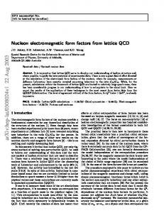
made at four or more quark masses, which are then linearly extrapolated to the chiral limit. (A picture for vn will be shown later in section 3.3.) We also have one unquenched result at a ≈ 0.11 fm. In Fig. 1 we show all these numbers6 . The results all lie somewhat lower than the experimental value, and at present 1.30

gA 1.20

quenched 1.10

dynamical

1.00

0.90

0.00

0.01

0.02 2 (a/r0)

0.03

0.04

0.05

Figure 1. The continuum extrapolation of gA .

there is no clear difference between quenched and unquenched fermions. (Note that for the quenched results, this is a fully non-perturbative calculation; for the unquenched result, there is still a little uncertainty.) While it is possible to extrapolate the quenched data to the continuum limit (although it would be very desirable to have more points because the noise is uncomfortably large at present), we see that we are only at the beginning of obtaining results with dynamical fermions. 3.2

Form Factors

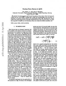
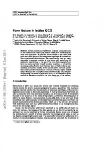
In Fig. 2 we show proton electric and magnetic form factors7 , for our quenched lattice a = 0.068fm. Other lattice values and the unquenched results are very similar. Due to the momentum transfer the results are rather noisy. However the present trend is clear: the dipole fit gives values of mV too large in comparison with the phenomenological value. This is confirmed in √ Fig. 3. For the nucleon we find rrms ≡ 12/mV ≈ 0.60 fm in the quenched approximation and rrms ≈ 0.70 fm for the dynamical case. This is to be compared with the phenomenological value rrms = 0.83 fm. Perhaps the ‘pion

Talk to be published by World Scientific Publishing Co.

5

3.0

2.5 p

2

G m(Q )

2.0

1.5

1.0

0.5 p

2

G e(Q ) 0.0 0.0

0.5

1.0

1.5 2 2 Q [GeV ]

2.0

2.5

3.0

Figure 2. Gpe and Gpm compared to experimental data for quenched fermions at a = 0.068fm. 1.25

1.00

quenched

mV [GeV]

dynamical phenom

0.75

0.50

Ge

mV

0.00

0.01

0.02 2 (a/r0)

0.03

0.04

0.05

e Figure 3. mG compared to its phenomenological value. V

cloud’ has not developed at our dynamical quark masses, which makes the nucleon appear to be smaller than it really is. µp is roughly consistent with m the phenomenological value (but with large errors), while mG is again too V

Talk to be published by World Scientific Publishing Co.

6

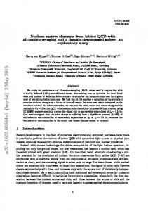
large. The recent Jlab results8 for Gpe /Gpm indicate a functional difference between the electric and magnetic form factors. This is shown in Fig. 4. If 0.5 p

2

p

2

G e(Q )/G m(Q ) 0.4

µP =2.79 −1

−1

0.3

Jlab Experiment Lattice

0.2

0.1

0.0

0.5

1.0

1.5 2 2 Q [GeV ]

2.0

2.5

3.0

Figure 4. Gpe /Gpm compared to experimental data for quenched fermions at a = 0.068fm.

eq. (2) holds then the ratio of form factors should be constant. Unfortunately at present the lattice data is too noisy to draw any conclusion. Finally in Fig. 5 we show the axial form factor. Again the previous comments as for Gpe , Gpm hold verbatim. 3.3

Moments of the nucleon structure function

Some years ago, we published our first results9 for vn , n = 1, 2, 3. The re(d)M S (u)M S − vn is shown again in Fig. 6. for unimproved Wilplotted data for vn son fermions. A comparison is made with MRS phenomenological results10 . While higher moments tend to agree (although large error bars might hide any discrepancy), it seems that there is a discrepancy for the lowest moment. This may be due to renormalisation and discretisation effects, higher-twist contributions, the chiral extrapolation11, or perhaps the phenomenological distribution functions, being global fits, do not fit this moment very well. Naively this resultP is also perhaps expected as v2 is part of the energy-momentum sum rule, v2valence + v2sea = 1, and due to quenching the sea contribution is reduced. For higher moments this is less of an effect, as the gluon contribution is more important for smaller x.

Talk to be published by World Scientific Publishing Co.

7

1.50

1.25 2

gA(Q )

1.00

0.75

0.50

0.25

0.00 0.0

0.5

1.0

1.5 2 2 Q [GeV ]

2.0

2.5

3.0

p Figure 5. gA compared to experimental data for quenched fermions at a = 0.068fm.

0.4 √2mK

mπ

__ MS, µ=2GeV

0.3

n=1 0.2

0.1 n=2 n=3 0

0.00

2.00

4.00 6.00 2 2 (r0/a) x (amps) (u)M S

8.00

10.00

(d)M S

− vn for quenched fermions at a = Figure 6. The chiral extrapolation for vn 0.093fm (circles), compared to the MRS fit function10 (filled squares). The dot-dashed lines show the positions of mπ and a (hypothetical) strange quark pseudoscalar particle.

First let us look at the experimental data. The cleanest direct determina(u)M S (d)M S tion of vn − vn is given from the F2p − F2n NMC data12 , as shown in

Talk to be published by World Scientific Publishing Co.

8

0.150 MRS

2

F2 (x,Q =4GeV ) − F2 (x,Q =4GeV )

0.125

n

2

0.100

2

0.075

p

2

0.050

0.025

0.000

0

0.2

0.4

0.6

0.8

1

x

Figure 7. The experimental binned data for F2p − F2n at Q2 = 4GeV2 from the NMC Collaboration12 compared with the MRS parton fit function 10 .

Fig. 7, because the one experiment uses both p and n targets. Note that there is a paucity of data at large x ∼ 1, which is the region where the moments are most sensitive to. (We make a simple linear extrapolation from the largest data point to x = 1.) While the MRS fit does not quite follow the data, the (u)M S (d)M S area under the curve ∝ v2 − v2 is about the same, so there is indeed no problem. Secondly we have investigated the continuum extrapolation for the lowest moment, in Fig. 8 using improved fermions. Surprisingly, perhaps, there seems to be little a2 trend in the data (c.f. this with gA , Fig. 1). Thus the previous discrepancy still holds. Acknowledgements The unquenched configurations were generated in collaboration with UKQCD Collaboration. The propagators were computed using the T3E at ZIB and the APE100 at NIC (Zeuthen). References 1. A good source of information is: Proceedings of the XVIIIth International Symposium on Lattice Field Theory, Bangalore, India, editors T.

Talk to be published by World Scientific Publishing Co.

9

0.30

0.25

0.20

0.15

__ MS, µ=2GeV

0.00

0.01

0.02 2 (a/r0)

0.03

0.04

(u)M S

Figure 8. The continuum extrapolation for v2

2. 3. 4. 5. 6. 7.

8. 9. 10. 11. 12.

(d)M S

− v2

.

Bhattacharya, R. Gupta and A. Patel, Nucl. Phys. Proc. Suppl. 94 (2001). Review of Particle Physics, D. E. Groom et al, Eur. Phys. Jour. C15 (2000) 1. R. Sommer, Schladming Lectures (1997), hep-ph/9711243. M. L¨ uscher, Les Houches Lectures (1997), hep-ph/9711205. M. Guagnelli, R. Sommer and H. Wittig, Nucl. Phys. B535 (1998) 389, hep-lat/9806005. R. Horsley, Lattice 2000, Nucl. Phys. Proc. Suppl. 94 (2001) 307, heplat/0010059. S. Capitani, M. G¨ ockeler, R. Horsley, B. Klaus, H. Oelrich, H. Perlt, D. Petters, D. Pleiter, P. E. L. Rakow, G. Schierholz, A. Schiller and P. Stephenson, Nucl. Phys. Proc. Suppl. 73 (1999) 294, hep-lat/9809172. M. K. Jones et al., Phys. Rev. Lett. 84 (2000) 1398, nucl-ex/9910005. M. G¨ ockeler, R. Horsley, E.-M. Ilgenfritz, H. Perlt, P. Rakow, G. Schierholz and A. Schiller, Phys. Rev. D53 (1996) 2317, hep-lat/9508004. A. Martin, R. G. Roberts and W. J. Stirling, Phys. Lett. B354 (1995) 155, hep-ph/9502336. W. Detmold, W. Melnitchouk, J. W. Negele, D. B. Renner and A. W. Thomas, hep-lat/0103006. A. Arneodo et al., Phys. Rev. D50 (1994) R1.

Talk to be published by World Scientific Publishing Co.

10