Numerical approximation and optimal control of free ... - POLITesi

Politecnico di Milano MOX - Department of Mathematics PhD Program in Mathematical Models and Methods in Engineering

Numerical approximation and optimal control of free surface problems with moving contact line

Doctoral dissertation of Ivan Fumagalli Supervisors: Prof. Nicola Parolini Prof. Marco Verani Tutor: Prof. Roberto Lucchetti Chair of the PhD Program: Prof. Irene Sabadini

XXIX Cycle - July 2017

Abstract The present research has been guided by an industrial application in the framework of inkjet printing. A general description of this application, given at the beginning of the present thesis, shows its significance, related to the wide range of modeling, theoretical and numerical issues that it entails. The ultimate goal of the present work is the deep understanding of the dynamics governing the evolution of the liquid inside the printing nozzle, and the design of an optimal strategy to control this evolution. To this aim, several intermediate steps are identified and addressed, involving the theoretical and numerical analysis of free boundary problems. The first part of the thesis is devoted to the numerical simulation of a free surface incompressible flow in the presence of a moving contact line. A stability analysis is performed on a finite element scheme with an Arbitrary Lagrangian-Eulerian treatment of the moving geometry, and a novel consistent stabilization form is devised, to cure the spurious oscillations occurring at the free surface. In order to enhance the understanding of some peculiar characteristics of the complex mathematical model under inspection, a theoretical and numerical analysis of a simplified free boundary problem is addressed. In particular, an original contribution is given in terms of the extension of literature results to consider the presence of moving contact points and the imposition of a contact angle. After the extended investigation of direct free boundary problems, an optimal control problem is addressed, in order to answer to the industrial problem motivating the research. Employing an instantaneous control approach, an effective strategy is devised, to control the natural oscillations characterizing the evolution of the flow inside the nozzle and to shorten the duration of the transient preceding the attainment of the equilibrium configuration of the physical system. Aiming at further improving the results obtained by instantaneous control by means of alternative perspectives, the application of the Lagrangian-based optimization approach to free boundary problems is analyzed in depth. The present research represents a first step in this direction, and thus a simpler class of stationary problems is addressed. The optimization problem is reformulated as a two-level optimal control problem, and a complying two-level gradient method is devised, hinging upon

iv

Abstract

an original interpretation of the adjoint variables stemming from the Lagrangian approach. The application of the method to the particular case of a Bernoulli free boundary problem highlights the role of the geometric quantities in the optimization process. The solution of free surface problems can require a very high computational effort, especially if optimal control problems are addressed. Therefore, a part of the present thesis is devoted to the exploration of the reduced basis method and its effectiveness in reducing the computational burden of the repeated solution of differential problems. Due to the complexity of the full flow model, a simpler differential system is considered, that is a parametrized eigenvalue problem for the Laplacian. Dual-weighted-residual type a posteriori error estimators are derived, and they are employed in the construction and certification of a reduced basis approximation of the first eigenpair, both in the case of affine and non-affine parametrization.

Sommario L’attività di ricerca raccolta in questa tesi prende spunto da un’applicazione industriale nell’ambito della stampa a getto d’inchiostro. Nella parte iniziale di questo lavoro viene fornita una descrizione generale di tale applicazione, per presentarne la rilevanza scientifica, dovuta all’ampio spettro di questioni modellistiche, teoriche e numeriche che essa pone. L’obiettivo finale di questo lavoro consiste nella comprensione profonda delle dinamiche che governano il moto del liquido all’interno dell’ugello di stampa, nonché nella progettazione di una strategia ottimale per controllare tale evoluzione. A questo scopo, si identificano ed affrontano diversi passi intermedi, che coinvolgono l’analisi teorica e numerica di problemi a frontiera libera. La prima parte di questo elaborato è dedicata alla simulazione numerica di un flusso incomprimibile a superficie libera con linea di contatto mobile. Il problema differenziale associato è approssimato mediante uno schema agli elementi finiti con trattamento di tipo ALE della geometria mobile. L’analisi di stabilità del metodo numerico ha come principale risultato la definizione di un’innovativa forma stabilizzante, che permette di smorzare le oscillazioni spurie che interessano la superficie libera. Per approfondire la comprensione di alcune caratteristiche del complesso modello matematico in esame, viene affrontata l’analisi teorica e numerica di un problema semplificato a frontiera libera. A tal proposito, questo lavoro estende alcuni risultati presenti in letteratura e dà un contributo originale legato al trattamento di punti di contatto che possono muoversi e all’imposizione di un angolo tra la frontiera libera e quella fissa. Dopo lo studio esteso di problemi diretti a frontiera libera, l’indagine si orienta verso un problema di controllo ottimo, che mira a rispondere agli interrogativi industriali che motivano la presente ricerca. Mediante una tecnica di tipo instantaneous control, viene delineata un’efficace strategia di controllo delle oscillazioni fisiche che caratterizzano l’evoluzione del flusso all’interno dell’ugello: si ottiene, infatti, una significativa riduzione della durata del transitorio che precede il raggiungimento della configurazione di equilibrio del sistema. Con l’obiettivo di migliorare ulteriormente i risultati ottenuti, mediante l’impiego di

vi

Sommario

approcci alternativi, viene approfondita l’adozione di una prospettiva lagrangiana al controllo ottimo di un generico problema stazionario a frontiera libera. Grazie alla riformulazione come problema di ottimizzazione a due livelli, è possibile proporre un opportuno metodo del gradiente - a due livelli - che si basa su un’interpretazione originale dei problemi aggiunti introdotti dall’approccio lagrangiano. Tramite l’applicazione del metodo così ottenuto al caso particolare di un problema di Bernoulli, si riesce ad evidenziare il ruolo delle quantità geometriche (come il versore normale e la curvatura della frontiera libera) nel processo di ottimizzazione. Come è possibile evincere dai diversi aspetti dei sistemi differenziali esaminati nel presente lavoro, la soluzione di problemi a superficie libera può richiedere un costo computazionale molto elevato, ancor più se si considerano problemi di controllo ottimo. Pertanto, una parte di questa tesi è dedicata all’esplorazione dei metodi alle basi ridotte e della loro efficacia nel ridurre il carico computazionale dovuto alla soluzione reiterata di problemi differenziali. A causa della complessità del problema fluido completo, si considera un sistema più semplice, ossia un problema parametrizzato agli autovalori generalizzati per il laplaciano. Mediante un approccio di tipo dual weighted residual, è possibile derivare stimatori a posteriori dell’errore sulla soluzione del problema in esame. Tali indicatori sono, poi, utilizzati sia nella costruzione, sia nella certificazione dell’approssimazione alle basi ridotte per la prima coppia autovalore-autofunzione. Il metodo ottenuto è testato considerando dipendenze dai parametri sia di tipo affine, sia non-affine.

Acknowledgements At first, I want to thank my supervisors, Nicola Parolini and Marco Verani, for their attentive oversight and support in the development of the present research, and also for all the advices and the encouragement they provided me in going through this important step on the research path. Special thanks are due to Ottavio Crivaro and all the MOXOFF team, for the financial support of the present research, the useful interactions about the industrial relevance of the established and achieved goals and for all the time that they shared with me. I want to express my gratitude to Ricardo Nochetto, in whose group I have been warmly hosted during my visiting period at the University of Maryland, College Park: those three months passed very quickly, but they were very fruitful. About my time abroad, I want to mention also the interesting exchanges that took place with Shawn Walker and Harbir Antil, and with many others at UMD. Back to Politecnico, particular thanks go to Andrea Manzoni, who introduced me to the framework of reduced order models while he was in Milan, and the interaction with whom was very productive and enjoyable. I am grateful also to Paolo Biscari and Stefano Turzi, in particular for their insightful remarks on the topic of variational principles governing fluid flows. Starting from and including Mattia Tamellini, who had a significant role in the participated development of the code we have been employing, I want to thank all the people that shared with me the PhD experience at Politecnico: each and every one who have been part of the sesto piano in all these years, for the atmosphere they contributed to create, ranging from highly pensive (in particular, when the whiteboard was involved) to very cheerful (especially when pausa or hanging out was the matter); all those that that I talked or ate with, or simply met, PhD students and not, because years and months are made of moments. Se ho citato “quelli di Milano”, non posso non menzionare “quelli di Osio” (e dintorni), con cui ho condiviso viaggi, spettacoli teatrali, e tutte le altre piccole cose che servono a non diventare troppo “quadrato”. Ringrazio moltissimo i miei genitori per il supporto, la fiducia e la comprensione, che mi hanno permesso di intraprendere questa strada, e Nora, che si è trovata a condividere con me un momento di passaggio importante, ma tutt’altro che facendolo pesare. Infine, grazie a Diana, perché con lei non posso che sorridere.

Table of contents Abstract

iii

Sommario

v

Acknowledgements

vii

List of figures

xiii

List of tables

xv

1 Motivation and workflow of the thesis 1.1 A reference application: inkjet printing . . . . . . . . . . . 1.2 Free-surface problems: state of the art . . . . . . . . . . . 1.3 Objectives and workflow of the thesis . . . . . . . . . . . . 1.3.1 Numerical approximation of a free surface problem 1.3.2 Theoretical analysis of a simplified problem . . . . 1.3.3 Optimal control of free surface problems . . . . . . 1.3.4 Reducing the computational effort . . . . . . . . . . 1.3.5 Outline of the thesis . . . . . . . . . . . . . . . . . References of the chapter . . . . . . . . . . . . . . . . . . . . . .

. . . . . . . . .

1 2 4 8 9 11 12 16 17 19

. . . . . . . . .

21 22 24 27 28 29 34 36 36 38

. . . . . . . . .

. . . . . . . . .

. . . . . . . . .

2 Stability analysis of a moving-contact-line problem 2.1 Introduction . . . . . . . . . . . . . . . . . . . . . . . . . . . . . 2.2 Preliminaries . . . . . . . . . . . . . . . . . . . . . . . . . . . . 2.2.1 Technical tools . . . . . . . . . . . . . . . . . . . . . . . 2.3 Derivation of the differential problem from variational principles 2.3.1 Step 1: derivation in the case without mass exchange . . 2.3.2 Step 2: allowing mass exchanges with the environment . 2.4 Discretization of the problem . . . . . . . . . . . . . . . . . . . 2.4.1 Eulerian and ALE weak formulation . . . . . . . . . . . 2.4.2 Time discretization . . . . . . . . . . . . . . . . . . . . .

. . . . . . . . .

. . . . . . . . .

. . . . . . . . .

. . . . . . . . .

Table of contents

x

2.4.3 The fully discrete problem . . . . . 2.4.4 Kinematic conditions . . . . . . . . 2.5 Stability and discrete minimum dissipation 2.5.1 A remedy to surface instabilities . . 2.6 Numerical results . . . . . . . . . . . . . . 2.6.1 Sloshing in a capillary basin . . . . 2.6.2 Filling of a capillary pipe . . . . . . 2.7 Conclusions . . . . . . . . . . . . . . . . . References of the chapter . . . . . . . . . . . . .

. . . . . . . . . . principle . . . . . . . . . . . . . . . . . . . . . . . . . . . . . .

3 A free-boundary problem with moving contact 3.1 Introduction . . . . . . . . . . . . . . . . . . . . 3.2 Problem definition . . . . . . . . . . . . . . . . 3.2.1 Weak formulation of the problem . . . . 3.2.2 Well-posedness of the problem . . . . . . 3.3 The discrete problem . . . . . . . . . . . . . . . 3.3.1 Stability of Riesz projection . . . . . . . 3.4 Conclusions . . . . . . . . . . . . . . . . . . . . References of the chapter . . . . . . . . . . . . . . . .

. . . . . . . . .

. . . . . . . . .

. . . . . . . . .

points . . . . . . . . . . . . . . . . . . . . . . . . . . . . . . . . . . . . . . . .

. . . . . . . . .

. . . . . . . .

. . . . . . . . .

. . . . . . . .

. . . . . . . . .

. . . . . . . .

. . . . . . . . .

. . . . . . . .

4 Optimal control for free-boundary problems 4.1 Introduction . . . . . . . . . . . . . . . . . . . . . . . . . . . . . 4.2 Instantaneous control for a time-dependent free-surface problem 4.2.1 Numerical results . . . . . . . . . . . . . . . . . . . . . . 4.3 Free surface optimal control via two-level Lagrangian . . . . . . 4.3.1 Optimal control of a Bernoulli problem . . . . . . . . . . 4.3.2 General two-level optimization problems . . . . . . . . . 4.3.3 Designing a descent algorithm for the two-level problem . 4.3.4 Application of the algorithm to the Bernoulli problem . . 4.3.5 The actual descent algorithm . . . . . . . . . . . . . . . 4.4 Conclusions . . . . . . . . . . . . . . . . . . . . . . . . . . . . . 4.5 Appendix - Elements of differential geometry and shape calculus References of the chapter . . . . . . . . . . . . . . . . . . . . . . . . .

. . . . . . . . .

. . . . . . . .

. . . . . . . . . . . .

5 Reduced basis method for parametrized eigenvalue problems 5.1 Introduction . . . . . . . . . . . . . . . . . . . . . . . . . . . . . . 5.2 Parametrized elliptic eigenvalue problems . . . . . . . . . . . . . . 5.2.1 Parametrized formulation and high-fidelity approximation 5.2.2 High-fidelity approximation of the problem . . . . . . . . .

. . . . . . . . .

. . . . . . . . .

40 41 43 49 53 54 60 69 69

. . . . . . . .

75 76 77 78 80 86 88 97 97

. . . . . . . . . . . .

. . . . . . . . . . . .

101 102 102 106 113 113 115 120 120 126 128 129 132

. . . .

133 . 134 . 136 . 137 . 138

. . . . . . . .

Table of contents 5.2.3 Affine expansion and empirical interpolation . . . 5.3 The reduced basis approximation . . . . . . . . . . . . . 5.4 A posteriori error estimates . . . . . . . . . . . . . . . . 5.4.1 Main result and preliminaries for its proof . . . . 5.4.2 Proof of Theorem 5.4.3 . . . . . . . . . . . . . . . 5.4.3 Efficient evaluation of the (inf-sup) stability factor 5.5 Numerical results . . . . . . . . . . . . . . . . . . . . . . 5.5.1 Test case 1. Four-bump weight function . . . . . 5.5.2 Test cases 2 and 3. A two-phase drum . . . . . . 5.6 Conclusions . . . . . . . . . . . . . . . . . . . . . . . . . 5.7 Appendix - An extension of the Bauer-Fike theorem . . . References of the chapter . . . . . . . . . . . . . . . . . . . . .

xi

. . . . . . . . . . . .

. . . . . . . . . . . .

. . . . . . . . . . . .

. . . . . . . . . . . .

. . . . . . . . . . . .

. . . . . . . . . . . .

. . . . . . . . . . . .

140 141 144 144 148 152 155 156 161 168 169 170

6 Conclusions and perspectives 175 References of the chapter . . . . . . . . . . . . . . . . . . . . . . . . . . . . 181 Bibliography

183

List of figures 1.1 1.2 1.3 2.1 2.2 2.3 2.4 2.5 2.6

Snapshots scheme of the operating cycle of a drop-on-demand inkjet printer. . . . . . . . . . . . . . . . . . . . . . . . . . . . . . . . . . . . 3 Geometrical settings of a free-surface problem. . . . . . . . . . . . . . 5 External domain of the Bernoulli problem. . . . . . . . . . . . . . . . 14

2.14

Domain and geometric notation. . . . . . . . . . . . . . . . . . . . . . Axisymmetric computational domain Ω. . . . . . . . . . . . . . . . . Evolution of domain, velocity and pressure - sloshing. . . . . . . . . . Time evolution of global properties. . . . . . . . . . . . . . . . . . . Convergence plots for ZCL w.r.t. time discretization. . . . . . . . . . Dependence of ZCL time evolution w.r.t. βh and the space discretization parameters. . . . . . . . . . . . . . . . . . . . . . . . . . . . . . . . . Convergence plots of the relative error for the contact line height w.r.t. the number of elements in each direction (N1 = N3 ). . . . . . . . . . . Evolution of domain, velocity and pressure - capillary rise. . . . . . . Contact line height and velocity for different βh . . . . . . . . . . . . . Height and fluid velocity time evolution at the contact line. . . . . . . Time evolution of the terms in balance (2.30) (∆t = 2 · 10−5 ). . . . . Occurrence of spurious oscillations at the free surface. . . . . . . . . . Time evolution of the spurious terms for different values of the time step. . . . . . . . . . . . . . . . . . . . . . . . . . . . . . . . . . . . . Time evolution of the terms in balance (2.40) with α = 1, ∆t = 2 · 10−3 s.

3.1

Reference domain and actual configuration for the problem.

4.1 4.2 4.3 4.4 4.5 4.6

Geometrical settings of a free-surface problem. . . . . . . . . . . . ZCL vs. time - effect of α. . . . . . . . . . . . . . . . . . . . . . . . Control vs. time - effect of α. . . . . . . . . . . . . . . . . . . . . . Effect of the penalty parameter λ - case without contact-line force. . Effect of the penalty parameter λ - case with contact-line force. . . Domain and geometric quantities. . . . . . . . . . . . . . . . . . . .

2.7 2.8 2.9 2.10 2.11 2.12 2.13

24 50 55 56 57 59 60 61 62 63 64 66 67 68

. . . . . 77 . . . . . .

103 109 110 111 112 113

List of figures

xiv

4.7

Schematic representation of the two-level optimal control problem. . . 118

5.1 5.2 5.3 5.4

Test case 1. The four weight functions εj (x), j = 1, . . . , 4. . . . . . . . Test case 1. Orthonormal basis functions ζn . . . . . . . . . . . . . . Test case 1. Comparison between RB and FE solutions. . . . . . . . . Test case 1. Relative errors and corresponding error bounds as functions of N . . . . . . . . . . . . . . . . . . . . . . . . . . . . . . . . . . Test case 1. Relative errors and corresponding error bounds as functions of N - basis containing the first two eigenfunctions. . . . . . . . Test case 1. Comparison between βh (µ) and βÑ (µ). . . . . . . . . . . Test case 1. Relative errors and corresponding error bounds obtained by considering the inf-sup factor βh (µ) and the approximation βÑ (µ) in the estimators. . . . . . . . . . . . . . . . . . . . . . . . . . . . . . Assessment of the RB approximation combined with EIM. . . . . . . Test case 2. Relative errors and corresponding error bounds with respect to the RB space dimension N . . . . . . . . . . . . . . . . . . Test case 2. POD construction of the RB space from a set of ns = 1000 snapshots, obtained with and without performing EIM on the weight function ε. . . . . . . . . . . . . . . . . . . . . . . . . . . . . . . . . . Test case 2. Comparison between βh and βÑ . . . . . . . . . . . . . . . Assessment of the combination of RB, EIM, and the surrogate of the inf-sup constant. . . . . . . . . . . . . . . . . . . . . . . . . . . . . . Test case 3. Relative errors and corresponding error bounds with respect to the RB space dimension N . . . . . . . . . . . . . . . . . . Test case 3. Comparison between βh and its surrogate βeN . . . . . . .

5.5 5.6 5.7

5.8 5.9 5.10

5.11 5.12 5.13 5.14

156 157 158 159 160 161

162 164 165

165 166 167 168 168

List of tables 2.1 2.2

Reference physical and numerical settings for Sec. 2.6.1. . . . . . . . . 54 Physical and numerical settings for Sec. 2.6.2. . . . . . . . . . . . . . 60

4.1 4.2

Physical and numerical settings for the first test case of Sec. 4.2.1. . . 108 Physical and numerical settings for Sec. 4.2.1. Case with contact-line force. . . . . . . . . . . . . . . . . . . . . . . . . . . . . . . . . . . . . 111

Chapter 1 Motivation and workflow of the thesis The content of the present thesis is inspired and guided by a leading application in the context of inkjet printing, that is going to be presented in Sec. 1.1. The interest on this application has its origins in the interaction with MOXOFF s.p.a.1 , spinoff of the Department of Mathematics of Politecnico di Milano. MOXOFF, which is a company focused on advanced applied math solutions and technology transfer, has supported the present research in order to give a contribution to the advancement of scientific knowledge, with the aim of employing the resulting methods and outcomes in industrial applications. Indeed, the variety of the physical and mathematical issues entailed by inkjet printing applications fosters the scientific interest and the research on this subject. In this chapter, these issues will be highlighted, and the state of the art on the general class of free surface problems is going to be presented. Building upon them, the objectives of the present thesis will be outlined, together with the workflow followed for their attainment.

1

http://www.moxoff.com

Motivation and workflow of the thesis

2

1.1

A reference application: inkjet printing

The ultimate goal of the present thesis is the numerical simulation and the optimal control of free-surface flows with a moving contact line. Indeed, although the engineering applications related to this phenomena are well established and even used in the everyday life, the mathematical modeling of the physical laws governing these devices can still play a crucial role in terms of understanding and improving their capabilities. As an example, one can consider the operating principles of an ink-jet printer. Inkjet printing is a widely employed technology in many fields, ranging from household printing on paper to industrial, large-scale printing of newspapers, magazines and leaflets, and even to high-precision and security applications, such as the marking of specific substrates with non-counterfeitable marks. In the latter case, the control of the ink jets is particularly important, in order to provide the precision and accuracy required by the application. Printing devices can have very different modes of operation, for example they can release a continuous jet, that is split into drops by air, before impacting the substrate, or else they can eject single drops with an adjustable frequency. Drop-ondemand printing methods are preferred in precision applications, and devices with this functioning can generally be classified into two main categories, depending on how the drops are generated: piezoelectric printers employ actuators that undergo mechanical deformations in response to given electrical signals; thermal ink-jet, instead, involves the presence of an electric heater, that rapidly releases an amount of heat in a timespan of microseconds, that is sufficient to generate vapor bubbles that push the surrounding ink. In Fig. 1.1, a schematic description of the working cycle of a thermal inkjet printing cartridge is provided, and in particular, Fig. 1.1(e)-1.1(f) show the negative effects of a lack of control on the dynamics of the ink. In this kind of device, an actuator transforms an electrical signal into a pressure pulse inside the cartridge. This pressure perturbation, then, induces a controlled movement of the ink inside the nozzle, so that a drop detaches from the rest of the ink and it is ejected towards the printing substrate (e.g. a sheet of paper). In order to have a uniform printing, the ejection of a successive drop has to be performed after some time, in order to wait for the perturbed free surface inside the nozzle to get back to its reference configuration.

1.1 A reference application: inkjet printing

Γ

AIR

INK

3

Γ

AIR

INK

AIR

INK VAPOR BUBBLE

RESERVOIR

HEATER

(a) t = t0 Initial condition. The heater is at rest. The air in the compensation chamber is at a reference pressure p0 and the free surface Γ inside the nozzle has a known shape.

RESERVOIR

HEATER

(b) t = t1 An electrical pulse is given to the heater. A vapor bubble suddenly creates and starts expanding. The ink is pushed through the nozzle. Negligible flows involve the reservoir and the compensation chamber.

Γ

RESERVOIR

HEATER

(c) t = t2 The heater is shut down and the bubble shrinks towards the wall, up to collapse. The shrinking bubble creates a counter-pressure that pulls back the ink inside the nozzle: inertia makes a part of the ink continue to flow outwards, generating a jet that detaches from the rest of the ink.

Γ

AIR

AIR

AIR

INK

INK

INK VAPOR BUBBLE

RESERVOIR

HEATER

(d) t = t3 After the jet detaches, capillary action make the nozzle refill, drawing from the reservoir. During this phase, the meniscus Γ presents oscillations due to both the jet detachment and the bubble collapse. Controlling appropriately the pressure inside the compensation chamber can help damping the oscillations of the meniscus.

RESERVOIR

HEATER

(e) t = t4 If the resistor is re-activated before that the initial configuration is restored, the profile of Γ is perturbed, and its evolution is not under control.

RESERVOIR

HEATER

(f) t = t5 When the vapor bubble collapses, the perturbation of the free surface determine a different jet from the desired one, and the quality of the printing is spoiled.

Fig. 1.1 Snapshots scheme of the operating cycle of a drop-on-demand inkjet printer.


4

As the schematic description of Fig. 1.1 shows, a wide range of physical phenomena is involved in the application at hand, and many different aspects can be taken into account in order to improve the printing process. The dynamics of traveling liquid jets is a quite well established subject, about which different analyses and numerical results can be found in the literature, and many physical experiments have been conducted and studied. The study of the formation and detachment of drops (cf. Fig. 1.1(c)) would present some more difficulties, and the research is still active on the subject. However, the physical modeling of this phenomenon is not an object of discussion, since the mathematical equations governing it are widely shared in the fluid dynamics community. Therefore, in the present thesis, the focus is mainly on the description and control of the free surface Γ under the oscillations depicted in Fig. 1.1(d). Particular attention is paid to the dynamics of the contact line, that is the intersection of Γ with the solid walls of the nozzle. The interest on the study of this topic is quite diverse. Indeed, the literature review of the next section will show how this subject inherently poses questions at different levels of the scientific research. Moreover, we will see how free-surface flows are involved in many industrial applications, ranging from microfluidics - like in the printing framework discussed here - to large scale fluid transport and optimal design of pipework and watercraft. Thus, the present work combines a research perspective on a scientifically relevant problem with the interest on applications that can be shared by industrial partners.

1.2

Free-surface problems: state of the art

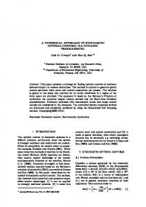
In the framework of fluid dynamics, a special place is taken by free-surface flows. These flows are characterized by the interaction of two or more fluid phases, that do not mix: the interfaces that separate the phases are free to move and deform, and thus they are called free surfaces. This kind of physical phenomena is of major relevance in a large set of applications, both at the large scale, like in the study of water waves and the design of watercraft, and at the microscopic scale, e.g. in the microfluidics of capillary tubes, printing devices or labs-on-a-chip. In many of these applications, a solid wall may be present, and it geometrically restricts the interplay between the fluid phases, giving rise to a contact line, that is the line where the free surface intersects the wall. The leading application described in Sec. 1.1 guided the overall work discussed in the present thesis. In order to highlight the scientific relevance of the present research, it is worthwhile to state since now the mathematical model that we are going to analyze. The geometric settings of the problem are described in Fig. 1.2: the domain there depicted basically reproduces the region near the free surface, inside

1.2 Free-surface problems: state of the art

5

γHν

γ(cos θ − cos θs )

b θ

θ bs

g

τ ∂Γ⊗ b Γ ζ

θ Σ

Fig. 1.2 Geometrical settings of a free-surface problem. the nozzle of the cartridge sketched in Fig. 1.1. The fluid domain Ω is enclosed between the solid wall Σ, the free surface Γ, corresponding to the meniscus of the ink, and the virtual bottom edge Σb , that separates the region of interest of the nozzle from the rest of the fluid. The normal versor is denoted by ν and the unit vector tangential to the contact line ∂Γ is τ ∂Γ . The principal directions of prolongation for the free surface and the wall are identified by b = τ ∂Γ ∧ ν|Γ and bs = ν|Σ ∧ τ ∂Γ ; the contact angle θ between the two surfaces is such that cos θ = b · bs . As already stated above, the main matter pertaining to the simulation of multiphase flows is the description of interfaces between different phases. A whole zoo of models can be found in the literature, in this regard, each one of which was developed to answer to particular needs. Three main categories of models can be identified, depending on how directly they describe the interface. The phase-field model [Sal13, GGM16, NSW14] is representative of the first category: regions occupied by different phases are identified by different integer values of a scalar function, and the interface has a finite thickness, spanning the region where this function smoothly passes from a level to another. This kind of smoothing of the interface allows an accurate physical characterization (including phase transitions) and helps in the development and the proof of theoretical results, but does not provide a sharp position of the interface. On the other hand, in interface-capturing methods, like the level-set method [SSO94, ZGK09] or the volume-of-fluid method [HN81, TSZ11], a precise description of the interface is given at any time, as a codimension-1 manifold immersed in the domain. However, these methods require the solution of both


6

the fluid phases separated by the interface, and at the discrete level it is crucial to properly handle the elements of the computational domain through which the interface passes, since the grid is not conforming to the interface. Eventually, the class of interface-tracking methods includes techniques that track the interface as an actual boundary of the domain, which is thus moved accordingly. The computation of the domain motion is a major point of these techniques, and the Arbitrary Lagrangian-Eulerian approach (ALE) [Don83, FN99] is widely adopted to this aim. Since the interface is not immersed in the domain, in many cases one can actually restrict the computational domain to a single phase of interest. In the present thesis, the ALE approach is adopted, and thus the computational domain we consider is just the domain Ω of Fig. 1.2. In this region, we assume that an incompressible Newtonian fluid is present, so that the following Navier-Stokes equations hold: ∂t u − div ν∇u + ∇uT ) + ∇p = g, div u = 0. On the free surface Γ, surface tension induces the following relation between the normal stress of the fluid and the total curvature H of the surface: ν(∇u + ∇uT )ν + γHν = 0, where γ [m3 /s2 ] is the surface tension coefficient. In addition to this kinetic condition, geometry and fluid velocity are interrelated also by the following kinematic condition u · ν = x˙ · ν,

on Γ,

where x˙ denotes the material velocity of a particle occupying position x ∈ Γ. For many different applications, the overall description of the free surface is not enough, since it is of paramount importance to well describe what happens near the intersection between different interfaces. This intersection, like the line ∂Γ in Fig. 1.2, is called triple line or, when one of the phases involved is a solid, contact line. The physical phenomena occurring at a contact line involve very strong microscopic effects, due to the combination of surface tension and adhesion forces, that can contribute to the occurrence of capillary effects such as the determination of a specific contact angle between the free surface and the wall. These effects, then, can also significantly influence the macroscopic behavior of the physical system, like in the case of capillary action and wicking, or the pinching of droplets on a solid substrate. Despite contact lines are almost ever-present in free-surface flows, modeling their effects without resorting to molecular-scale considerations is still matter of discussion, in the applied mathematical literature. The main hurdle to an accurate

1.2 Free-surface problems: state of the art

7

mathematical description of the fluid motion near the contact line comes from the so-called moving-contact-line paradox. In fact, classical hydrodynamics would suggest to impose no-slip conditions on the wall, as it is very often done in fluid dynamics modeling, i.e. enforcing u=0

on Σ.

However, this imposition would determine a zero velocity of the fluid also at the contact line ∂Γ = Γ ∩ Σ, that would not be able, thus, to slide along the wall, contrarily to the actual motion that everyone can experience by pouring a liquid from a container. To overcome this impasse, different approaches have been proposed in the literature. Early approaches were based on heuristic ideas, e.g. considering the fluid domain Ω to include a thin portion of the space beyond the wall Σ. In this way, ∂Γ happens not to lie on the wall, and then its velocity is allowed to be different from zero. Later approaches began taking into account the contact angle θ. A first idea along this line can be found in [YSS03], where the observation of pinching phenomena is reproduced by introducing some condition on the contact angle: • if θ exceeds some threshold advancing angle θa , and the fluid velocity near ∂Γ is directed upwards, the contact line is advanced upwards; • if θ is lower than some (negative) threshold receding angle θr , and the fluid velocity near ∂Γ is directed downwards, the contact line is moved downwards; • otherwise, ∂Γ remains fixed. Though giving acceptable results in some test cases, this approach is roughly taking into account the physics of the problem, summarizing it in an on/off actuation of the movement. More refined viewpoints consider the region near the contact line separately from the rest of the fluid domain. Local mass and momentum balances are employed to obtain the equations to be set in this microregion, and then appropriate coupling techniques are introduced to connect the local results with the macroscale behavior of the fluid: cf., e.g., [Shi97]. In the last decade, increasing attention has been gained by a boundary condition that looks to be able to introduce quite naturally the dynamics of the contact line in the system equations: the generalized Navier boundary condition (GNBC). Introduced for the first time in [QWS06b], it replaces the no-slip conditions on Σ with the following: u · ν = 0,

ν(∇u + ∇uT )ν − pν + βu · τ = γ(cos θs − cos θ)bs · τ δ∂Γ ,

(1.1)


8

where τ is any vector tangent to Σ and δ∂Γ is the Dirac delta function concentrated on the contact line ∂Γ. Here, the tangential velocity is not set to zero, but it is enforced to depend on the fluid tangential stress and on the uncompensated Young stress - the right-hand side of (1.1). The latter is a force concentrated on the contact line and with an intensity depending on the discrepancy between the current contact angle θ and its static value θs , which is a precise physical property of the system, that can be determined by means of experiments. The validity of the GNBC is assessed also by molecular dynamics simulations [QWS06b] and by physical variational principles [BA11]. Therefore, this boundary condition is adopted also in the present thesis. Most of the mathematical models and techniques hinted above, to appropriately describe the physical system under inspection, present features that require advanced analytical tools and refined numerical techniques. This shows the importance of a scientific research on these topics. As a matter of fact, contact lines are codimension2 manifolds at the boundary of bulk domains, thus highly singular terms can be involved in the mathematical model. An illustrative example of this is the presence of the contact-line delta force in the GNBC, that poses a strong question on the variational settings that should be considered: indeed, the usual Sobolev spaces employed for Navier-Stokes equations do not provide enough regularity to consider the application of a codimension-2 Dirac delta on their elements. Concerning the numerical approximation and the simulation of these problems, the difficulties related to the geometric description of the domain are added to the the abovementioned theoretical issues. A correct reproduction of the physical phenomenon under investigation, in fact, cannot disregard an accurate representation of the geometric quantities involved, and a faithful discretization of the time evolution of the domain and its boundaries.

1.3

Objectives and workflow of the thesis

The present work is guided by the leading application described in Sec. 1.1, and it ultimately aims at designing an optimal control strategy for that system, in order to be able to control the evolution of the free surface and the contact line by acting on other boundary conditions. As displayed in Sec. 1.2, a thorough understanding of the mathematical model under investigation requires to answer questions arising at different levels. In the present section, the workflow of the present research is described, and the main attained objectives are presented. To this aim, some of the mathematical notation of the present thesis is going to be quickly introduced, although rigorous definitions are delayed to the following chapters.

1.3 Objectives and workflow of the thesis

1.3.1

9

Numerical approximation of a free surface problem

Designing a strategy to control the behavior of a physical system and to guide it towards a desired configuration requires, first of all, the knowledge of the phenomenon under inspection. In this regard, a large part of the present work is devoted to the investigation of the flow problem per se. A particular focus is initially given to its numerical simulation, in order to obtain information on the dynamics of the system. Collecting the equations already introduced for the description of the system, we obtain the following differential problem:   ∂t u + (u · ∇)u − div ν(∇u + ∇uT ) + ∇p = g       div u = 0       ν(∇u + ∇uT )ν · τ = 0      T   ν(∇u + ∇u )ν · ν − p + γH = 0 u · ν = x˙ · ν     u·ν =0       (ν(∇u + ∇uT )ν + βu + γ(cos θ − cos θs )δ∂Γ bs ) · τ = 0       u = 0 OR ν(∇u + ∇uT )ν + pν = ζ     u = u0

in Ωt , t > 0, in Ωt , t > 0, on Γt , t > 0, on Γt , t > 0, on Γt , t > 0,

(1.2)

on Σt , t > 0 on Σt , t > 0, on Σb , t > 0, in Ω0 , t = 0,

where τ is any vector tangent to the boundary, and at the lower boundary Σb one can alternatively set a solid wall, on which no issue results from imposing no-slip conditions, or an open boundary with a stress condition. A crucial point in the mathematical modeling and numerical solution of problem (1.2) is to manage the relationship between the physical phenomena governing the evolution of the flow and the geometrical configuration where they take place. In the simulations that will be presented in the next chapters, the ALE approach is employed, to describe the discrete time evolution of the domain. This means that the domain Ω(n+1) at the discrete time step t(n+1) is defined as the image of the domain (n) Ω(n) at the previous time step t(n−1) via the mapping x 7→ x + (t(n+1) − t(n) )Vh , (n) where Vh is the discrete domain velocity, defined as a function on Ω(n) . Thus, the kinematic condition u · ν = x˙ · ν becomes (n)

(n)

uh · ν = V h · ν (n)

on Γ(n) ,

(1.3)

where uh is the discrete fluid velocity. Once the fluid velocity at time t(n) is known, (n) equation (1.3) allows to define Vh by means of a regular lifting (cf. Sec. 2.4.1 and

10


reference [Don83]), so that the next configuration Ω(n+1) is obtained and the time evolution of the solution can be advanced. The strategy just described can be named as explicit treatment of the geometry, since the domain Ω(n+1) is defined in terms of quantities living at the time t(n) , and (n+1) (n+1) the fluid velocity and pressure uh , ph are obtained afterwards, by the solution of the system (1.2) on a known domain. This choice is shared by many other works of the ALE literature, but it is not the only possibility: an implicit treatment of the geometry can be considered, where the domain Ω(n+1) implicitly depends on (n+1) the fluid velocity uh at the same time step, or also multistep techniques can be employed (like, e.g., in [GL09]). The advantage of an implicit choice, w.r.t. an explicit one, is that in general it shows better stability properties of the discrete scheme. However, the cost for this advantage is in terms of computational effort, that can become significantly higher. Though this difference is in accordance with the general behavior of implicit and explicit schemes, it has been mostly observed only by means of simulations, and very few theoretical results are available in the literature, in this regard [GL09]. One of the main results of this thesis is the deep analyses of the numerical scheme resulting from the explicit treatment of the geometry, and the design of a computationally inexpensive stabilization technique to damp out spurious oscillations of the free surface and avoid the need of employing extremely small time steps. Indeed, as observed also in [GL09], the discrete scheme presents some artificial power sources, that can quickly spoil the description of the free surface if an extremely small time step is not chosen. In order to achieve the above-mentioned results, the physical principles underlying the system at hand were analyzed. From them, it was possible to derive the equations (1.2) by variational arguments - thus giving them a physical justification - and write a power balance that shows how the single terms of the equations contribute to the energy of the system. Writing the discrete counterpart of the power balance, spurious terms were identified, and a connection could be observed with the oscillations occurring at the free surface. The origin of this behavior could be found in the statement of the free-surface counterpart of the Geometric Conservation Law, that is in turn a discrete version of Reynolds transport theorem.Analyzing the proof of such a statement, an asymptotically consistent stabilization form could be introduced into the scheme, yielding the improvements hinted above. Concerning the computational effort required by the simulations, although the stabilization of the discrete scheme helps in limiting the number of time steps, one cannot actually consider too large time steps, if accurate results are aimed. This observation makes questions rise about the possibility to reduce the computational


11

burden, that represented the origins of the interest in the reduction technique that will be discussed later on in the present section.

1.3.2

Theoretical analysis of a simplified problem

The simulation of the system solution and the numerical treatment of its peculiarities revealed some interesting features of the equations modeling the phenomenon, such as the presence of singular source terms, the importance of a faithful description of the coupling between the evolution of the geometry and of the fluid inside, the relation between different kind of boundary conditions, and the effects of the imposition of a contact angle. It would, thence, be interesting to inspect these aspects also from a theoretical perspective. However, due to the strong interdependence of all the issues above, the mathematical analysis of the complete fluid-dynamics problem is quite far from being straightforwardly carried out. Anyway, some of the main characteristics of the system under investigation can be found also in simpler differential problem, that are more manageable on the theoretical level. Since the main features that characterize the flow problem (1.2) considered so far are the presence of a free surface and the imposition of the contact angle, we can think of isolating them by considering the following differential problem:      

−∆u = 0 u=g

 ∂ν u = γ H w     ∂ν u = 0

in Ωω

(1.4a)

on Γω ∪ Σb

(1.4b)

on Γω

(1.4c)

on Σω

(1.4d)

where ω : [0, 1] → R is a function whose graph defines Γω : Γω = {(x, y) ∈ R2 : x ∈ (0, 1), y = 1 + ω(x)}, and Ωω is the image of the unit square Ω0 = (0, 1)2 via the transformation (x, y) 7→ (x, y[1 + ω(x)]). The coupling between the solution u of problem (1.4) and the function ω defining the geometry comes from the dynamic condition (1.4c) involving the curvature Hw , that we can write explicitly in term of ω as follows: γ ∂ν u(x, 1 + ω(x)) =

ω ′ (x) p 1 + ω ′ (x)2

!′ .

(1.5)

Considering ∂ν u fixed on Γω , this relation is actually a second-order differential equation for ω, thus we complete it with the imposition of the contact angles at the


12

endpoints of the interval (0, 1): ω ′ (0) = 0,

ω ′ (1) = ψ.

(1.6)

With this observation, the free-boundary problem for the Laplacian can be actually seen as the combination of a problem for u made of (1.4a)-(1.4b)-(1.4d) and one for ω made of (1.5)-(1.6). The mathematical analysis of free-boundary problems is not a new topic in the literature, however, very often, the results that are available have a limited range of applicability, since they generally make large use of the differential operators and boundary conditions defining the problem under inspection. Concerning freeboundary problems for the Laplacian, a milestone contribution is the paper [SS91], where fully Dirichlet boundary conditions are imposed on u, and the position of the contact points is fixed: w(0) = w(1) = 0. In that work, local existence and uniqueness for the pair (u, ω) are proved via a fixed-point argument, together with the stability and convergence of a piecewise linear FE approximation. To the best of the author’s knowledge, few generalizations or extensions of such results have been developed, so far: in [BCCK05] free-surface potential flows are addressed, but no surface tension is accounted for, while [GNS05] extends a crucial instrumental result on Riesz projection to the case of Stokes equations with fully Dirichlet boundary conditions. In this theoretical framework, the present thesis extends the results of [SS91] to the case of the moving-contact-line problem (1.4)-(1.6), for which it is worthwhile to remark that mixed boundary conditions are considered. As stated in [SS91], in fact, this objective is not straightforwardly achievable. To obtain such extension, the variational settings of the differential problem are modified according to the new boundary conditions. Then, the definition of an appropriate lifting operator allows to perform the fixed-point iteration that yields the well-posedness of the problem, at the continuous level. Regarding the analysis of the piecewise linear FEM, optimal stability and convergence could be obtained by proving a stability result for the Riesz projection onto the discrete space, in the case of mixed boundary conditions. A future combination of this result with those of [GNS05] will hopefully help the numerical analysis of the complete flow problem (1.2) guiding the purposes of the present thesis.

1.3.3

Optimal control of free surface problems

After a thorough description and inspection of the flow problem, the field is ready to tackle the optimal control of the physical system outlined in Sec. 1.1. Different


13

aspects of the problem are considered, and the present work addresses both the design of an actual optimization strategy for the industrial application at hand and the investigation of the mathematical issues entailed in the optimal control of a class of free boundary problems. Referring to the guiding application of Sec. 1.1, the optimal control problem we aim at solving has the following form: Find ζ = arg min ∗

ζ∈Mad

Z 0

T

Z

Z

1 jΩ (u) + jΓ (u) + 2 Ωt Γt

Z

subject to   ∂t u + u · ∇u − div σ = g      div u = 0     u · ν = V · ν   σν · ν + γH = 0, σν · τ = 0      u · ν = 0, [σν + βu + γ(cos θ − cos θs )δ∂Γt bs ] · τ = 0     σν = ζ

0

T

Z

|ζ|2 ,

Σb

in Ωt , in Ωt , on Γt , on Γt , ∀τ ⊥ ν on Σt ∀τ ⊥ ν, on Σb ,

where the control function is the time-dependent vector stress ζ living on Σb . In order to tackle this problem, the instantaneous control technique [Hin00] can be employed. The idea of instantaneous control is to split the time interval [0, T ] in a finite number of time slabs [t(n) , t(n+1) ], and to separately consider the contributions of each slab to the total objective functional. Then, the minimization is performed one sub-interval at a time, i.e. solving the following minimization problems, for increasing n: Z Z Z 1 (n+1) (n+1) (n+1) |ζ|2 , Find ζ = arg min jΩ (u )+ jΓ (u )+ 2 (n+1) (n+1) ζ∈Mad Σb Ω Γ subject to u(n+1) solving a discrete step of the problem. For this problem, then, a Lagrangian functional is introduced, and the definition of an adjoint problem allows to derive the gradient of the functional J (n+1) with respect to the control. The interesting point of this approach is that the adjoint problem relative to J (n+1) , albeit depending on the state variables u(n+1) , p(n+1) , is a stationary problem. Therefore, by using instantaneous control one can avoid the mathematical complexity and computational burden of standard optimization techniques that require the solution of the whole time evolution of the state variable to be coupled with a backward-in-time adjoint problem on the whole time interval [0, T ].


14

ν

Γ Σ ω

Ω

ν

Fig. 1.3 External domain Ω of the Bernoulli problem. The final outcome of this scheme is a control function {ζ (n) }N n=1 that is piecewise constant in time. The results that will be presented in the next chapters show that it actually is an effective procedure for the purpose of the present research. Indeed, this control technique allows to reduce significantly the amplitude and the duration of the natural oscillations that can occur in a filling capillary tube. This was exactly one of the main issues of the inkjet printing application described in Sec. 1.1, for which the studies carried on in the present thesis allowed to answer. After having developed an appropriate response to the industrial application motivating the present research, the investigation moves on to a deeper examination of the Lagrangian approach for the optimal control of free boundary problems. To this aim, a simpler class of stationary differential systems has been taken into account: surface tension and the presence of the contact line have been set aside, and the optimal control for the exterior Bernoulli problem [KKL14, LP12] has been addressed. The domain of this problem is depicted in Fig. 1.3: the fluid occupies a region Ω surrounding a fixed domain ω, from which it is separated by Σ = ∂ω; the free boundary enclosing the fluid domain is denoted by Γ = ∂Ω. The state equations constraining the optimization are similar to the (1.4) considered above:  −∆u = f      u=0  ∂ν u = h     ∂ν u = ζ

in Ω(ζ),

(1.7a)

on Γ(ζ),

(1.7b)

on Γ(ζ),

(1.7c)

on Σ,

(1.7d)

where the explicit dependence of the domain on the control variable ζ ∈ Mad is b ⊃ Ω(ζ), ∀ζ ∈ highlighted, and f, h are given functions over an all-holding domain Ω Mad . It has been observed that, for any fixed ζ, the state problem (1.7) can be restated as a shape optimization problem in which one of (1.7b)-(1.7c) is removed from the


15

differential problem and encoded in an objective functional (cf., e.g., [KKL14]). In the present thesis, it is chosen to impose by minimization the Dirichlet condition (1.7b), so that 1 Ω(ζ) = arg min 2 Ω∈O

Z

|u|2 , subject to (1.7a)-(1.7c)-(1.7d),

Γ

where O is the set of admissible domains. With this reformulation, an optimal control problem can actually be seen as a bilevel optimization problem, in the form min J(Ω(ζ), ζ)

ζ∈Mad

subject to Z 1 Ω(ζ) = arg min |u|2 2 Γ Ω∈O subject to (1.7a)-(1.7c)-(1.7d). A bilevel shape optimization problem has been recently studied, for the Bernoulli problem, in [KKL14], and a similar approach has been employed in [LW15] to control the footprint of an inviscid droplet resting on a solid plane, described by equations living only on the its boundaries. In these works, the gradient of the upper level functional J is obtained by means of shape sensitivity equations and direct computation of shape derivatives. This task can get quite tough in the case one wants to extend the results to more complex problems. An alternative approach is represented by Céa’s Lagrangian approach, which exploits the introduction of adjoint differential problems in order to compute the objective functional gradient without the need of a direct computation of the total derivative with respect to the control. Since the present research actually aims at moving towards the control of a complete flow problem, the Lagrangian approach has been adopted: indeed, the interpretation of the adjoint problems helped the design of an optimization algorithm. This different viewpoint allowed the author to abstract from the particular differential problem under investigation, and to design an optimization strategy for a quite general class of bilevel optimization problems with moving geometries. The sufficiently general


16

problem representing this class can be formulated as min J(Ω(ζ), ζ)

ζ∈Mad

subject to (Ω(ζ), u(ζ)) = arg min j(Ω, u) (Ω,u)∈O×V

subject to a(Ω)(u, v) = F (Ω, ζ)(v)

∀v ∈ W,

where {a(Ω) : V × W → R}Ω∈O , {F (Ω, ζ) : W → R}(Ω,ζ)∈O×Mad are families of bilinear and linear forms on the Hilbert spaces V, W , whose elements satisfy the hypotheses of Babuška-Lax-Milgram theorem, and j : O × V → R is the lower-level R objective functional - that is, for the Bernoulli problem above, j(Ω, u) = 12 Γ |u|2 . Employing shape calculus results and finding a novel interpretation of the adjoint variables in terms of the shape derivatives of the state variables, it has been possible to apply the gradient method to the quite general class of optimization problems above. This algorithm was, then, particularized for the Bernoulli problem under consideration, highlighting the role of geometric quantities like the curvature of the free surface.

1.3.4

Reducing the computational effort

As already pointed out, the solution of free-surface flows can be computationally demanding. This load is, then, even more heavy if sensitivity analysis with respect to parameters or the optimal control of these flows is involved, since the direct problem needs to be solved multiple times, for different settings of the mathematical model. In order to take into account also this issue, part of the present thesis is devoted to the design of a reduced order method to pare the computational effort of the solution of a differential problem. Once again, the complexity of the reference problem would strongly limit a deep analysis of the reduction technique applied to it, and thence a simpler differential problem is considered. The parametrized eigenvalue problem for elliptic operators has a sufficient complexity to gain substantial computational savings from the application of the reduced basis method that is employed in this work, particularly due to the presence of a nonlinear interdependence between the solution of the differential problem (the eigenfunction) and another important quantity featured in the problem (the eigenvalue). Studying this problem allows to examine the reduction technique, with its power and limits, while at the same time, a scientific contribution is given, by approaching a problem of interest that has not been comprehensively investigated, yet, in the field of the reduced basis methods.


17

Future developments of the present research may combine the reduced basis method with the methods and algorithms developed in the rest of the present thesis. In fact, some results have been published on the application of the RB method to flow problems, but the knowledge of the particular problem to be reduced always plays a major role in the design of effective reduction techniques. Thence, the broadspectrum investigation conducted in the present work could represent a convenient starting point for the design of a RB method for free-surface problems with moving contact line.

1.3.5

Outline of the thesis

As it can be observed from the discussion conducted in the current section, in the present research, the questions risen by the leading application of Sec. 1.1 are addressed from different viewpoints and with a depth that is correlated with both the complexity of the issues at hand and the mathematical tools that are employed to deal with them. This multi-faceted perspective is mirrored by the structure of the present thesis. Chapter 2 addresses the numerical simulation of a free-surface flow inside a capillary tube. Surface tension, capillary effects and wall friction are taken into account in the equations describing the system, in order to correctly reproduce the dynamics of the contact line. The Finite Element Method is employed, to discretize the spatial domain and the solution of the problem, and the domain evolution in time is described by means of an Arbitrary Lagrangian Eulerian approach. The main contribution of this first part of the thesis is the introduction of a novel stabilization term that can effectively damp the spurious oscillations sprouting from the time-discrete approximation of the domain evolution. This result mainly hinges upon the analysis of the physical principles governing the system under inspection. Numerical tests assess the effectiveness of the approach and the influence of the parameters. A free-boundary problem with moving contact points for the Laplacian operator in two dimensions is tackled in Chapter 3. The free boundary is described as the graph of function, and a contact angle is imposed, at both its ends. The existence and uniqueness of the weak solution of the problem in suitable Sobolev spaces is proved by a fixed-point argument, starting from the inf-sup stability of the variational formulation. Then, a piecewise linear, finite element discretization is introduced, and the stability and convergence properties of the resulting scheme are analyzed. With respect to the present literature, the work carried out in this chapter considers different boundary conditions, both for the geometric and the bulk problem. This is in line with the general interest on applications that characterizes the present


18

thesis: in fact, in real applications it is seldom possible to practically prescribe the position of contact points: moreover, mixed boundary conditions are often more appropriate to describe the interaction between the system under investigation and the environment surrounding it. Some technical, but crucial aspects are then addressed, at both the analytical and the numerical level, such as the definition and regularity of a lifting operator and the stability of the Riesz projection onto the discrete space. In Chapter 4, optimal control problems and optimization procedures are investigated, exploiting the knowledge about the direct problem developed in the previous two chapters. Different strategies are adopted to approach the solution of problems with increasing levels of complexity. In the first part of the chapter, an abstract bilevel optimization algorithm is derived, for the control of differential systems with moving geometries. Then, the control of a stationary free-surface flow is addressed, and the two-level Lagrangian approach is compared to a pseudo-transient formulation of the optimization procedure. Eventually, the optimization of the evolution the full unsteady flow problem described in Chapter 2 is tackled, via instantaneous control. The implementation of this technique allows to effectively contain the naturally oscillatory dynamics of the system, and thus to reduce the overall duration of the transient, as it is shown by numerical tests. The last Chapter 5 concerns the rapid and reliable approximation of parametrized elliptic eigenvalue problems, by means of the Reduced Basis method. Dual weighted residual type a posteriori error estimators are derived, for both the first eigenvalue and the corresponding eigenfunction. Their reliability is proven and they are exploited in a greedy procedure, in order to build up the reduced space. Moreover, they are used also to certify the reduced basis approximation with respect to the high-fidelity one. The computational effectiveness and the overall validity of the proposed approach are displayed by several numerical experiments. On the software To obtain all the simulations and numerical results presented in the present thesis, a significant work was performed by the author on the development of ad hoc software tools. For the rest of the thesis, instead, a C++ software library was developed, in the context of the Aegir project that aims at producing a library to solve PDEs and optimal control problems in the presence of moving domains. This library is based on FEniCS/DOLFIN 2 , which is a solid-base software project, and thus represented a good base onto which developing the utilities required by the applications entailed 2

http://fenicsproject.org

References of the chapter

19

by the present thesis. In particular, the author performed the programming work involving the treatment of moving meshes and the imposition of particular source terms - like the Dirac-delta term on the contact line - that required to extend the features of FEniCS at the level of the structures representing the in-silico counterparts of the variational objects involved in weak formulations and also at the level of the definition and assembling of the algebraic structures required to solve the problem.

References of the chapter [BA11] G. C. Buscaglia and R. F. Ausas. Variational formulations for surface tension, capillarity and wetting. Computer Methods in Applied Mechanics and Engineering, 200(45):3011–3025, 2011. [Don83] J. Donea. Arbitrary Lagrangian Eulerian methods. In Computational Methods for Transient Analysis, V. 1. North-Holland, Elsevier, 1983. [FN99] L. Formaggia and F. Nobile. A stability analysis for the arbitrary Lagrangian-Eulerian formulation with finite elements. East-West Journal of Numerical Mathematics, 7(2):105–131, 1999. [GL09] J.-F. Gerbeau and T. Lelièvre. Generalized Navier boundary condition and geometric conservation law for surface tension. Computer Methods in Applied Mechanics and Engineering, 198(5–8):644 – 656, 2009. [HN81] C. W. Hirt and B. D. Nichols. Volume of fluid (VOF) method for the dynamics of free boundaries. Journal of Computational Physics, 39(1):201– 225, 1981. [LW15] A. Laurain and S. W. Walker. Droplet footprint control. SIAM Journal on Control and Optimization, 53(2):771–799, 2015. [NSW14] R. H. Nochetto, A. J. Salgado, and S. W. Walker. A diffuse interface model for electrowetting with moving contact lines. Mathematical Models and Methods in Applied Sciences, 24:67–111, 2014. [QWS06b] T. Qian, X.-P. Wang, and P. Sheng. A variational approach to moving contact line hydrodynamics. Journal of Fluid Mechanics, 564:333–360, 2006. [Sal13] A. J. Salgado. A diffuse interface fractional time-stepping technique for incompressible two-phase flows with moving contact lines. ESAIM: Mathematical Modelling and Numerical Analysis, 47(3):743–769, 2013.

20

Motivation and workflow of the thesis [Shi97] Y. D. Shikhmurzaev. Moving contact lines in liquid/liquid/solid systems. Journal of Fluid Mechanics, 334:211–249, Mar 1997. [SSO94] M. Sussman, P. Smereka, and S. Osher. A level set approach for computing solutions to incompressible two-phase flow. Journal of Computational Physics, 114(1):146–159, 1994. [TSZ11] G. Tryggvason, R. Scardovelli, and S. Zaleski. Direct numerical simulations of gas–liquid multiphase flows. Cambridge University Press, 2011. [YSS03] J.-D. Yu, S. Sakai, and J. A. Sethian. A coupled level set projection method applied to ink jet simulation. Interfaces Free Boundaries, 5(4):459–482, 2003.

[ZGK09] S. Zahedi, K. Gustavsson, and G. Kreiss. A conservative level set method for contact line dynamics. Journal of Computational Physics, 228(17):6361– 6375, 2009.

Chapter 2 Stability analysis of a moving-contact-line problem We present a free surface problem for time-dependent Navier-Stokes equations is analyzed. Surface tension, capillary effects and wall friction are taken into account in the evolution of the system, influencing the motion of the contact line and of the dynamics of the contact angle. The differential equations governing the phenomenon are first derived from the variational principle of minimum reduced dissipation, and then discretized by means of the ALE approach. The numerical properties of the resulting scheme are investigated, drawing a parallel with the physical properties holding at the continuous level. Some instability issues are addressed in detail, in the case of an explicit treatment of the geometry, and novel additional terms are introduced in the discrete formulation in order to damp the instabilities. Numerical tests assess the suitability of the approach, the influence of the parameters, and the effectiveness of the new stabilizing terms. The results of the present chapter lead to the following work: Ivan Fumagalli, Nicola Parolini, and Marco Verani. On a free-surface problem with moving contact line: from variational principles to stable numerical approximations. Journal of Computational Physics. Under review. MOX preprint 03/2017 available at http://mox.polimi.it/publication-results/?id=649&tipo=add_ qmox.

Stability analysis of a moving-contact-line problem

22

2.1

Introduction

The simulation of free-boundary problems is of major relevance in many fluiddynamics applications, both at the large scale, like in the study of water waves [vdVX07] and the design of watercraft [FMMP08], and at the microscopic scale, e.g. in the microfluidics of capillary tubes [Bos23, YIWK13] or labs-on-a-chip [NSW14, Wal14]. In these settings, the fluid under inspection interacts with other fluids or solids, and thus it is fundamental to correctly track the evolution of the interfaces between the different phases. Different approaches can be found, in the literature, for the modeling and the simulation of multiphase problems, and they can be classified in three main categories, depending on their treatment of the interfaces: the diffuse-interface models, the interface-capturing methods and the interface-tracking techniques. The phase-field model [Sal13, GGM16, NSW14] is representative of the first category: regions occupied by different phases are identified by different integer values of a scalar function, and the interface has a finite thickness, spanning the region where this function smoothly passes from a level to another. This kind of smoothing of the interface allows an accurate physical characterization (including phase transitions) and helps in the development and the proof of theoretical results, but does not provide a sharp position of the interface. On the other hand, in interfacecapturing methods, like the level-set method [SSO94, ZGK09] or the volume-of-fluid method [HN81, TSZ11], a precise description of the interface is given at any time, as a codimension-1 manifold immersed in the domain. However, these methods require the solution of both the fluid phases separated by the interface, and at the discrete level it is crucial to properly handle the elements of the computational domain through which the interface passes, since the grid is not conforming to the interface. Eventually, the third category of methods includes the techniques to track the interface as an actual boundary of the domain, which is thus moved accordingly. The computation of the domain motion is a major point of these techniques, and the Arbitrary Lagrangian-Eulerian approach (ALE) [Don83, FN99] is widely adopted to this aim. Since the interface is not immersed in the domain, in many cases one can actually restrict the computational domain to a single phase of interest. When more than two phases simultaneously interact, particular attention has to be paid to triple lines, where different interfaces intersect. Indeed, the overall evolution of the system is highly influenced by the physical relations occurring on these lines. In case one of the phases under consideration is a solid, the triple line is called the contact line, and if a naïve approach is adopted, one may draw paradoxical conclusions on the physical laws holding thereat. This issue is known as the moving-contact-line problem, and it has been addressed in various ways, in the literature (see, e.g., [GL09, Wal14, Shi97, QWS06a]).

2.1 Introduction

23

In the present work, we analyze a free-surface problem for a Newtonian fluid inside a capillary tube, described by time-dependent, incompressible Navier-Stokes equations and discretized via the Finite Element method (FEM), with an ALE approach accounting for the domain motion. At the free surface, the interaction with a gas is included by means of a surface-tension condition, connecting the curvature of the interface and the stress exchanged between the fluids. The effects of wall friction and contact line forces are gathered in the generalized Navier boundary condition (GNBC), imposed on the solid wall. This condition includes the imposition of an equilibrium contact angle, that is the angle between the free surface and the wall. Such an angle is a primary feature of the shape of capillary menisci and resting droplets, and its imposition by the GNBC has been widely adopted and motivated in the literature of the last decade [GL09, QWS06a, Wal14]. The goal of this work is to investigate the properties of the discretization of the problem under inspection, and to propose a solution to possible stability issues. To this aim, we deeply inspect the structure of the problem, starting from the derivation of the equations at hand from the physical variational principles governing it. This variational approach is shared by other works that can be found in the literature (see, e.g., [BA11, QWS06b, MS09]). Our contribution in this regard is the employment and a mild generalization of the Principle of minimum reduced dissipation [SV12], which represents a general framework for the derivation of differential problems, without resorting to any microscopical consideration. Keeping a parallel between the discrete settings and the laws holding at the continuous level, we will be able to identify the possible sources of instability, in the numerical scheme, and to propose a strategy to control them. This represents a novelty with respect to the results obtained in [GL09]. The present work is organized as follows. In Sec. 2.2, the physical phenomenon under inspection is presented, together with the equations governing it. Domain motion is then addressed, and some shape calculus definitions and results are stated. Then, in Sec. 2.3, the differential problem describing the system is derived from physical variational principles, considering both the case of a closed system, and the possibility of mass exchanges with the environment. Sec. 2.4 is devoted to the weak formulation of the problem and to its ALE-FEM discretization. The numerical properties of the resulting scheme are investigated in Sec. 2.5, in light of the results of Sec. 2.3. Some stability issues are addressed in detail, in the case of an explicit treatment of the geometry, and a novel free-surface stabilization term is introduced. In Sec. 2.6, several tests assess the suitability of the numerical scheme in reproducing the physical phenomena under consideration. Time and space discretization are inspected, and their influence on the physical parameters of the


24

model is examined. Experimental data, taken from [YIWK13], are then employed to validate the numerical scheme. Finally, the effectiveness of the proposed stabilization technique is verified.

2.2

Preliminaries

We consider a fluid contained in a region Ω ⊂ Rd , d = 2, 3, as depicted in Fig. 2.1. The edge Σb is a virtual boundary separating the domain Ω from the rest of the space occupied by the fluid, thus energy and mass exchanges can occur through it. A solid wall is on the lateral side of the domain, and we denote by Σ the part of the wall that is wetted by the fluid at hand, and by Σg the remaining part, in contact with an other fluid, that we assume to be a gas. This gas is separated from the region Ω by the free surface Γ, and we are not interested in studying the gaseous phase, unless for the influence that its presence has on the fluid contained in Ω. The contact line where the three phases meet is denoted by ∂Γ = Γ ∩ Σ. The tangent vector of the line ∂Γ is denoted by τ ∂Γ and we denote by b and bs the unit vectors that are normal to the τ ∂Γ and aligned along the free surface Γ and the wall Σ, respectively (cf. Fig. 2.1, right). On the contact line, we introduce also the function θ : ∂Γ → R denoting the corresponding contact angle, that is such that cos θ = b · bs . The domain at time t is denoted by Ωt and it is identified as the image of an initial domain Ω0 = Ω through a map At : Ω → Rd . A similar notation will be used for all the other quantities, in the rest of the work: the superscript t indicates that the quantity is taken at time t. Assuming the family At of maps to be smooth w.r.t.

Σg

bs

bs

Γ

τ ∂Γ⊗ b

Σ

θ τ ∂Γ

Ω

∂Γ

Σb

Fig. 2.1 Domain and geometric notation. On the right, a zoom near the contact line, in a plane orthogonal to τ ∂Γ .

2.2 Preliminaries

25

time, and each map invertible, we can define the Lagrangian and Eulerian domain velocity fields as b x b) = ∂t At (b V(t, x), ∀b x ∈ Ω, (2.1) t b A−1 (x)), V(t, x) = V(t, ∀x ∈ Ω , t respectively. Being the wall Σt impervious, and wanting to keep Σb fixed, at each time t the domain velocity field V(t, ·) has to belong to the admissible set Uad = v : Ωt → Rd :

v · ν = 0 on Σt ,

v = 0 on Σb .

In the definition above, and throughout the present thesis, by ν we denote the normal vector defined almost everywhere on ∂Ωt . Indeed, for our purposes, we will not need a univocal definition of ν on the zero-measure lines ∂Γt and Σt ∩ Σb . Remark 2.2.1 (Shape kinematics). We point out that the actual evolution of the domain is governed by the sole normal component V · ν of the domain velocity, at the boundary ∂Ωt of the domain. Therefore, any variation of the tangential components or of the bulk distribution, that leaves V · ν unaffected, does not impact on the domain evolution, whence some freedom is left in the definition of V. This freedom will be exploited in the numerical formulation of the free boundary problem. Assuming immiscibility between the different phases involved in the physical system, and neglecting phase transitions, the motion of the free surface Γt follows the movement of the particles of the fluid occupying Ωt . Hence, according to Remark 2.2.1, the geometrical velocity V and the Eulerian velocity u of the fluid are coupled by 1 V·ν =u·ν

on Γt .

(2.2)

Moreover, the fluid in Ωt is assumed to be Newtonian and incompressible, and the forces acting on it are gravity, surface tension, and a possible external stress imposed at the open edge Σb . Hence, supposing to know the initial configuration Ω and fluid velocity field u0 , the state of the flow at time t is described by the current domain Ωt , the fluid Eulerian velocity u and the pressure p. We remark that, thanks to incompressibility, we can consider the rescaled pressure p = pe/ρ, that is the ratio between the physical pressure pe and the fluid density ρ. Analogously, the kinematic viscosity ν = µ/ρ is going to appear in the differential model, in place of the dynamic viscosity µ. The state problem, solved by the couple (u, p) at time t is, then, the 1

For ease of notation, from now on we omit the explicit dependence on time or space, where no misunderstanding is possible.


26

following:   ∂t u + (u · ∇)u − div σ = g       div u = 0        σν · τ = 0, σν · ν + γH = 0

u·ν =V·ν     u · ν = 0, (σν + βu + γ(cos θ − cos θs )δ∂Γ bs ) · τ = 0      σν = ζ     u = u0

in Ωt , t > 0, in Ωt , t > 0, on Γt , t > 0, on Γt , t > 0,

(2.3)

on Σt , t > 0, on Σb , t > 0, in Ω0 , t = 0,

where τ is a generic vector tangent to the boundary, σ = ν ∇u + ∇uT − pI is the stress tensor, I being the identity tensor, g = −ged is the gravity force, ed being the upwards vertical vector of the canonical basis {ei }di=1 , γ is the surface tension coefficient on Γt , H is the total curvature of Γt , β is the friction coefficient on Σt , and ζ is an external stress applied on Σb . The distribution δ∂Γ is defined as Z ⟨δ∂Γ , φ⟩ = φ dλ, for any smooth function φ, ∂Γt

with λ denoting the (d − 2)−dimensional Lebesgue measure on ∂Γt . that the generalized Navier boundary condition (σν + βu + γ(cos θ − cos θs )δ∂Γ bs ) · τ = 0

on Σt

2

We notice

(2.4)

depends both on the current value of the time-dependent contact angle θ and on its static value θs . The latter is defined in terms of the material properties of the three phases interacting around the contact line, through the Young equation [Bat00] γ cos θs + γl − γg = 0,

(2.5)

where γl and γg are the surface tension coefficients on Σt and Σtg , respectively. The discrepancy of the dynamic contact angle θ from θs induces the uncompensated Young stress γ(cos θ − cos θs )τ · bs δ∂Γ , a force which is concentrated on the contact line and oriented along the wall in the normal direction bs to ∂Γt (an upwards vertical force for d = 2). This force is 2

In the rest of the present thesis, Lebesgue measure of any dimension will be understood in all the integrals.

2.2 Preliminaries

27

responsible for the formation of the meniscus in capillary tubes [Bat00], as we will see in the numerical results of Sec. 2.6. The equations (2.3) can be derived from physical principles, in particular employing the Principle of minimum reduced dissipation [SV12]. We are going to devote Sec. 2.3 to this topic, but we want to mention since now that this derivation is prompted by a suitable formulation of the First Law of Thermodynamics, which reads (2.6)

W = 2R, where W is the total power of the external forces, of the form Z Z W= B·u+ T · u, Ωt

∂Ωt

for suitable choices of the generalized forces B = B (g, ρ, pe, u) and T = T(ζ, g, ρ, γ, θs , θ, H, pe), whereas R is the Rayleigh dissipation function, defined as Z Z 1 1 2 e − u · ν ν|2 , 2µ|D(u)| + β|u (2.7) R= 2 Ωt 2 Σt with D(u) = 12 ∇u + ∇uT being the strain rate tensor of the fluid. This law is a fundamental relation governing the physics of the phenomenon, and its discrete counterpart will be explored in Sec. 2.5. In order to actually perform the hinted derivation, we need some technical tools, that we collect hereafter.

2.2.1

Technical tools

In this section, we recall some useful definitions and results that will be employed in the rest of the work. Herein, Γ denotes a generic smooth hypersurface of dimension d − 1, for simplicity immersed in Rd , and ∂Γ indicates its boundary. The tangential gradients of a scalar differentiable function ψ : Γ → R and a vectorial differentiable function ψ : Γ → Rd are defined via the projector ΠΓ = I − ν ⊗ ν: ∇Γ ψ = ΠΓ ∇ψ,

∇Γ ψ = ΠΓ ∇ψ T

T

= ∇ψ ΠΓ .

Accordingly, the tangential divergence of ψ reads div Γ ψ = tr ∇Γ ψ = ΠΓ · ∇ψ. It is possible to prove [DZ11] that the total curvature H of Γ is related to its normal vector ν by div Γ ν = H,


28

whence the following integration by parts formula for surfaces holds [DZ11]: let ψ : Γ → Rd be a differentiable function; then, Z

Z div Γ ψ =

Γ

Z Hν · ψ +

Γ

ψ · b,

(2.8)

∂Γ

where b is the unit vector directed tangentially to Γ and normally to ∂Γ (cf. Fig. 2.1). Since we deal with moving domains, we also recall the Reynolds transport theorem for bulk and boundary integrals: Proposition 2.2.2 (Reynolds transport theorem). Let Γ be a part of the boundary of a domain Ω, and consider two functionals Z Z J1 (Ω) = φ, J2 (Γ) = ψ, Ω

Γ

where φ : Ω → R and ψ : Γ → R are generic differentiable functions. If the domain Ω moves with velocity V, the time derivatives of the functionals read as follows: Z d J1 (Ω) = [∂t φ + div (φV)], dt ZΩ d J2 (Γ) = [∂t ψ + div Γ (ψV)]. dt Γ

(2.9a) (2.9b)

Remark 2.2.3 (Two dimensional case). For d = 2, the contact line ∂Γ is actually the union of two points, and b is the tangential direction prolonging the free surface Γ. The vector bs is aligned to the wall Σ (thus simply vertical, in our case), and there is no need to define τ ∂Γ .

2.3

Derivation of the differential problem from variational principles

The present section is devoted to the derivation of the system of equations (2.3) from physical variational principles. To ease the presentation, we split the derivation into two steps: at first (Sec. 2.3.1), we will consider Σb as an impervious wall (see Fig. 2.1), and subsequently (Sec. 2.3.2), mass exchange will be allowed through this boundary. It is worth remarking that the result in Sec. 2.3.1 has an autonomous interest, e.g. in case droplets on a substrate or sloshing fluid in a tank are regarded [LW15, GL09]. Throughout the present section, we assume sufficient regularity of the functions involved so that the expressions and forms defined below make sense.

2.3 Derivation of the differential problem from variational principles

2.3.1

29

Step 1: derivation in the case without mass exchange

The kinematic conditions require the motion of the free surface Γt to be prescribed by the Eulerian velocity u (cf. (2.2)). Moreover, Σb is a closed boundary, for this first step, thus we do not make any distinction between the fluid velocity and the domain velocity, namely we consider V = u everywhere in Ω. Therefore, the kinematic constraints directly apply on u, that is, for any time t, u belongs to Uad =

u : Ω → R : u · ν = 0 on Σ , u = 0 on Σb , t

d

t

[(∂t ρ + div (ρu)] = 0 ,

Z Ωt

where ρ : Ωt → R is the mass density function. In the definition of the set of admissible velocities we included also the conservation of mass, which can be rephrased locally as in Ωt ,

ρ˙ + ρ div u = 0

(2.10)

with the usual notation ρ˙ = ∂t ρ + u · ∇ρ for the Lagrangian derivative. Regarding dynamics, we assume that only gravity and surface tension act on the system. Being such forces conservative, the system possesses a potential energy Z V=−

Z ρg · x +

Ωt

Z γ+

Γt

Z γl +

Σt

γg ,

(2.11)

Σtg

where the last three terms take into account the pairwise interactions between the fluid in Ωt , the gas above and the solid wall. In the following, we denote by | · | the measure of a set. Combining Prop. 2.2.2 with (2.5),(2.8) and (2.10), and since γ and g are constant and Σt and Σtg are flat, the active power that the environment transfers to the system can be written as Z d d ˙ Wa = −V = ρg · u + γ |Γt | + (γl − γg ) |Σt | dt dt t ZΩ Z Z = ρg · u − γHν · u − [γu · b + (γl − γg )u · bs ] t t t Ω Γ ∂Γ Z Z Z ρg · u − γHν · u − γ(cos θ − cos θs )u · bs , = Ωt

Γt

∂Γt

where in the last line we employed the decomposition u = (u·ν|Σt )ν|Σt +(u·τ ∂Γ )τ ∂Γ + (u · bs )bs on ∂Γt and the identities u · ν|Σt = τ ∂Γ · bs = 0 and b · bs = cos θ. The power transfer Wa affects different forms of energy of the system. A part of it determines an increase in the kinetic energy K of the fluid Z 1 K= ρ|u|2 , 2 Ωt


30

another part is stored as free energy F with mass-specific density ψ = ψ(ρ), just depending on ρ [SV12], Z F= ρψ, Ωt

and, since the fluid is not perfect, a part of this energy is dissipated, resulting in ˙ The connection between the quantities defined above is a entropy production S. given by the First Law of Thermodynamics that, in the case of adiabatic, isothermal transformations, reads ˙ T S˙ = Wa − K˙ − F. (2.12) In this identity, the left-hand side D = T S˙ is called the total dissipation function, ˙ F˙ (called total power in [SV12]) represents whereas the right-hand side W = Wa − K− the amount of power that the system receives and does not transform in kinetic or free energy. From the Second Law of Thermodynamics, we know that it has to hold D ≥ 0, but in order to give this dissipation an explicit expression, we need to introduce a suitable constitutive relation. For the system described in Sec. 2.2, it is quite natural to assume that the only sources of dissipation are friction on the wall Σt and viscosity inside the fluid, thus we can give a constitutive relation for D in terms of the following Rayleigh dissipation function: Z Z 1 1 2 e Σ u|2 , µ|D(u)| + β|Π R= 2 Ωt 2 Σt by setting D = 2R. Now, in order to write the First Law (2.12), we need an explicit expression of the total power W. In particular, we are going to show that it has the following form: Z W=

Z B·u+

Ωt

(2.13)

T · u, ∂Ωt \Σb

where B : Ωt → Rd and T : ∂Ωt \ Σb → Rd are suitably defined generalized forces. The expressions for these two quantities can be retrieved by computing the time derivatives of the kinetic and free energies, and employing the definition of W. Indeed, using the equation of conservation of mass (2.10) and Reynolds transport theorem (2.9a), one can find that K˙ =

Z ˙ ρu · u, Ωt

F˙ =

Z Ωt

ρψ˙ =

Z

′

Z

ρψ ρ˙ = − Ωt

Ωt

ρ2 ψ ′ div u.


31

Concerning the free energy, it is commonly accepted (see, e.g., [SV12]) that pressure is related to the derivative of the free energy density as pe = ρ2 ψ ′ . Thence, after integration by parts of the pressure term, the expression (2.13) of the total power W can be written in terms of the generalized forces    p − γH)ν on Γt ,  (e B = ρg − ρu˙ − ∇e p,

T=

peν    −γ(cos θ − cos θs )bs

on Σt ,

on ∂Γt .

At this point, we have all the ingredients to formulate a variational principle from which to derive the equations of the motion for our physical system: Principle of minimum constrained dissipation. [SV12, p.119] 3 For a deformable body undergoing a process with total power W and Rayleigh dissipation function R, that obeys the Second Law of Thermodynamics in the form D ≥ 0, with D = 2R, the true evolution u at time t is such that R attains its minimum w.r.t. all b = u + δu, once W and the generalized forces B, T are held virtual process rates u fixed. From the formulation of this principle, we see that one should take into account the constraint of holding both W and the generalized forces fixed, while varying the velocity field by a term δu. In order to do this, it is useful to rewrite the principle in terms of a reduced dissipation functional. Following the ideas in [SV12], we can introduce the Lagrangian functional L = R + λW, where λ is the Lagrange multiplier for the imposition of the constraint over W, during the minimization of R. Aiming at enforcing the variations of L to be equal to zero, we compute the variations of R and W induced by a virtual velocity variation δu. Concerning the Rayleigh dissipation functional, it is enough to compute the Gâteaux derivative Z Z δR = ∂u R[δu] = 2µD(u) · D(δu) + βe ΠΣ u · ΠΣ δu. Ωt 3

Σt

In the present work, we are adopting the viewpoint of Continuum Mechanics, thus we talk about minimum dissipation. In the literature of Statistical Mechanics, this principle is looked at as a maximum principle. However, for the purposes of the present work, only the stationarity of the functional is considered, hence we avoid digging any further into this distinction.

32


Dealing with the total power, the Principle requires to hold B and T fixed. Therefore, instead of using the classical Gâteaux derivative, we define the variation of W as Z Z δW = B · δu + T · δu. Ωt

∂Ωt \Σb

Remark 2.3.1. In [BA11, MS09], the constraint on the constantness of the generalized forces B, T is replaced by the requirement that the variations δu are time independent. However, in our approach such a requirement is not admissible. Indeed, the variations δu are actually test functions for the problem, and the ALE approach that will be introduced in Sec. 2.4.1 will require the test function to have zero ALE derivative, thus they cannot actually be time independent. Now we can compute the variations of the Lagrangian functional L induced by δu: 0 = δL = δR + λδW = (∂u R + λδu W) [δu],

∀δu,

where we have introduced the linear functional δu W : δu 7→ δW, with δW defined as above. Now, the value of the Lagrange multiplier λ can be found by imposing the validity of the First Law of Thermodynamics (2.12), which can be rewritten as 2R = D = W.

(2.14)

Indeed, since ∂u R[u] = 2R and δu W[u] = W, combining (2.14) with (∂u R + λδu W)[u] = 0 yields λ = −1. Therefore, the principle of minimum constrained dissipation can be equivalently formulated as follows: Principle of minimum reduced dissipation. [SV12, p.137] For a deformable body undergoing a process with total power W and Rayleigh dissipation function R, that obeys the Second Law of Thermodynamics in the form D ≥ 0, with D = 2R, the true e = R − W attains evolution u at time t is such that the reduced dissipation function R b = u + δu, once the generalized forces its minimum w.r.t. all virtual process rates u B, T are held fixed. That is, the true evolution is characterized by the requirement that δR = δW in any subregion ω ⊆ Ωt , R R where δR = ∂u R[δu], δW = Ωt B · δu + Γt T · δu.

(2.15)

Now we can apply this principle in our settings, in order to obtain the differential equations governing the physical phenomenon at hand. We also assume that the fluid in Ωt is incompressible, hence we can divide both sides of (2.15) by the constant


33

density ρ, without losing generality. 4 Thus, rephrasing the optimality condition (2.15) and writing explicitly the total derivative dtd u = ∂t u + u · ∇u yield Z ω

Z 2νD(u) · D(δu) + β ΠΣ u · ΠΣ δu t ∂ω∩Σ Z = − [(∂t u + u · ∇u − g) · δu − p div δu] ωZ Z − γHδu · ν − γ(cos θ − cos θs )δu · bs , ∂ω∩Γt

∂ω∩∂Γt

e where β = β/ρ. Integrating by parts and using the kinematic conditions u · ν = 0 t on Σ , δu = 0 on Σb , we obtain Z ω

(∂t u + u · ∇u − div (2νD(u)) + ∇p − g) · δu Z + (γHν + 2νD(u)ν − pν) · δu t Z∂ω∩Γ + γ(cos θ − cos θs )δu · bs t ∂ω∩∂Γ Z + ΠΣ (βu − 2νD(u)ν + pν) · ΠΣ δu = 0.

(2.16)

∂ω∩Σt

Since δu is arbitrary, as well as the subregion ω, from (2.16) we can derive the strong formulation of the Navier-Stokes equations with moving contact line. Such equations, combined with the kinematic condition V · ν = u · ν on ∂Ωt (see Remark 2.2.1) and the constraint V · ν = 0 on Σt (see Uad in Sec. 2.2), make up the following differential problem:   ∂t u + (u · ∇)u − div σ = g        div u = 0 V·ν =u·ν     σν · τ = 0, σν · ν + γH = 0      u · ν = 0, (σν + βu + γ(cos θ − cos θs )δ∂Γ bs ) · τ = 0

in Ωt , in Ωt , on Γt on Γt , ∀τ ⊥ ν, on Σt , ∀τ ⊥ ν,

where σ = 2νD(u) − pI is the stress tensor. This problem is well defined for the whole time evolution as soon as we know the initial condition u(t = 0) = u0 . Before passing to the second step of our derivation, we point out that, in the incompressible case, the introduction of the free energy F occurs to be just instru4

Keeping the density ρ explicit until the very end helped in keeping the presentation general and relatively simple. If we had imposed the uniformity of ρ since the beginning, no free energy F would have appeared, and the rescaled pressure p would have needed to be introduced as a Lagrange multiplier for the incompressibility constraint, rather complicating the argument.


34

mental to take into account the pressure p in the equations (this will be true also in the next section). This is the reason why we will not introduce a discrete free energy, in Sec. 2.5.

2.3.2

Step 2: allowing mass exchanges with the environment

So far, we have considered a closed physical system, in terms of mass exchange. However, taking into account the possibility of having an inflow/outflow boundary is a necessity when modeling many phenomena. In this section, we allow the fluid to pass through the boundary Σb (see Fig. 2.1). This part of the domain boundary is going to be fixed in the domain evolution, but in order to flow through it, the fluid may have a nonzero normal velocity u · ν at Σb . Moreover, we account for a possible external surface load ζ, acting on the open boundary. In these new settings, we need to perform some modifications on the definition of the energetic quantities managed above, and on their relationships. First of all, since our domain is not moving in a Lagrangian way together with the particles it contains, the time variation of the physical quantities are not given anymore by their Lagrangian derivative along the fluid velocity u. Therefore, we introduce a different notation for the total derivative along the domain velocity field V: for a scalar field like density we write Dt ρ = ∂t ρ + V · ∇ρ. A similar notation is going to be used for integral quantities, like the free energy: the application of Prop. 2.2.2 yields Z Dt F = [∂t (ρψ) + div (ρψV)] . Ωt

According to this definition for the time derivative, the active power Wa , including also the contribution due to the external surface stress, is now of the form Z Wa = −Dt V + ζ · u. Ωt

Eventually, the total power has to include also the energy flux associated with the mass flowing through the open boundary Σb , whence it has to be re-defined as Z W = −Dt V − Dt K − Dt F +

Z ζ·u−

Ωt

Σb

1 2 ρ|u| − g · x + ρψ u · ν. 2

(2.17)

Having these new definitions, we can perform all the steps followed in Sec. 2.3.1, up to formally writing the principle of minimum reduced dissipation (2.15). The last


35

ingredient we need, in order to obtain the differential equation ruling the physical phenomenon at hand, is the definition of the generalized forces B, T. To this aim, we need to write explicitly all the quantities appearing in (2.17). For the sake of brevity, let us compute explicitly only the total time derivative of the kinetic energy: Z Dt K = Ωt

1 1 2 2 |u| (∂t ρ + V · ∇ρ + ρdiv V) + ρu · ∂t ρ + ρV · ∇|u| . 2 2

˙ we can Noticing that if V = u we would have the Lagrangian time derivative K, write the expression above in terms of K˙ itself, as follows: Z

1 1 1 2 2 2 Dt K = K˙ + |u| (V − u) · ∇ρ + ρ(V − u) · ∇|u| + ρ|u| div (V − u) 2 2 Ωt 2 Z Z 1 1 ρ|u|2 (V − u) = K˙ + ρ|u|2 (V − u) · ν = K˙ + div 2 2 t Σb ZΩ 1 = K˙ − ρ|u|2 u · ν, 2 Σb where we have used that V ·ν = u·ν on Γt ∪Σt . As we can see, the difference between the total derivative of the kinetic energy contained in Ωt and its Lagrangian derivative is given by the opposite of the exiting flux through Σb . Analogous computations for the potential energy and the free energy lead to similar results, thence the total power can be written also as Z ˙ ˙ ˙ W = −V − K − F + ζ · u, Ωt

where the flux terms have been canceled out in the transition from Dt to the derivative ˙ Therefore, the generalized forces B, T read as follows: (·).

B = ρg − ρu˙ − ∇e p,

T=

  (e p − γH)ν     peν

on Γt ,

  peν + ζ     −γ(cos θ − cos θs )bs

on Σb ,

on Σt , on ∂Γt .

Using these expressions, and assuming incompressibility and a homogeneous fluid density, we can employ the Principle of minimum reduced dissipation and eventually obtain system (2.3). Remark 2.3.2. For the sake of clarity we remark that, although the final steps of the derivation formally employ the Lagrangian derivatives of the energies along u, a physically consistent formulation of the First Law of Thermodynamics for the

36


domain Ωt considered here can be written only in terms of the material derivatives along V: this is why the correct definition of the total power is actually (2.17). Remark 2.3.3. In the applied mathematical literature, a variational principle named after Onsager has recently gained some popularity, in the derivation of differential problems [GGM16, NSW14, QWS06b, Wal14]. The formulation of this principle is quite similar to identity (2.15), but its justification is ascribed to Onsager-Casimir reciprocal relations [Ons31a, Ons31b], a principle holding at the microscopic level, whereas the Principle of minimum reduced dissipation is purely macroscopic. As pointed out in [SV12, from p.149], connecting the microscopic reciprocal relations to the macroscopic principle used in the above-mentioned literature is not easy: “Though no objection could be raised against the reversibility of microscopic motions, its reverberations on a macroscopic scale are invariably the object of an assumption, in one fashion or another”. Therefore, in the present work we decided to adopt the procedure developed in [SV12], in the frameworks of Analytic and Continuum Mechanics, avoiding the need of microscopical considerations. This choice gave us a general workflow that could be used to treat both the closed-system case (Sec. 2.3.1) and the case with mass exchange (Sec. 2.3.2). In this regard, it is worth pointing out that the latter case was not considered in [SV12].

2.4

Discretization of the problem

After the introduction and justification of the system (2.3), now we address its numerical solution, and thence we introduce its discretization via the Finite Element Method (FEM). As usual, we first reformulate the system in a suitable weak form, taking into account the domain motion. For the first part of this section, the domain velocity V will be considered as known: the actual coupling of the physical and the geometrical problem will be dealt with in Sec. 2.4.4.

2.4.1

Eulerian and ALE weak formulation

The state of the fluid at hand is represented by its static pressure p and its Eulerian velocity u. In order to comply the kinematic condition on the wall Σt , we introduce the following velocity and pressure spaces: Ve t = {v ∈ [H 1 (Ωt ) ∩ H 1 (Γt )]d : v · ν = 0 on Σt }, Pet = L2 (Ωt ), in which further regularity is required on Γt , to ensure that the forms introduced in the following make sense. Testing problem (2.3) against some (v, π) ∈ Ve t × Pet , we can

2.4 Discretization of the problem

37

formally write the following weak formulation of the problem: given u(t = 0) = u0 , find (u, p) such that for all t > 0 (∂t u, v) + a(u, v) + b(v, p) + c(u, u, v) = F (v) ∀v ∈ Ve t , b(u, π) = 0 ∀π ∈ Pet ,

(2.18)

where (·, ·) is the L2 inner product on Ωt , ν Z T T βu · v, a(u, v) = (∇u + ∇u ), ∇v + ∇v + 2 Σt b(v, π) = −(div v, π), c(w, u, v) = ((w · ∇)u, v), Z Z Z γdiv Γ v + F (v) = (g, v) + ζ·v− Γt

Σb

γv · bs cos θs .

∂Γt

Remark 2.4.1. To obtain formulation (2.18), the Gauss formula (2.8) and suitable geometrical arguments are employed, on the same line as in [GL09]. In particular, focusing on the boundary conditions of (2.3) holding on Γt and Σt , and noticing from Fig. 2.1 that b · bs = cos θ, the following identities hold: Z

Z σν · v = −

(2.8)

Z

Z

γHν · v = − γdiv Γ v + γv · b t t Γ ∂Γ Z =− γdiv Γ v + γ cos θ v · bs t t Γ ∂Γ Z Z Z σν · v = − βu · τ v · τ − γ(cos θ − cos θs )bs · τ v · τ t ∂Γt Σt ZΣ Z =− βu · v − γ(cos θ − cos θs )v · bs , Γt

t ZΓ

Σt

(2.19a)

(2.19b)

∂Γt

where we have also exploited the additional H 1 -regularity on Γt introduced in Ve t , and the fact that v·ν = 0 on Σt , and thus also on ∂Γt thanks to trace theory. Summing up (2.19a) and (2.19b), the terms depending on θ cancel out. Then, standard techniques can be employed to obtain the weak formulation (2.18) [QV94, Tem77]. It is worth to point out that neither the curvature H nor the dynamic contact angle θ appears in (2.18): this significantly simplifies the numerical treatment of the equations, since the explicit discrete approximation of contact angle and curvature requires extra effort and a more sophisticated approach (cf., for example, [MS09, BNP10]). Problem (2.18) is written in Eulerian coordinates, and at a fixed time t. In a numerical discretization, this would imply either keeping the mesh fixed during the time evolution – at the cost of introducing extra theoretical difficulty to deal


38

with the domain movement – or generating a completely new mesh at each time step – thus bringing in a very high computational cost. A widely used technique to have a computationally rather inexpensive mesh motion is to set the equations in an Arbitrary Lagrangian-Eulerian (ALE) framework [Don83, FN99], in which the domain velocity V, defined in (2.1) is considered separately from the fluid velocity u. Associated to the domain velocity, we can define the so called ALE derivative operator, which computes the time derivative of a function φ : Ωt → R along the domain trajectory described by V: ∂tALE φ = ∂t φ + V · ∇φ. It is worth pointing out that the domain velocity V occurs to be the ALE derivative of the position, i.e. V = ∂tALE x. Employing the definition of ∂tALE , problem (2.18) can be formulated in the ALE framework as follows [Don83, GL09]: (∂tALE u, v) + a(u, v) + b(v, p) + cALE (u, V, u, v) = F (v) ∀v ∈ V t , b(u, π) = 0

∀π ∈ P t ,

(2.20)

u(t = 0) = u0 , where b(A−1 V t = {v : Ωt → Rd : ∃b v ∈ Ve 0 , v(x) = v t (x))}, P t = {π : Ωt → R : ∃b π ∈ Pe0 , π(x) = π b(A−1 t (x))}, Z Z cALE (z, V, u, v) = [(z − V) · ∇] u · v − div (V)u · v. Ωt

2.4.2

Ωt

Time discretization

In this section, we discretize the ALE formulation (2.20) w.r.t. time, using a uniform T time discretization made of time steps t(n) = n∆t, n = 0, 1, . . . , N = ∆t . Such a semi-discretization also involves the domain motion, thus we need to discretize the ALE map, introducing the application An,n+1 : Ω(n) → Ω(n+1) ,

An,n+1 (x) = x + ∆t V(n) (x),

where the superscript (n) indicates the time step t(n) at which the quantity is taken (e.g. V(n) (x) = V(t(n) , x)): this notation will be used for all the other quantities involved in the problem. The discretization of the ALE map directly induces the definition of a discrete sequence of domains Ω(n) = An−1,n (Ω(n−1) ), on which the


39

following spaces are recursively defined as V (n) = {v ∈ [H 1 (Ω(n) ) ∩ H 1 (Γ(n) )]d : v ◦ An−1,n ∈ V (n−1) }, P (n) = {p : p ◦ An−1,n ∈ P (n−1) },

(2.21)

where V (0) , P (0) are assigned. Thus one reduces to building up a basis only for the initial spaces V (0) and P (0) , the bases for V (n) and P (n) being obtained via the maps Ai−1,i , i = 1, . . . , n. This represents a remarkable computational saving in the numerical solution of the problem. It is worth noticing that having each V(n) to belong to Uad , the kinematic constraints are preserved, and at each time t(n) the spaces actually correspond to the usual definition, i.e. V (n) = {v ∈ [H 1 (Ω(n) ) ∩ H 1 (Γ(n) )]d : v · ν = 0 on Σ(n) }, P (n) = L2 (Ω(n) ). In view of the above discussion, the time-discretization of problem (2.3) reads as follows: given u(0) , for each n = 0, . . . , N − 1, find (u(n+1) , p(n+1) ) ∈ V (n+1) × P (n+1) such that, ∀(v, π) ∈ V (n) × P (n) , 1 (n+1) (u , v)Ω(n+1) + a(n+1) (u(n+1) , v) + b(n+1) (v, p(n+1) ) ∆t (n+1) +cALE (u(n) , V(n) , u(n+1) , v) + s(n+1) (V(n) , u(n) , u(n+1) , v) 1 (n) = (u , v)Ω(n) + F (n+1) (v), ∆t b(n+1) (u(n+1) , π) = 0,

(2.22)

where the superscript (n) in the spaces and forms indicates that the domain under consideration is Ω(n) . The additional form s(n+1) (·, ·, ·) artificially adds the following strongly consistent stabilization terms: s

(n+1)

(V

(n)

,u

(n)

(n+1)

,u

1 , v) = 2

Z

div (u(n) )u(n+1) · v

Ω(n+1)

1 − 2

(2.23)

Z (u

(n)

−V

(n)

)·νu

(n+1)

· v,

Γ(n+1)

whose presence is widely accepted in the ALE literature [Tem77, GLB03] and whose role will be clear from the proof of Thm. 2.5.1, in Sec. 2.5. Remark 2.4.2. In the terms involved in (4.3), the domain of integration does not always coincide with the domain of definition of the integrands, e.g. v is defined on Ω(n) , but it appears in integrals over Ω(n+1) = An,n+1 (Ω(n) ). In order to keep a


40

light notation, a change of variables via ALE mapping is understood in case this R R discordance occurs: e.g. Ω(n+1) v actually means Ω(n+1) v ◦ A−1 n,n+1 .

2.4.3

The fully discrete problem

In this section, we introduce the space discretization for the problem under inspection. (0) To this aim, let Th be a regular triangulation [Cia78] of the initial domain Ω(0) , with characteristic discretization step h. The triangulation of Ω(n) isobtained through (n) (n−1) repeated applications of the discrete ALE map, i.e. Th = An−1,n Th . In these settings, we can write the FEM approximation of problem (4.3) as follows: given the (0) FEM interpolation uh of the initial velocity field u(0) , for each n = 0, . . . , N − 1, (n+1) (n+1) (n+1) (n+1) (n) (n) find (uh , ph ) ∈ Vh × Ph such that, ∀(vh , πh ) ∈ Vh × Ph , 1 (n+1) (n+1) , vh )Ω(n+1) + a(n+1) (uh , vh ) (uh ∆t (n+1) (n+1) + b(n+1) (vh , ph ) − b(n+1) (uh , πh ) (n+1)

(n)

(n)

(n+1)

(n)

(n)

(n+1)

, vh ) + s(n+1) (Vh , uh , uh + cALE (uh , Vh , uh 1 (n) = (u , vh )Ω(n) + F (n+1) (vh ), ∆t h where

(0)

(0)

, vh )

(2.24)

r

= V (0) ∩ [Xhru (Ω)]d , Ph = P (0) ∩ Xhp (Ω), n o (0) Xhr (Ω) = φ ∈ C 0 Ω : φ|K ∈ Pr (K) ∀K ∈ Th , Vh

(n)

(n)

and Vh , Ph are recursively defined in the same way as in (2.21). In this discrete framework, the friction coefficient appearing in the form a will be denoted by βh : indeed, in Sec. 2.6.2 we will see that a dependence of this coefficient on the mesh size is required, in order to comply experimental data. Remark 2.4.3 (Variational crime). Here we do not make a distinction between the evolution of the domain according to the continuous map At and the sequence of discrete maps An−1,n . This is related to the well-known (and usually disregarded) variational crime [BS07]. In the formulation (2.24), the polynomial degrees ru , rp still need to be chosen. In the present work, we focus on the P1 − P1 pair, namely the case ru = rp = 1: a comment on this choice will be made after the introduction of the problem for the domain velocity V(n) , at the end of Sec. 2.4.4. Hence, in order to cope with the lack of validity of the LBB condition (cf. [GR12, Tem77]), we employ the classical Brezzi-Pitkäranta pressure stabilization [BP84], replacing the ALE stabilization form


41

s(n+1) in problem (2.24) with the form (n)

(n)

(n+1)

s(n+1) (Vh , uh , uh p

(n+1)

, vh , ph

(n)

(n)

(n+1)

, πh ) = s(n+1) (Vh , uh , uh , vh ) Z X (n+1) + Cs h2 ∇ph · ∇πh . (n)

K∈Th

(2.25)

K

So far we assumed the knowledge of the domain velocity V. However, this is part of the unknowns and the following section addresses the construction of the (discrete) geometrical velocity V(n) , which allows to pass from Ω(n) to Ω(n+1) .

2.4.4

Kinematic conditions

As anticipated in Sec. 2.2, the domain velocity V has to undergo some kinematic conditions, in order to ensure a physically consistent evolution of the domain. In particular, being Σt a solid wall, and as the motion of the fluid particles follows the free boundary Γt , the domain velocity must satisfy V·ν =0

on Σt ,

(2.26a)

V·ν =u·ν

on Γt ,

(2.26b)

at any time t. Moreover, since Σb is held fixed, we also require V · ν = 0 on Σb . In view of the discussion in Remark 2.2.1, these conditions are sufficient to determine the overall evolution of the domain Ωt . Therefore, we require the same conditions for (n) the discrete domain velocity Vh . (n) We remark that, since Vh is used to move the mesh, we need an explicit knowledge of all its components at the whole set of mesh nodes. However, conditions like (2.26) prescribe only one degree of freedom of the boundary distribution of such (n) velocity. Hence, we can fix all the other degrees of freedom by requiring Vh to (n) (n) be vertical, namely Vh = vh ed . This yields some useful properties, that will be displayed in Prop. 2.5.2. Then, to determine the bulk distribution of the velocity, we consider a harmonic lifting, which is a widely adopted choice in the ALE literature [BF09, BPS13, GL09] since it generates a regular velocity field, whence the mapped mesh preserves a certain degree of regularity. (n) (n) (n+1) Summarizing, the domain velocity Vh mapping Th to Th can be defined (n) as the solution of the following problem: prescribing Vh to be vertical, namely


42

(n)

(n)

(n)

Vh = vh ed , find vh ∈ Xh1 (Ω(n) ) such that  (n)  ∆vh = 0    v (n) = 0

in Ω(n) ,

(n)   ∂ν vh = 0     (n) vh νd = u∗h · ν

on Σ(n) ,

on Σb ,

h

(2.27)

on Γ(n) ,

where u∗h : Γ(n) → Rd is some discrete counterpart of the fluid velocity u. Different definitions can be given for u∗h , and they have a nonnegligible effect on the stability of the numerical scheme as a whole (cf. Sec. 2.5). In our numerical tests, we adopt the simplest choice for such a velocity, that is, we set (n)

u∗h = uh ,

(2.28)

which corresponds to an explicit treatment of the geometry. In the next section we will analyze its impact on the scheme, and propose an original strategy to cure possible instabilities associated to it. Another possibility, that is also considered in Sec. 2.5, is the implicit treatment of the geometry, determined by (n+1)

u∗h = uh

◦ An,n+1 .

(2.29)

This choice, however, introduces a high nonlinearity in the system, due to the strong coupling between the physical problem (2.20) and the geometrical problem (4.4). Thus, some nonlinear solver is required, and the computational effort is much higher than in the explicit case. This may represent a serious obstruction in case the state problem needs to be solved many times for different parameter values (e.g., in optimal control problems). Other choices for u∗h can be straightforwardly introduced in the scheme, like the extrapolation proposed in [GL09]: u∗h = 2u(n) − u(n−1) ◦ A−1 n−1,n , which benefits from the inexpensiveness of the explicit treatment and, in the numerical test cases considered in [GL09], does not show stability issues. However, up to the authors’ knowledge, no theoretical results are known on the stability of the scheme characterized by this extrapolation. Concluding this section, we comment on some implementation aspects. The choice of piecewise linear elements for the fluid velocity was made in order to ease

2.5 Stability and discrete minimum dissipation principle

43

the implementation, by avoiding curvilinear elements and thus isoparametric finite (n) elements. Eventually, we remark that the actual kinematic condition vh νd = u∗h · ν is imposed in a weak sense, by penalization. In this way, we just need the normal vector ν to be defined on the faces (edges for d = 2) of the boundary, and not on the vertices of the mesh, where it is not univocally determined.

2.5

Stability and discrete minimum dissipation principle

In this section, we want to analyze the properties of the numerical scheme introduced above. In particular, we investigate how the discrete formulation (2.24) can reproduce, mutatis mutandis, the First Law of Thermodynamics (2.12). This will give us information about the stability of our numerical scheme and it will shed light on the critical terms of the discrete formulation, that may give rise to numerical instabilities. On this concern, Sec. 2.5.1 will be devoted to the introduction of a novel free-surface stabilization term, named SΓ , to cure the onset of spurious instabilities. Unlike the forms s, sp defined in (2.23)-(2.25), which involve the well-established stabilization terms required by the ALE approach and the choice of the P1 − P1 finite element pair, the additional form SΓ that is going to be defined represents an original contribution of the present work. Aiming at writing the discrete counterpart of the power balance (2.6), with the total power W and the Rayleigh dissipation function R defined as in (2.17) and (2.7), respectively, we need to introduce some discrete energetic quantities that will take part in the equation. We define the following quantities: 5 R R R R Potential energy V (n) = − Ω(n) g · x + Γ(n) γ + Σ(n) γl + Σ(n) γg , g Kinetic energy K(n) =

1 2

R

|u(n) |2 , R R = 21 Ω(n) 2ν|D(u(n) )|2 + 21 Σ(n) βh |ΠΣ(n) u(n) |2 R P + 12 Cs h2 K∈T (n) K |∇p(n) |2 ,

Ω(n)

Dissipation function R(n)

h

where, compared to its continuous counterpart R defined in (2.7), the discrete dissipation function contains also the “viscous” contribution of the pressure stabilization term (n) included in sp (cf. (2.25)). With this notation, we can write a discrete counterpart of the First Law of Thermodynamics (2.6), as stated in the following result: 5

For simplicity, from now on the subscript h will be understood, though we will always refer to fully discrete quantities.


44

Theorem 2.5.1. Let (u(n) , p(n) ), n = 0, . . . , N be the solution of the discrete problem (2.24) – with the stabilization term (2.25) – and let V(n) , n = 0, . . . , N be the domain velocity defined by problem (4.4), with the explicit choice (2.28), i.e. u∗ = u(n) . Then, the following balance holds: Z

V (n+2) − V (n+1) K(n+1) − K(n) − ∆t ∆t Z 1 (n+1) 2 (n) (n+1) − |u | u ·ν −g·x u ·ν 2 Σb Z 1 (n+1) |u(n+1) ◦ An,n+1 − u(n) |2 = 2R + 2∆t Ω(n)

ζ · u(n+1) −

Σb

(n+1)

(2.30)

(n+1)

− ε(n+1) − εΓ,expl + Φexpl , g where ε(n+1) g (n+1)

εΓ,expl (n+1)

Φexpl

Z ∆t =− (v (n+1) )2 g · ν, 2 ∂Ω(n+1) Z γ (n+2) (n+1) (n+1) = |Γ | − |Γ | − ∆t div Γ V , ∆t Γ(n+1) Z Z (n+1) (n+1) = γ div Γ (u −V )+ g · x div u(n+1) . Γ(n+1)

Ω(n+1)

If, instead, the implicit kinematic condition (2.29) is chosen – namely u∗ = u(n+1) ◦ An,n+1 – the balance reads Z

V (n+1) − V (n) K(n+1) − K (n) − ∆t ∆t Z 1 (n+1) 2 (n) (n+1) − |u | u ·ν −g·x u ·ν 2 Σb Z 1 (n+1) = 2R + |u(n+1) ◦ An,n+1 − u(n) |2 2∆t Ω(n)

ζ · u(n+1) −

Σb

(n)

(n+1)

+ ε(n) g + εΓ,impl + Φimpl , where ε(n) g (n)

εΓ,impl (n+1)

Φimpl

Z ∆t =− (v (n) )2 g · ν, 2 ∂Ω(n) Z γ (n+1) (n) (n) −1 =− |Γ | − |Γ | − ∆t div Γ (V ◦ An,n+1 ) , ∆t Γ(n+1) Z Z (n+1) (n) −1 = γ div Γ (u − V ◦ An,n+1 ) + g · x div u(n+1) . Γ(n+1)

Ω(n+1)

(2.31)


45

The proof of these results employs some properties stemming from the particular choice for the domain velocity V(n) . We collect such properties in the following statement, whose proof for the 3D case can be found in [GL09], and easily generalized to the case d = 2. 6 Proposition 2.5.2. Let V(n) : Ω(n) → Rd be the domain velocity at time t(n) , such that Ω(n+1) = (I + ∆t V(n) )(Ω(n) ), and assume that there exists i ∈ {1, . . . , d} s.t. V(n) = v (n) ei . Then, for any function φ : Ω(n+1) → R, the Geometric Conservation Law (GCL) holds, in the following two formulations: Z

Z

Z

φ−

φ ◦ An,n+1 = ∆t

Ω(n+1)

Ω(n)

Z

Ω(n+1)

Z

Z

φ−

φ ◦ An,n+1 div V(n) .

φ ◦ An,n+1 = ∆t

Ω(n+1)

Ω(n)

φ div (V(n) ◦ A−1 n,n+1 ),

(2.32a) (2.32b)

Ω(n)

Moreover, let φ be nonnegative, and ∆t sufficiently small, such that 1+∆t div Γ V(n) ≥ (n+1) 0 on Γ(n+1) and 1−∆t div Γ (V(n) ◦A−1 . Then, the Surface Geometric n,n+1 ) ≥ 0 on Γ Conservation Laws (SGCL) hold: Z

Z

Z

φ− ZΓ

(n+1)

(n)

ZΓ φ−

Γ(n+1)

φ ◦ An,n+1 div Γ V(n) ,

φ ◦ An,n+1 ≥ ∆t ZΓ φ ◦ An,n+1 ≤ ∆t Γ(n)

(2.33a)

(n)

Γ(n+1)

φ div Γ (V(n) ◦ A−1 n,n+1 ).

(2.33b)

Hinging upon these results, we can show how to derive the discrete balances of Thm. 2.5.1. 6

The results contained in Prop. 2.5.2 also hold if just the time discretization is considered. Indeed, the proof makes no use of the space discretization.


46

Proof of Thm. 2.5.1. Taking v = u(n+1) ◦ An,n+1 , π = p(n+1) ◦ An,n+1 in (2.24), we get K(n+1) 2 + ∆t

Z

(n+1)

2

2ν|D(u )| + X Z |∇p(n+1) |2

Ω(n+1)

+ Cs h2

(n+1)

K∈Th

Z

βh |u(n+1) |2

Σ(n+1)

K

1 (n) (n) (n+1) 2 (n+1) 2 (n) + (u − V ) · ∇|u | − |u | div V Ω(n+1) 2 Z Z 1 1 (n+1) 2 (n) + |u | div u − |u(n+1) |2 (u(n) − V(n) ) · ν 2 Ω(n+1) 2 Γ(n+1) Z Z Z 1 (n) (n+1) (n+1) u ·u + g·u + ζ · u(n+1) = ∆t Ω(n) (n+1) Ω Σb Z Z − γ div Γ u(n+1) + γ cos θs u(n+1) · bs , Z

Γ(n+1)

(2.34)

∂Γ(n+1)

where the bulk divergence terms canceled out due to the particular choice of the test functions. Now, for the advection term we have Z 1 (u(n) − V(n) ) · ∇|u(n+1) |2 2 Ω(n+1) Z Z 1 1 (n+1) 2 (n) (n) |u | (div u − div V ) + |u(n+1) |2 (u(n) − V(n) ) · ν =− 2 Ω(n+1) 2 Γ(n+1) Z 1 + |u(n+1) |2 u(n) · ν, 2 Σb while for the explicit part of the Euler time derivative approximation we can write Z Z 1 1 (n) (n+1) u ·u = u(n) · u(n+1) ◦ An,n+1 ∆t Ω(n) ∆t Ω(n) Z (n) K 1 + |u(n+1) ◦ An,n+1 |2 = ∆t 2∆t Ω(n) Z 1 |u(n+1) ◦ An,n+1 − u(n) |2 − 2∆t Ω(n) Z (n) K(n+1) 1 (GCL) K = + − |u(n+1) |2 div V(n) ∆t ∆t 2 Ω(n+1) Z 1 − − |u(n+1) ◦ An,n+1 − u(n) |2 , 2∆t Ω(n)


47

where in the last line, we have used the GCL (2.32b). Being g = −ged = −g∇xd , we can also rewrite the gravity term as follows: Z Z (n+1) g·u =− g∇xd · u(n+1) (n+1) (n+1) Ω ZΩ Z (n+1) g · x div u + g · x u(n+1) · ν. =− ∂Ω(n+1)

Ω(n+1)

Combining all the relations developed so far in the proof, some terms of (2.34) cancel out, resulting in the following intermediate identity: K(n+1) − K(n) + ∆t

Z

(n+1)

Z

2ν|D(u )| + βh |u(n+1) |2 Ω(n+1) Σ(n+1) X Z + Cs h2 |∇p(n+1) |2 K

(n+1)

K∈Th

Z 1 |u | u ·ν + |u(n+1) ◦ An,n+1 − u(n) |2 (2.35) 2∆t Ω(n) Σb Z Z Z (n+1) (n+1) ζ · u(n+1) g·x u ·ν + g · x div u + =− Σb ∂Ω(n+1) Ω(n+1) Z Z − γ div Γ u(n+1) + γ cos θs u(n+1) · bs . 1 + 2

Z

2

(n+1) 2 (n)

Γ(n+1)

∂Γ(n+1)

Now, we need to operate on the gravitational terms in (2.35). Aiming at connecting them with the discrete time derivative of the gravitational potential energy, we initially consider the case in which the explicit choice (2.28) is made for the kinematic condition on Γ(n+1) . Under this choice, we can use the GCL (2.32b) to rewrite the time increment of the gravity potential: 1 ∆t

Z

Z

g·x− g·x Ω(n+1) Z (GCL) 1 = g · (x ◦ An+1,n+2 − x) ∆t Ω(n+1) Z + g · x ◦ An+1,n+2 div V(n+1) (n+1) Z Ω Z (n+1) = g·V + g · x div V(n+1) (n+1) (n+1) Ω Ω Z + ∆t g · V(n+1) div V(n+1) (n+1) Z Ω Z ∆t (n+1) = − g∂xd xd v − g∂xd (v (n+1) )2 2 (n+1) (n+1) Z Ω Z Ω ∆t (n+1) = g·x V ·ν − g(v (n+1) )2 νd . 2 ∂Ω(n+1) ∂Ω(n+1) Ω(n+2)

(2.36)


48

Recalling the kinematic condition, it is possible to replace every instance of V(n+1) · ν on the free surface Γ(n+1) with the fluid normal velocity u(n+1) · ν. Moreover, being V(n+1) ·ν = 0, u(n+1) ·ν = 0 on Σ(n+1) , and since the normal vector of Γ(n+1) and Σ(n+1) can be assumed linearly independent, we can also state that V(n+1) · bs = u(n+1) · bs (n+2) −V (n+1) at ∂Γ(n+1) = Γ(n+1) ∩ Σ(n+1) . Therefore, adding V to both sides of (2.35), ∆t (n+1) employing (2.36) and rearranging the terms provides (2.30): the ε-terms and Φexpl are originated simply from this rearrangement. To conclude the proof, an analogous argument can be employed to show (2.31), stemming from the enforcement of the kinematic condition (2.29), which entails the following reformulation of the discrete time derivative of the gravity potential: 1 ∆t

Z

Z

g·x− g·x Ω(n) Z Z (2.32a) 1 = g · (x ◦ An,n+1 − x) + g · x div (V(n) ◦ A−1 n,n+1 ) ∆t Ω(n) (n+1) Ω Z Z Z (n) −1 (n) g · (V ◦ An,n+1 ) + g·V − g · x (V(n) ◦ A−1 = n,n+1 ) · ν (n+1) (n) (n+1) Ω ∂Ω Ω Z Z (2.32b) (n) (n) = −∆t g · V div V + g · x (V(n) ◦ A−1 n,n+1 ) · ν Ω(n) ∂Ω(n+1) Z Z ∆t g∂xd (v (n) )2 + g · x (V(n) ◦ A−1 = n,n+1 ) · ν 2 Ω(n) (n+1) ∂Ω Z Z ∆t (n) 2 g(v ) νd + = g · x (V(n) ◦ A−1 n,n+1 ) · ν. 2 ∂Ω(n) (n+1) ∂Ω Ω(n+1)

Some remarks are now due in order to interpret the results of Thm. 2.5.1. • The left-hand sides of both (2.30) and (2.31) are discrete versions of the total power W as written in (2.17): they contain the contribution of the external stress ζ and the time variations of the potential and kinetic energy, together with their flux through the open boundary Σb . • The right-hand sides of the balances (2.30) and (2.31) contain the discrete counterpart R(n+1) of the Rayleigh dissipation function R introduced in (2.7). However, some additional terms are also present, whose origin is strictly numerical: the next points intend to discuss them. R 1 • The Euler dissipation term 2∆t |u(n+1) ◦ An,n+1 − u(n) |2 is generated by Ω(n) the discretization of the time derivative. Being it nonnegative, it is a further source of dissipation, so it does not bring spurious power into the system and does not need to be controlled by any stabilization term.

2.5 Stability and discrete minimum dissipation principle (n+1)

49

(n)

• Employing (2.33) with φ = 1, we see that both εΓ,expl and εΓ,impl are positive, for ∆t sufficiently small. Hence, further numerical dissipation is introduced in (n+1) the balance (2.31), whereas spurious power is generated in (2.30), where εΓ,expl appears with the opposite sign. In this latter case, instabilities may arise, and in Sec. 2.5.1 we will show a way to cope with them. • Being the normal component of the domain velocity zero on ∂Ω(n) \ Γ(n) , R (n) the gravity spurious power can be rewritten as εg = − ∆t (v (n+1) )2 g · ν. 2 Γ(n) (n) Therefore, εg is positive at any time t(n) if, e.g., the free surface is the graph of a function, so that g · ν < 0 on Γ(n) . In such a situation, we can comment the contribution of this term in a similar way to the previous point: the term under inspection is another dissipation source in (2.31), whereas it brings spurious power generation in the balance (2.30). (n)

(n)

• Unfortunately, we cannot say anything about the sign of Φexpl and Φimpl . However, in Sec. 2.6 we will show that these two terms do not practically spoil the evolution of the simulated phenomenon, neither they affect the stabilizing effect of the additional free-surface term that we are going to introduce in Sec. 2.5.1.

2.5.1

A remedy to surface instabilities

Motivated by the considerations drawn after Thm. 2.5.1, the present section is devoted to the introduction of a free-surface stabilization term that can compensate the instable contributions of the spurious terms that appear in the balance (2.30). Indeed, we saw that this issue characterizes the explicit treatment of the geometry, resulting from the choice (2.28) in the kinematic condition. In particular, we focus (n+1) on the stabilization of εΓ,expl . Remark 2.5.3. Referring to the considerations of the previous section, in principle (n+1) one should look also for a stabilization of the gravity term εg . However, we will see in the numerical results of Sec. 2.6.2 that the actual source of instabilities is (n+1) only the free-surface term εΓ,expl . This is in line with the results of [GL09], where numerical results showed that the instable contribution of the gravity spurious term is generally compensated by the Euler dissipation term. Anyway, for the sake of completeness, we remark that adding the form ∆t Sg(n+1) (u(n+1) , v)

∆t =− 2

Z Γ(n+1)

u(n+1) · ν v · ν g·ν νd νd

to the left-hand side of (2.24) would result in an asymptotically consistent stabilization (n+1) of the scheme, which would remove εg from balance (2.30).


50

x3

Σg Γ

u·ν =0 σν · ν = 0

Ω

0

Σ

Σb

x1

Fig. 2.2 Axisymmetric computational domain Ω (gray area). For the ease of presentation, in the present section we consider an axisymmetric domain. That is, we refer to the shaded 2D domain depicted in Fig. 2.2, with the third axis x1 = x2 = 0 as the symmetry axis. On the central axis x1 = x2 = 0, the boundary conditions are prescribed by symmetry: u · ν = 0, σν · ν = 0. Our search path moves from a deeper look into the proof of the SGCL (2.33a), from which it is possible to derive the following result: Corollary 2.5.4. Let Ω(n) ⊂ R3 be such that we can assume cylindrical symmetry for the problem, with the symmetry axis along the third dimension, and let V(n) = v (n) e3 . For any sufficiently regular function φ : Γ(n) → R and for ∆t → 0, it holds Z φ◦ Γ(n+1)

A−1 n,n+1

Z −

φ Γ(n)

Z

(n)

∆t2 + 2

Z

φ div Γ V φ ν32 (ν1 ∂3 v (n) − ν3 ∂1 v (n) )2 Γ(n) Γ(n) 3 Z ∆t φν1 ν32 (ν1 ∂3 v (n) − ν3 ∂1 v (n) )3 + O(∆t4 ). − 2 Γ(n)

= ∆t

Proof. Taking a generic φ, we can write Z Z −1 φ ◦ An,n+1 = Γ(n+1)

Γ(n)

φ|cof(∇An,n+1 )ν|,

(2.37)


51

where cof(·) denotes the cofactor matrix. Assuming cylindrical symmetry, we have that ν2 = ν · e2 = 0, and ∂2 V(n) = ∂2 v (n) e3 = 0, whence Z φ ◦ A−1 n,n+1 (n+1) Γ Z φ|(ν1 + ∆t(ν1 ∂3 v (n) − ν3 ∂1 v (n) ), ν2 + ∆t(ν2 ∂3 v (n) − ν3 ∂2 v (n) ), ν3 )| = (n) ZΓ q = φ 1 + 2∆t ν1 (ν1 ∂3 v (n) − ν3 ∂1 v (n) ) + ∆t2 (ν1 ∂3 v (n) − ν3 ∂1 v (n) )2 . Γ(n)

Then, we employ Taylor expansion around ∆t = 0, exploiting |ν|2 = ν12 + ν32 = 1. Separating the different terms of the expansion and noticing that in the axisymmetric case div Γ V(n) = ν1 (ν1 ∂3 v (n) − ν3 ∂1 v (n) ) yield the thesis. Since the identity (2.37) comes from Taylor expansion, we can state that the terms on the right-hand side give indeed the first, second, and third time derivatives of the integral of φ, about the time t(n) , from the right. Inspired by the second order term of (2.37), we introduce the following form: (n)

SΓ (u(n) , v) (2.38) Z 1 u(n) · ν v·ν v·ν u(n) · ν 2 = − ν3 ∂ 1 − ν3 ∂1 γ ν ν1 ∂ 3 ν1 ∂3 , 2 Γ(n) 3 ν3 ν3 ν3 ν3 where the choice of the arguments of the partial derivatives is inspired by the kinematic condition as written in (4.4). Including this form in the formulation (2.24) yields the following problem: given u(0) , for each n = 0, . . . , N − 1, find (n+1) (n+1) (n) (n) (u(n+1) , p(n+1) ) ∈ Vh × Ph such that, for all (v, π) ∈ Vh × Ph , 1 (n+1) (u , v)Ω(n+1) + a(n+1) (u(n+1) , v) + b(n+1) (v, p(n+1) ) − b(n+1) (u(n+1) , π) ∆t (n+1) (2.39) (V(n) , u(n) , u(n+1) , v, p(n+1) , π) + cALE (u(n) , V(n) , u(n+1) , v) + s(n+1) p 1 (n) (n+1) (u , v)Ω(n) + F (n+1) (v). + α∆t SΓ (u(n+1) , v) = ∆t In this formulation, the free-surface stabilization term (2.38) is weighted by ∆t, whence it is asymptotically consistent, for ∆t → 0. Moreover, we introduced the parameter α so that the new problem (2.39) reduces to the former, non-stabilized problem (2.24), when α = 0. At this point, we can restate the balance (2.30) as follows:


52

Theorem 2.5.5. Let (u(n) , p(n) ), n = 0, . . . , N be the solution of the discrete problem (2.39), and let V(n) , n = 0, . . . , N be the domain velocity deriving from problem (4.4). Then, the following balance holds: V (n+2) − V (n+1) K(n+1) − K(n) ζ · u(n+1) − − ∆t ∆t Σb Z 1 (n+1) 2 (n) (n+1) − |u | u ·ν −g·x u ·ν 2 Σb Z 1 (n+1) = 2R + |u(n+1) ◦ An,n+1 − u(n) |2 2∆t Ω(n)

Z

(n+1)

(n+1)

(2.40)

(n+1)

− ε(n+1) − (1 − α)εΓ,expl − ε∂Γ,expl + Φexpl g (n+1)

+ α∆t2 ΦS where (n+1) ΦS (n+1)

and εg

(n+1)

1 =− 2

(n+1)

Z Γ(n+1)

+ α O(∆t3 ),

γν1 ν32 (ν1 ∂3 v (n+1) − ν3 ∂1 v (n+1) )3 ,

(n+1)

, εΓ,expl , ε∂Γ,expl , Φexpl are defined as in Thm. 2.5.1. (n)

Proof. Considering the expression (2.38) of SΓ and the explicit kinematic condition (n+1) v (n) ν3 = u(n) · ν on Γ(n) , we can see that choosing u(n+1) as a test function in SΓ yields (n+1) SΓ (u(n+1) , u(n+1) )

2 Z 1 u(n+1) · ν u(n+1) · ν 2 = γ ν ν1 ∂3 − ν3 ∂ 1 2 Γ(n+1) 3 ν3 ν3 Z 2 1 = γ ν32 ν1 ∂3 v (n+1) − ν3 ∂1 v (n+1) . 2 Γ(n+1)

Thence, if we take v = u(n+1) in (2.39), like we did in the proof of Thm. 2.5.1, and we collect all the free-surface terms on the same side, the following expression appears: Z γdiv Γ u

(n+1)

Γ(n+1)

∆t +α 2

Z Γ(n+1)

γ ν32 ν1 ∂3 v (n+1) − ν3 ∂1 v (n+1)

2

(n+2)

(2.41)

. (n+1)

|−|Γ | Eventually, subtracting (2.41) from the discrete time derivative |Γ of the ∆t free surface measure, multiplied by γ, we can employ Cor. 2.5.4 – with φ = 1 – to obtain the thesis.

The present result shows that setting α = 1 in (2.39) implies the substitution of (n+1) the spurious, instabilizing term εΓ,expl with new terms, in the balance. Employing (n+1) Cor. 2.5.4 – with φ = 1 – we can also notice that εΓ,expl is order one in time, while the new terms are higher order. We will see in Sec. 2.6.2 that such a modification of

2.6 Numerical results

53

the scheme is actually very effective, since much larger time steps can be employed, (n+1) for α = 1, avoiding the numerical oscillation that the term εΓ,expl would generate. First Law of Thermodynamics and stabilization. The aptness of the proposed free-surface stabilization term SΓ can be motivated further in terms of the ability of the numerical scheme to reproduce the First Law of Thermodynamics, at the discrete level. Looking at the definitions (2.11) and (2.17) of the potential energy and the total power, we can see that the free surface appears in the First Law of Thermodynamics (2.14) only through the time derivative of its measure, in a term that, thanks to (2.9b), can be written as Z Dt (γ|Γ|) =

γdiv Γ V. Γ

In the discrete total power at the left-hand side of (2.40), this terms appears as (n+2) |−|Γ(n+1) | γ |Γ , and the right-hand side thus contains ∆t |Γ(n+2) | − |Γ(n+1) | γ − ∆t

Z

(n+1)

Γ(n+1)

(n+1)

γdiv Γ V(n+1) − α∆t SΓ

(V(n+1) , V(n+1) ),

(2.42)

(n+1)

which equals (1 − α)εΓ,expl + α[∆t2 ΦS + O(∆t3 )] after the application of Cor. 2.5.4. In expression (2.42), the first term is the first-order approximation of the time derivative of γ|Γ| from the right, whereas the second one is the exact value of such a derivative, as the domain map An+1,n+2 is linear in time for t ∈ [t(n+1) , t(n+2) ]. There(n+1) fore, in the case α = 0, this discrepancy gives rise to the spurious power εΓ,expl . When we switch on the free-surface stabilization by setting α = 1, instead, we are correct(n+1) ing the approximation of the time derivative by means of ∆tSΓ (V(n+1) , V(n+1) ). Indeed, comparing (2.38) with the Taylor expansion of Cor. 2.5.4, we notice that we 2 are actually adding γ ∆t2 times the second derivative of the measure of |Γ(n+1) |, which is exactly the correction that we need in order to get a higher approximation order of the time derivative of γ|Γ(n+1) |. Thence, we can say that introducing the stabilizing (n+1) form SΓ makes the numerical scheme more closely related to the continuous problem.

2.6

Numerical results

In this section, we present some results obtained by means of the numerical scheme described and discussed in the previous sections. In particular, we adopt an explicit treatment of the domain motion, expressed by the choice (2.28) in the kinematic condition. The software implementation is based on the C++ DOLFIN interface of the FEniCS project [ABH+ 15, LWH12]. We are going to consider two different settings,


54

µ ρ γ βh θs

2.081 · 10−2 Pa·s 1115 kg/m3 4.36 · 10−5 N/m 66 m/s 69.8◦

radius initial height N1 , N3 ∆t Cs

4.6 · 10−4 4.6 · 10−4 32, 32 1 · 10−5 0.4

m m s

Table 2.1 Reference physical and numerical settings for Sec. 2.6.1.

in order to show the properties of the code and the numerical scheme itself, and to inspect the role of the different terms appearing in Thm. 2.5.1-2.5.5. Both these settings pertain to an axisymmetric 3D domain, whence we practically solve the equation – in cylindrical coordinates – in the computational domain considered in Sec. 2.5 and depicted in Fig. 2.2. In this geometry, the contact line is represented by a single point, therefore, we will be able to talk about the evolution of ∂Γ in terms of its height and vertical velocity, which are going to be denoted by ZCL and vCL , respectively.

2.6.1

Sloshing in a capillary basin

This section is devoted to inspecting the dependence of the model on the space and time discretization. Moreover, we are going to study how the mass conservation properties of the scheme and the effect of the wall friction coefficient βh are affected by the discretization. Throughout this section, we will present results for the unstabilized scheme, namely for α = 0 in (2.39), but the same conclusions (not reported here) can be drawn for α = 1. Indeed, in this test case, we are going to employ sufficiently small time steps, so that the free-surface stabilization term introduced in Sec. 2.5.1 is not necessary, and we can focus on other features of the numerical scheme: we postpone the numerical assessment of our stabilization and of its effectiveness to Sec. 2.6.2. For simplicity, in this section we set an impervious wall at the boundary Σb , and being it distant from the free surface, we can impose no-slip boundary conditions u=0

on Σb ,

(2.43)

instead of imposing the stress ζ as in the previous sections. The case with Σb open will be the subject of Sec. 2.6.2. We start with an illustrative simulation, whose physical and numerical settings are collected in Tab. 2.1, where N1 , N3 denote the number of elements in the radial and axial direction, respectively. In Fig. 2.3 we display the evolution of the domain and the fluid velocity and pressure. The enforcement of the generalized Navier boundary


55

(b) t = 0.01 s.

(a) Initial mesh.

(c) t = 0.1 s.

Fig. 2.3 Evolution of domain, velocity and pressure.


56

·10−7

2.12

·10−4

5.5

·10−2

4

ZCL [m] vCL [m/s]

2

area [m ]

2.1

5

2

2.08

2.06

0

1

2

3 t

[s]

(a) Area of the domain.

4

5 −2

·10

4.5

0

1

2

3 t [s]

4

5

0

−2

·10

(b) Height (left axis) and upward velocity (right axis) of the contact line.

Fig. 2.4 Time evolution of global properties. condition sets a Dirac delta force at the contact line, pulling the domain upwards. Incompressibility and surface tension, then, interact with this singular load, until the equilibrium configuration of Fig. 2.3(c) is reached, with the current contact angle θ assuming the static value θs . Since in the current framework mass exchange between the fluid and the environment should be prevented (cf. (2.43)), an interesting point to study is mass conservation. In Fig. 2.4(a), the time evolution of the 2D computational domain area is plotted in order to display the conservation properties of the scheme. We shall recall that the ALE formulation (2.20) of the problem is in its non-conservative form, and moreover, the incompressibility constraint is not strongly enforced, due to the pressure stabilization introduced for the P1 − P1 FE choice. Another characteristic feature of the flow at hand is the presence of the contact line ∂Γ; thus, for the rest of the section we focus on the contact line position ZCL and velocity vCL . Concerning their overall time evolution, from Fig. 2.4(b) we can see an exponential convergence towards the equilibrium level, at which the domain halts, and the final height is determined by the formation of the meniscus induced by the contact angle θs . After the illustration of the general evolution of the system under inspection, now we want to investigate the influence of the discretization on the numerical solution. Concerning time discretization, the discussion on the stability of the scheme (cf. Sec. 2.5) has pointed out that there might be an upper bound for the time step ∆t. This is due to the explicit treatment of the geometry (cf. (2.28)), whence conditional stability takes place even though implicit Euler is employed in the approximation


10−4

57

10−4

e∞ = 5.013 · 10−4 E∞ Z CL O(∆t)

10−5

10−6 −6 10

e −4 E Z CL = 4.974 · 10 O(∆t)

10−5

10−5 ∆t

10−4

[s]

(a) Relative error E ∞ on the final value of ZCL .

10−6 −6 10

10−5 ∆t

10−4

[s]

(b) Relative error E on the value of ZCL at t = 0.006s.

Fig. 2.5 Convergence plots for ZCL w.r.t. time discretization. of the fluid velocity time derivative. Indeed, performing numerical experiments we noticed that the time step has to be reduced if finer meshes are considered, in order to prevent the simulation from blowing up. Aiming at having a quantitative insight on the relation between the accuracy of the solution and the time step, we performed the simulation for different values of ∆t, and we compared the final values ∞ of the contact line height (denoted by ZCL ) and the transient values attained at t = 0.006s (denoted by Z CL ). Employing Richardson extrapolation [Ric11], we can ∞ e ∞ , Z CL of the exact values of ZCL compute the guesses ZeCL , Z CL , respectively, and ∞ ∞ ∞ then draw the convergence plots for the relative errors E ∞ = |ZCL − ZeCL |/ZeCL , e e E = |Z CL − Z CL |/Z CL , w.r.t. ∆t. A mesh with N1 = N3 = 16 elements in each direction is fine enough to obtain such convergence plots, reported in Fig. 2.5. We can see a linear order with respect to the time step, for both the final configuration and the transient. Anyway, in all the cases, the errors are so small that drawing the plots of Fig. 2.4(b) for the different values of ∆t would result in having practically overlapping lines. For this reason, we decide not to report those plots. Now, we turn towards the investigation of the effects of space discretization. As one can see in advance, by comparing the convergence plots of Fig. 2.5 with those of Fig. 2.7, the error due to time discretization is smaller than the one introduced by space discretization, in particular for the transient values. Hence we are going to fix ∆t = 5 · 10−6 s for the rest of the present section, while different space refinement strategies are going to be examined. At first, we consider a uniform space refinement, that is we perform the simulation on a sequence of meshes where the number N1 of elements along the radial direction x1 (cf. Fig. 2.2) and the number N3 of elements along the axial direction x3 are held equal. The time evolutions of ZCL for different

58


discretization levels are reported in Fig. 2.6(a). We can see that the mesh has a major effect on the characteristic time of the transient: finer meshes cause a faster achievement of the equilibrium state. This suggests that the mesh has an actual effect on the physics governing the phenomenon. In order to further inspect this issue, we can turn back to the model equations (2.3): all the quantities and parameters of the model have a precise and uniquely defined physical meaning, except for the discrete friction coefficient βh . This observation was done also in [YIWK13], where an adimensional, mesh-independent parameter χ was introduced, related to the friction coefficient by βh = χνh3 , where h3 is the discretization step in the axial direction. Therefore, we may look for the same relationship also in our scheme, holding χ constant while refining along the sole axial direction. The results of such an anisotropic refinement strategy, where we held N1 = 32 fixed, are reported in Fig. 2.6(b): indeed, scaling βh with 1/h3 makes the different evolution plots shown therein very similar to one another. For completeness, we also checked that the effective friction coefficient βh is unrelated to the radial discretization step. In Fig. 2.6(c), we report the results for a sequence of meshes with different numbers N1 of radial elements, but with N3 and hence βh held fixed. Indeed, an essential independence of the contact line evolution w.r.t. N1 is evident. After these considerations, we can take into account uniform refinements once again, this time with a proper correction of the friction coefficient, in order to validate the scaling introduced for the friction coefficient (cf. Fig. 2.6(d)). Indeed, differently from Fig. 2.6(a), the results reported in Fig. 2.6(d) show that the physics governing the phenomenon is substantially independent of the mesh, when βh is properly scaled. Analogously to the case of time discretization, also convergence w.r.t. the space ∞ discretization has been studied. Fig. 2.7 shows the convergence plots of ZCL and Z CL towards their Richardson extrapolations, in the case of the uniform refinement of Fig. 2.6(d). In Fig. 2.7(a) we can see a quadratic convergence for the numerical error E ∞ , whilst in Fig. 2.7(b) a sublinear order is observed for the error E. This ∞ discrepancy can be related to the fact that ZCL is physically prescribed by the contact angle θs , thus independently of βh , whereas the transient values are affected by the choice of the friction coefficient. Indeed, this observation is in line with the comments in [AZB09], where it is stated that the introduction of a mesh dependence in the parameters of the equations “leads to convergence breakdown”. Remark 2.6.1 (On the scaling of βh ). The inverse proportionality found for βh w.r.t. the mesh size h3 is in accordance with many works of the literature. Indeed, in order to comply with experimental data, the same scaling is adopted in works that employ the ALE-FEM [GT09] or other discretization techniques such as the VOF method [AZB09, RRL01] (see also Sec. 2.6.2).


59

·10−4

·10−4

5

5

4.9

4.9

4.8

4.8

N1 = N3 = 8 N1 = N3 = 16 N1 = N3 = 32 N1 = N3 = 64

4.7

4.6

0

1

2

3 t

4

[s]

N3 = 8 N3 = 16 N3 = 32 N3 = 64

4.7

5

4.6

0

3

4

[s]

5 ·10−2

(b) N1 = 32, ν/χ = βh h3 = constant.

·10−4

·10−4

5

5

4.9

4.9

4.8

4.8

N1 = 8 N1 = 16 N1 = 32 N1 = 64

4.7

0

2 t

(a) βh = 66, N1 = N3 .

4.6

1

·10−2

1

2

3 t

[s]

(c) βh = 66, N3 = 32.

4

5 −2

·10

N1 = N3 = 8 N1 = N3 = 16 N1 = N3 = 32 N1 = N3 = 64

4.7

4.6

0

1

2

3 t

[s]

4

5 −2

·10

(d) N1 = N3 , ν/χ = βh h3 = constant.

Fig. 2.6 Dependence of ZCL time evolution w.r.t. βh and the space discretization parameters.


60

10−2

10−3

10−4 10−3

10−5

10−4 10−6

10−7 0 10

e∞ = 5.013 · 10−4 E∞ Z CL

e −4 E Z CL = 4.974 · 10

O(N −2 )

101 N

102

(a) Final value E ∞ .

10−5 0 10

O(N −1 )

101 N

102

(b) Transient value E at t = 0.006s.

Fig. 2.7 Convergence plots of the relative error for the contact line height w.r.t. the number of elements in each direction (N1 = N3 ).

2.6.2

Filling of a capillary pipe

In this section, we want to continue the validation of our numerical scheme, through the comparison with the experimental results reported in [YIWK13]. To this aim, a proper calibration of the friction coefficient βh will be addressed. Moreover, we are going to inspect the role of the terms in the balances (2.30) and (2.40), including the (n) effects of the free-surface stabilization term of the form SΓ , defined in (2.38). In order to highlight the role of such a stabilization term, at first (Sec. 2.6.2) we present the results that can be obtained without it, namely with α = 0 in (2.39); afterwards (Sec. 2.6.2), we discuss the benefits of its introduction. The physical and numerical settings of the simulations are collected in Tab. 2.2. Results without the stabilization term SΓ In order to give a qualitative description of the fluid evolution, Fig. 2.8 displays the configuration of the domain section at different time steps, together with the fluid velocity and pressure fields, for the parameters set reported in Tab. 2.2. As one can µ ρ γ χ θs |ζ| = ζ · e3

2.081 · 10−2 Pa·s 1115 kg/m3 4.36 · 10−5 N/m 0.0095 69.8◦ 4.51 · 10−3 m2 /s2


4.6 · 10−4 m 4.6 · 10−4 m 16, 80 2 · 10−5 s 0.4

Table 2.2 Physical and numerical settings for Sec. 2.6.2.


(a) Initial mesh.

(c) t = 1 s.

61

(b) t = 0.04 s.

(d) t = 6 s.

Fig. 2.8 Evolution of domain, velocity and pressure.


62

·10−2

3

β =6.6e-4 β =6.6e-3 β =0.66 β =66

β =6.6e-4 β =6.6e-3 β =0.66 β =66

0.4

0.2

vCL

ZCL

[m]

[m/s]

2

0

1

−0.2

0

0

2

4 t

6

−0.4

0

2

4 t

[s]

6

[s]

Fig. 2.9 Contact line height (left) and fluid velocity (right) evolution for different values of βh . see, in the present settings, the fluid column is pulled upwards at the contact line ∂Γ, due to the current contact angle θ being larger than the static value θs , while the gravity field opposes to this motion. During the evolution, the domain stretches significantly in the vertical direction: this is why we employed a number N3 of axial elements that is larger than N1 . Eventually, the static configuration is approached without oscillations, due to the high value of βh . As already pointed out in Sec. 2.6.1, the friction coefficient is not rigorously defined in terms of the physical properties of the system at hand, and hence the first issue we address is the calibration of βh , in order to adjust the model to the physical phenomenon that we want to simulate. In Fig. 2.9, we report the different histories of the contact line height and velocity for very different values of the friction coefficient. As anticipated, a monotonic rise of the capillary height occurs if the friction is strong, whereas low values of βh allow the system to oscillate around the equilibrium configuration, before achieving it. We were able to simulate very different evolutions, making βh vary in a very wide range, thence we can state that our scheme is robust w.r.t. strong variations in this parameter. Now, we move on and compare the numerical results with experimental data. Concerning the equilibrium state of the system, the results of Fig. 2.9 show that the final configuration is independent of the friction coefficient. This is in accordance with the established capillary action identity [Bat00], by which the equilibrium height is determined in terms of the surface tension coefficients and the action of gravity: ∞ ZCL =

2γ cos θs , ρgr


63

·10−3

8

·10−3

experiment simulation

6

ZCL

[m]

vCL [m/s]

6

4

4

2

2 experiment

0

simulation

0

0

2

4 t

[s]

6

0

2

4

6

t [s]

Fig. 2.10 Height (left) and fluid velocity (right) time evolution at the contact line. where r is the radius of the capillary tube, i.e. the horizontal width of our computational domain. In order to assess the whole time evolution of the system, in Fig. 2.10 we display the time-plots of the contact line height and velocity, together with the experimental observations reported in [YIWK13]: we can see a rather good agreement between the two evolutions. 7 To obtain these results, the index χ = βhνh3 was calibrated, as anticipated above. The outcome of our calibration is a value χ = 0.0095 for the mesh-independent friction parameter, that is quite close to the value χ = 0.015 employed in [YIWK13], though not completely matching it. Anyway, this discrepancy does not spoil the validity of the results, since our scheme presents some differences w.r.t. the one used in the cited work. First, we adopt a single-phase perspective, simulating only the liquid phase, whereas in [YIWK13] also the equations for the air are explicitly solved. Therefore, our parameters also condense the contributions of the gas lying above the free surface. Furthermore, a different discretization technique is employed in the cited work, and we already saw in the previous section that the discretization has a strong impact on the actual value of the friction coefficient. So far, we have analyzed the overall dynamics of the numerical solution, focusing on the evolution of the contact line. Now we want to inspect the contributions of the various terms appearing in the balance (2.30), in order to understand their effects on the system. Looking at the plots of Fig. 2.11(a)-2.11(b), it can be noticed that the main physical quantities involved in the phenomenon have comparable magnitudes. Therefore, we can infer that the physical considerations made during the derivation of the model (Sec. 2.3) were free of redundant attention to negligible quantities. 7

One can notice a slight disagreement in the velocity, in the time span (0.5s, 1s). However, this non-smooth segment of the experimental data is quite probably affected by noise: indeed, it is not fitted by the numerical method in [YIWK13] either, where the data are taken from.


64

·10−11

2

·10−11

2

total W

total R Euler dissipation

R

ζ·u Σb −Dt K −Dt V

2 1 2 Cs h

energy ux through Σb

1

1

0

0

−1

−1 0

1

2

3 t

4

5

6

0

1

2

3

[s]

t

(a) Terms of the total power W. 3

[s]

P

k∇pk2K

4

5

K∈Th

(b) Dissipative terms.

·10−13

2

1 εg Γ,expl Φexpl 0

0

1

2

3 t

4

5

6

[s]

(c) Spurious terms.

Fig. 2.11 Time evolution of the terms in balance (2.30) (∆t = 2 · 10−5 ).

6


65

Focusing on Fig. 2.11(b), we can observe that the purely numerical terms stemming from the implicit Euler method and the pressure stabilization are actually always positive, thus they have a dissipative effect, as expected. Anyway, such artificial contributions are quite negligible w.r.t. the overall dissipation function R(n+1) , thus they do not alter the evolution of the actual phenomenon. A deeper comment is due on the behavior of the spurious terms, displayed in (n+1) Fig. 2.11(c). Regarding Φexpl – which in principle has undetermined sign – we see that it occurs to be always positive, in the present simulation, thus not spawning (n+1) (n+1) any instabilizing contribution. Concerning εg , εΓ,expl , instead, they introduce a spurious, instabilizing power into the system, being they positive as foreseen in the remarks after Thm. 2.5.1. Yet, all these terms are at least two order of magnitudes smaller than the main terms discussed above, and hence they affect only marginally the evolution of the system. In the results presented so far, we have shown the suitability of our scheme and its robustness w.r.t. the wall friction coefficient. Nevertheless, the situation can become troublesome if larger time steps are considered. This topic is going to be addressed in the following section. Effects of the free-surface stabilization term So far we have employed a rather small time step (∆t = 2 · 10−5 s), if compared to the physical characteristic time of the evolution we are simulating. Indeed, as one can see from Fig. 2.12, choosing a larger time step (∆t = 4 · 10−5 s) is enough to make spurious oscillations appear in the velocity, pressure, and then in the geometry, after just fifteen time steps. Therefore, aiming at employing larger time steps, we (n+1) (n+1) need to compensate the spurious power introduced by εg , εΓ,expl . As anticipated in Sec. 2.5.1, we concentrate on the stabilization of the free surface term, by adding (n+1) SΓ to the formulation, cf. (2.39). This choice is justified by the fact that the spurious oscillations displayed in Fig. 2.12(b) are mainly located on the free surface and far from the contact line. Indeed, in Fig. 2.12(c) it is possible to observe that (n+1) the addition of this single term SΓ is sufficient to completely prevent numerical oscillations, even for large time steps. We can find more evidence of the aptness of our stabilization by looking at how (n+1) (n+1) (n+1) the behavior of the spurious terms εg , εΓ,expl , Φexpl change for different choices of ∆t, near the stability threshold ∆t = 2·10−5 . In Fig. 2.13, we focus on the first part of the time span, before the time t = 0.001s when the oscillations shown in Fig. 2.12(b) become too severe. As it is foreseeable, in the cases with α = 0, all the spurious terms rapidly increase when larger time steps are chosen. However, the values of (n+1) (n+1) εg , Φexpl shown in Fig. 2.13(c) remain two orders of magnitude smaller than the

66


(a) ∆t = 2 · 10−5 , α = 0: no (b) ∆t = 4 · 10−5 , α = 0: oscil- (c) ∆t = 2 · 10−3 , α = 1: the oscillations. lations arise. stabilization damps out the oscillations.

Fig. 2.12 Velocity and pressure fields at t = 6 · 10−4 s. Spurious oscillations occur in the unstabilized case (α = 0) if the time step is not small enough (b). order of 10−11 of the physically consistent power terms of Fig. 2.11(a)-2.11(b). Hence, (n+1) their effect on the system is limited. On the contrary, εΓ achieves much higher values in the unstabilized cases, becoming the prevailing term in the balance (2.30). If the free-surface stabilization SΓ is switched on by setting α = 1 in (2.39), instead, this dominance is remarkably deadened (see also (2.40)). Indeed, in Fig. 2.13(d) we (n+1) (n+1) can see that the term ΦS , that basically replaces εΓ when α = 1, remains much smaller than 10−11 . For the sake of completeness, we point out that also the other spurious terms are brought back to the values assumed for small time steps, as one can see from Fig. 2.13(e), so no further stabilization terms are actually needed. (n+1) As stated above, the stabilizing effect of SΓ can be exploited further, consid−3 ering a time step ∆t = 2 · 10 , that is 100 times larger than the previous stability threshold, saving a significant amount of computational effort. In Fig. 2.14 we can see the evolution of the different terms composing the power balance (2.40) in such settings. Comparing them with the results of Fig. 2.11 (obtained with ∆t = 2 · 10−5 ), practically no difference can be noticed. Indeed, our free-surface stabilization does not substantially modify the equations of the system, as it can be seen by Fig. 2.14(c), (n+1) where also the evolution of SΓ is shown. Concluding this section, we want to remark that even larger time steps are actually employable without the onset of spurious oscillations. Nevertheless, choosing ∆t larger than the order of milliseconds yields a major loss in accuracy, as we cannot correctly capture the fast evolution of the physical system.


∆t [s] 10−5 2 · 10−5 3 · 10−5 4 · 10−5

α 0 0 0 0

67

(n+1)

(n+1)

εΓ,expl

(n+1)

εg

Φexpl

∆t [s] 4 · 10−5

(n+1)

α 1

(n+1)

ΦS

(n+1)

εg

Φexpl

(a) Legend: values of the parameters ∆t, α. ·10−8

·10−12

0.5

8

6

0

4 −0.5 2

0

0

0.2

0.4

0.6 t

0.8

[s]

(n+1)

(n+1)

(b) εΓ,expl , ΦS

−1

1

0

0.2

0.4

0.6 t

·10−3

(n+1)

(c) εg

.

·10−13

0.8

[s]

1 ·10−3

(n+1)

, Φexpl .

·10−15

6

6

4 4

2 2

0

0

0.2

0.4

0.6 t

(d)

[s]

(n+1) εΓ,expl ,

0.8

1

0

0

0.2

0.4

(n+1) ΦS .

0.6 t

−3

·10

(e)

[s]

(n+1) εg ,

(n+1) Φexpl .

0.8

1 −3

·10

Fig. 2.13 Time evolution of the spurious terms for different values of ∆t near the stability threshold. In (d), (e) a zoom of (b), (c), respectively, for the cases without spurious oscillations.


68

·10−11

2

·10−11

2

total W

total R Euler dissipation

R

ζ·u Σb −Dt K −Dt V

2 1 2 Cs h

energy ux through Σb

1

1

0

0

−1

−1 0

1

2

3 t

4

5

6

0

1

2

3

[s]

t

(a) Terms of the total power W. 5

[s]

P

k∇pk2K

4

5

K∈Th

6

(b) Dissipative terms.

·10−13

4

3

2 εg ΦS Φexpl SΓ (V, V)

1

0

0

1

2

3 t

4

5

6

[s]

(c) Spurious terms.

Fig. 2.14 Time evolution of the terms in balance (2.40) with α = 1, ∆t = 2 · 10−3 s.

2.7 Conclusions

2.7

69

Conclusions

In the present work, we studied a free surface problem with moving contact line for an incompressible flow inside a capillary tube. The equations governing the phenomenon, namely the Navier-Stokes equations with surface tension and wall friction, have been derived from the variational Principle of minimum reduced dissipation [SV12]. Such a derivation was carried out in both the cases without and with mass exchange with the environment, having both of them autonomous interest in the applications; the former is an original application of the approach by [SV12] to the the problem under inspection, while the latter represents an innovative extension. As a result, a physical justification of the generalized Navier boundary conditions, connecting the wall friction to the imposition of a contact angle, was given, without resorting to microscopic considerations. Then, the stabilized P1 − P1 FEM discretization of the differential problem was introduced, in the Arbitrary Lagrangian-Eulerian framework, and the stability of the resulting scheme was analyzed. In particular, we investigated the ability of the numerical scheme to reproduce the First Law of Thermodynamics at the discrete level. Some purely numerical terms were isolated in the power balance of the discrete First Law, and their dissipative or instabilizing nature was determined. Then, we focused on the introduction of a novel asymptotically consistent free-surface term, aiming at correcting the discrete approximation of the surface tension power, and consequently damping the spurious instabilities that such an approximation introduces in the numerical method. The scheme was assessed by means of different numerical tests. The mass conservation properties and the robustness of the method w.r.t. variations of physical parameters were verified. Particular attention has been paid to the wall friction coefficient and to its strong connection with the discretization parameters. The suitability of the scheme was further confirmed by comparison with experimental results. Finally, the numerical tests demonstrated the effectiveness of the novel free-surface stabilization term in damping spurious oscillations and allowing the use of much greater time steps, yielding to significant savings in the computational effort.

References of the chapter [ABH+ 15] M. S. Alnæs, J. Blechta, J. Hake, A. Johansson, B. Kehlet, A. Logg, C. Richardson, J. Ring, M. E. Rognes, and G. N. Wells. The FEniCS project version 1.5. Archive of Numerical Software, 3(100), 2015.

70

Stability analysis of a moving-contact-line problem [AZB09] S. Afkhami, S. Zaleski, and M. Bussmann. A mesh-dependent model for applying dynamic contact angles to VOF simulations. Journal of Computational Physics, 228(15):5370–5389, 2009. [BA11] G. C. Buscaglia and R. F. Ausas. Variational formulations for surface tension, capillarity and wetting. Computer Methods in Applied Mechanics and Engineering, 200(45):3011–3025, 2011. [Bat00] G. K. Batchelor. An Introduction to Fluid Dynamics. Cambridge University Press, Cambridge, 2000. [BF09] E. Burman and M. A. Fernández. Stabilization of explicit coupling in fluid–structure interaction involving fluid incompressibility. Computer Methods in Applied Mechanics and Engineering, 198(5):766–784, 2009. [BNP10] A. Bonito, R. H. Nochetto, and M. S. Pauletti. Geometrically consistent mesh modification. SIAM Journal on Numerical Analysis, 48(5):1877– 1899, 2010. [Bos23] C. Bosanquet. On the flow of liquids into capillary tubes. Philosophical Magazine Series 6, 45(267):525–531, 1923. [BP84] F. Brezzi and J. Pitkäranta. On the stabilization of finite element approximations of the Stokes equations. In Efficient solutions of elliptic systems, pages 11–19. Springer, 1984. [BPS13] E. Bänsch, J. Paul, and A. Schmidt. An ALE finite element method for a coupled Stefan problem and Navier–Stokes equations with free capillary surface. International Journal for Numerical Methods in Fluids, 71(10):1282–1296, 2013. [BS07] S. Brenner and R. Scott. The mathematical theory of finite element methods, volume 15. Springer Science & Business Media, 2007. [Cia78] P. Ciarlet. The finite element method for elliptic problems. NorthHolland Publishing Co., Amsterdam-New York-Oxford, 1978. Studies in Mathematics and its Applications, Vol. 4. [Don83] J. Donea. Arbitrary Lagrangian Eulerian methods. In Computational Methods for Transient Analysis, V. 1. North-Holland, Elsevier, 1983. [DZ11] M. C. Delfour and J.-P. Zolésio. Shapes and geometries: metrics, analysis, differential calculus, and optimization, volume 22. SIAM, 2011.


71

[FMMP08] L. Formaggia, E. Miglio, A. Mola, and N. Parolini. Fluid–structure interaction problems in free surface flows: Application to boat dynamics. International Journal for Numerical Methods in Fluids, 56(8):965–978, 2008. [FN99] L. Formaggia and F. Nobile. A stability analysis for the arbitrary Lagrangian-Eulerian formulation with finite elements. East-West Journal of Numerical Mathematics, 7(2):105–131, 1999. [GGM16] C. G. Gal, M. Grasselli, and A. Miranville. Cahn–Hilliard–Navier–Stokes systems with moving contact lines. Calculus of Variations and Partial Differential Equations, 55(3):1–47, 2016. [GL09] J.-F. Gerbeau and T. Lelièvre. Generalized Navier boundary condition and geometric conservation law for surface tension. Computer Methods in Applied Mechanics and Engineering, 198(5–8):644 – 656, 2009. [GLB03] J.-F. Gerbeau, T. Lelièvre, and C. L. Bris. Simulations of MHD flows with moving interfaces. Journal of Computational Physics, 184(1):163 – 191, 2003. [GR12] V. Girault and P.-A. Raviart. Finite element methods for Navier–Stokes equations: theory and algorithms, volume 5. Springer Science & Business Media, 2012. [GT09] S. Ganesan and L. Tobiska. Modelling and simulation of moving contact line problems with wetting effects. Computing and Visualization in Science, 12(7):329–336, 2009. [HN81] C. W. Hirt and B. D. Nichols. Volume of fluid (VOF) method for the dynamics of free boundaries. Journal of Computational Physics, 39(1):201–225, 1981. [LW15] A. Laurain and S. W. Walker. Droplet footprint control. SIAM Journal on Control and Optimization, 53(2):771–799, 2015. [LWH12] A. Logg, G. N. Wells, and J. Hake. DOLFIN: a C++/Python Finite Element Library, chapter 10. Springer, 2012. [MS09] S. Manservisi and R. Scardovelli. A variational approach to the contact angle dynamics of spreading droplets. Computers & Fluids. An International Journal, 38(2):406–424, 2009.

72

Stability analysis of a moving-contact-line problem [NSW14] R. H. Nochetto, A. J. Salgado, and S. W. Walker. A diffuse interface model for electrowetting with moving contact lines. Mathematical Models and Methods in Applied Sciences, 24(01):67–111, 2014. [Ons31a] L. Onsager. Reciprocal relations in irreversible processes. I. Physical Review, 37(4):405, 1931. [Ons31b] L. Onsager. Reciprocal relations in irreversible processes. II. Physical Review, 38(12):2265, 1931. [QV94] A. Quarteroni and A. Valli. Numerical approximation of partial differential equations, volume 23 of Springer Series in Computational Mathematics. Springer-Verlag, Berlin, 1994. [QWS06a] T. Qian, X.-P. Wang, and P. Sheng. Molecular hydrodynamics of the moving contact line in two-phase immiscible flows. Communications in computational physics, 1(1):1–52, 2006.

[QWS06b] T. Qian, X.-P. Wang, and P. Sheng. A variational approach to moving contact line hydrodynamics. Journal of Fluid Mechanics, 564:333–360, 2006. [Ric11] L. F. Richardson. The approximate arithmetical solution by finite differences of physical problems involving differential equations, with an application to the stresses in a masonry dam. Philosophical Transactions of the Royal Society of London A: Mathematical, Physical and Engineering Sciences, 210(459-470):307–357, 1911. [RRL01] M. Renardy, Y. Renardy, and J. Li. Numerical simulation of moving contact line problems using a volume-of-fluid method. Journal of Computational Physics, 171(1):243–263, 2001. [Sal13] A. J. Salgado. A diffuse interface fractional time-stepping technique for incompressible two-phase flows with moving contact lines. ESAIM: Mathematical Modelling and Numerical Analysis, 47(3):743–769, 2013. [Shi97] Y. D. Shikhmurzaev. Moving contact lines in liquid/liquid/solid systems. Journal of Fluid Mechanics, 334:211–249, Mar 1997. [SSO94] M. Sussman, P. Smereka, and S. Osher. A level set approach for computing solutions to incompressible two-phase flow. Journal of Computational physics, 114(1):146–159, 1994.


73

[SV12] A. M. Sonnet and E. G. Virga. Dissipative ordered fluids: theories for liquid crystals. Springer Science & Business Media, 2012. [Tem77] R. Temam. Navier-Stokes equations - Theory and numerical analysis. North-Holland, 1977. [TSZ11] G. Tryggvason, R. Scardovelli, and S. Zaleski. Direct numerical simulations of gas–liquid multiphase flows. Cambridge University Press, 2011. [vdVX07] J. J. W. van der Vegt and Y. Xu. Space–time discontinuous Galerkin method for nonlinear water waves. Journal of Computational Physics, 224(1):17 – 39, 2007. [Wal14] S. W. Walker. A mixed formulation of a sharp interface model of Stokes flow with moving contact lines. ESAIM: Mathematical Modelling and Numerical Analysis, 48(4):969–1009, 2014. [YIWK13] Y. Yamamoto, T. Ito, T. Wakimoto, and K. Katoh. Numerical simulations of spontaneous capillary rises with very low capillary numbers using a front-tracking method combined with generalized Navier boundary condition. International Journal of Multiphase Flow, 51:22 – 32, 2013. [ZGK09] S. Zahedi, K. Gustavsson, and G. Kreiss. A conservative level set method for contact line dynamics. Journal of Computational Physics, 228(17):6361–6375, 2009.

Chapter 3 A free-boundary problem with moving contact points The work presented here concerns the theoretical and numerical analysis of a free boundary problem for the Laplace equation, with a curvature condition on the free boundary. This boundary is described as the graph of a function, and contact angles are imposed at the moving contact points. The equations are set in the framework of classical Sobolev Banach spaces, and existence and uniqueness of the solution are proved via a fixed-point iteration, exploiting a suitably defined lifting operator from the free boundary. The free-boundary function and the bulk solution are approximated by piecewise linear finite elements, and the well-posedness and convergence of the discrete problem are proved. This proof hinges upon a stability result for the Riesz projection onto the discrete space, which is separately proven and has an interest per se. The results of the present chapter lead to the following work: Ivan Fumagalli. A free-boundary problem with moving contact points. Submitted. Preprint available at http://arxiv.org/abs/1707.00129.

A free-boundary problem with moving contact points

76

3.1

Introduction

Free boundary problems governed by PDEs present many different features, that make their theoretical and numerical analysis a challenging task. In the present work, a free boundary problem for the Laplacian with a curvature condition is considered, in the presence of moving contact points. The free boundary is described as the graph of a function, and Neumann conditions are imposed at the end points, in order to account for the enforcement of a contact angle. A milestone work on this subject is represented by [SS91]. In that paper, a free boundary problem for the fully Dirichlet Laplacian was investigated, in the case of fixed contact points. The well-posedness of the continuous problem, and the stability and convergence of its piecewise linear finite element approximation were proved. Few extensions of that work are available in the literature, in the direction of generalizing the results to the Stokes operator [GNS05], potential flows [BCCK05] or optimal control problems governed by free boundary systems [ANS14]. In the case of shape optimization problems, in which moving boundary are similarly entailed, different techniques have been employed, to draw a theoretical and numerical analysis of the problem (see, e.g. [FPV15, KV13, EHS07]). However, the presence of moving contact points is still an open problem, in the theoretical literature. Indeed, as stated in the conclusions of [SS91], this objective is not straightforwardly achievable, and a careful consideration of the boundary conditions is crucial. The work presented here aims at extending the results of [SS91] to the case of a free boundary with moving contact points. This represents a first step towards a better theoretical and numerical description of free surface flows with moving contact lines, which are relevant in many applications and whose study is the subject of an active computational literature (see, e.g. [FPV17, GL09, Wal14, MS09]). The free-boundary problem is set in the framework of classical Wpk Sobolev spaces, and in order to prove its well-posedness, a proper definition of a lifting operator is introduced, connecting the bulk problem with the equation governing the free boundary. The continuous problem is, then, discretized by means of a piecewise linear finite element method, and the stability and convergence of the resulting scheme are proved, resorting to the proof of a Wp1 stability result for the Riesz projection onto the discrete space. In this regard, a result presented in [RS82] for a fully Dirichlet bulk problem is extended to the case of mixed boundary conditions. The present work is made of two parts. Sec. 5.2 is devoted to the definition of the free boundary problem under inspection and to the analysis of its weak formulation. The proof of its well-posedness via a fixed point iteration is provided in Sec. 3.2.2. In Sec. 3.3, a piecewise linear finite element approximation is introduced for both the bulk solution and the free-boundary function. Stability and convergence of the

3.2 Problem definition

77

Γω

Γ0 (ξ, η) Σ0

Ω0

(x, y)

Ψω Σω

Σ0

Σb

Ωω

θ Σω

Σb

Fig. 3.1 Reference domain (left) and actual configuration (right) for the problem. numerical scheme is stated, hinging upon the stability of the Riesz projection onto the discrete scheme, to whose proof Sec. 3.3.1 is dedicated.

3.2

Problem definition

Let Ωω ∈ R2 be a free-boundary, bounded domain defined as Ωω = {(x, y) : x ∈ (0, 1), y ∈ (0, 1 + ω(x))}, 1 ω 1 < 1. We denote by Γ where ω ∈ W∞ (0, 1) is a function such that ∥ω∥W∞ the top ω boundary of Ω : Γω = {(x, 1 + ω(x)) : x ∈ (0, 1)}.

As displayed in Fig. 3.1, the lateral boundary of the domain is named Σω , whereas Σb is the bottom side. This domain Ωω is the image of the unit square Ω0 = (0, 1)2 1 through the W∞ -regular map Ψω : Ω0 → R2 ,

(x, y) = Ψω (ξ, η) = (ξ, (1 + ω(ξ))η) .

One can notice that, being ω bounded, all the possible Ωω are contained in the b = (0, 1) × (0, 2). all-holding domain Ω Given a Lebesgue space exponent p ∈ [2, ∞), with its conjugate q : 1/p + 1/q = 1, 1 the free-surface problem addressed in the present work is to find (ω, u) ∈ W∞ (0, 1) ×


78

Wp1 (Ωω ) such that   −∆u = 0      u=g     ∂ u = 0 ν   ∂ν u = γH      ω ′ (0) = 0, ω ′ (1) = ψ,     R 1 ω(t) dt = 0, 0

in Ωω , on Σb ∪ Γω , on Σω , on Γω ,

(3.1)

1 b where the function ∈ W∞ (Ω) isgiven, ν is the unit outward normal vector of the gp ′ ′ domain, H = − ω / 1 + (ω ′ )2 ) is the curvature of the top boundary, ψ = cot θ is a prescribed steepness of the top boundary at its right end, and γ > 0 represents a surface tension coefficient. The conditions on the first derivative of ω prescribe the angles between the free boundary Γω and the wall Σω , that have to be π/2 at the left contact point and θ at the right one. In particular, the left condition ω ′ (0) = 0 is the one that arises if the line x = 0 is a symmetry axis, and we look at Ωω as the section of a planarly symmetric or axisymmetric domain: indeed, this kind of symmetries are often involved in the applications (see, for example, [FR12, FPV17, YIWK13]).

Remark 3.2.1. The last equation in problem (3.1) is a zero-average constraint on the function ω. This is necessary to ensure the uniqueness of ω, since this function appears in the equations only through its derivatives. This constraint corresponds to an area/volume constraint on the domain. Remark 3.2.2. Throughout this work, the linearized curvature p H := −ω ′′ / 1 + (ω ′ )2 will be considered. This choice prevents the functional setting of the problem from getting technically over-complicated, without affecting the generality of the results, as pointed out also in [ANS14, SS91]. For simplicity, we use the same symbol H already adopted for the complete curvature introduced above.

3.2.1

Weak formulation of the problem

As stated above, the variational framework in which the problem at hand is set 1 involves the classical Sobolev spaces W∞ (0, 1), for the free-boundary function ω, and 1 ω Wp (Ω ), for the bulk solution u. In order to account for the boundary conditions


79

and the zero-average constraint, the following spaces are introduced: ˜ sk (0, 1) W

= ω ∈ Wsk (0, 1)

Z

1

ω dt = 0

,

0

◦

Wsk (Ωω ) = {u ∈ Wsk (Ωω ) : u = 0 on Σb ∪ Γω }, ◦

1 ˜∞ (0, 1)× Wp1 (Ωω ), W=W ◦

˜ 1 (0, 1)× W 1 (Ωω ), Z=W 1 q where q = p/(p − 1). ◦

˜ s1 (0, 1) and Ws1 (Ωω ) Poincaré Remark 3.2.3 (Poincaré inequality). In both W inequality holds, for any s ∈ [1, ∞] (see, e.g., [LL01, Theorems 8.11-8.12]). For each s ∈ [1, ∞] we will denote by cs , Cs the positive constants such that ∥ω∥Ws1 (0,1) ≤ cs ∥ω ′ ∥Ls (0,1) , ∥u∥Ws1 (Ωω ) ≤ Cs ∥∇u∥Ls (Ωω ) ,

∀ω ∈ Ws1 (0, 1), ∀u ∈ Ws1 (Ωω ),

1 (0,1) < 1. with cs , Cs independent of ω, thanks to the assumption ∥ω∥W∞

Problem (3.1) can be stated in weak form as: Find (ω, u − g) ∈ W such that, for any (χ, v) ∈ Z,  aω (u, v) = 0, (3.2) b(ω, χ) = aω (u, E ω χ) + ψχ(1), where

Z

ω

∇u · ∇v dx,

a (u, v) = ω ZΩ1

b(ω, χ) =

ω ′ χ′ dt,

0

and E χ is a suitable extension of χ onto Ωω , that is going to be defined in Lemma 3.2.4. Indeed, provided that such an extension is zero on Σb , we can write that ω

Z 0

1

Z p ′ 2 ∂ν u(t, 1 + ω(t))χ(t) 1 + (ω (t)) dt = ∂ν u χ dΓ Γω Z Z = ∂ν u E ω χ dΓ = ∇u · ∇E ω χ dx, Γω

Ωω

and since the boundary conditions on Γ require Z

1 ′ ′

Z

ωχ =−

b(ω, χ) = Z0 1 = 0

1

ω ′′ χ + ψχ(1)

0

p ∂ν u(t, 1 + ω(t))χ(t) 1 + (ω ′ (t))2 + ψχ(1),

80


we have that (3.2) is actually the weak formulation of (3.1). Lemma 3.2.4 (Extension). For every χ ∈ W11 (0, 1) there exists an extension E ω χ ∈ Wq1 (Ωω ), as long as q < 2, such that E ω χ|Γω = χ, E ω χ|Σb = 0, and 1 (0,1) )∥χ∥W 1 (Ωω ) , ∥E ω χ∥Wq1 (Ωω ) ≤ c0 (∥ω∥W∞ 1

1 (0,1) , and not on the extension. where c0 depends only on ∥w∥W∞

Proof. Given some χ ∈ W11 (0, 1), let χ : ∂Ω0 → R be an extension of χ to the whole boundary of the reference domain Ω0 , such that χ|Γ0 = χ, χ|Σb = 0, and 1−1/q χ(t, η) = ηχ(t), t = 0, 1. Thanks to the compact embedding W11 (0, 1) ⊂ Wq (0, 1), 1−1/q holding for q < 2, χ is Wq -regular, and so is χ [ASV88]. Therefore, χ can be b : Ω0 → R. Thanks to the theory of traces, this bulk extended as a function Eχ b ∈ W 1 (Ω0 ) and extension can be done in such a way that Eχ q b W 1 (Ω0 ) ≤ C∥χ∥ 1−1/q 0 ≤ b ∥Eχ∥ c0 ∥χ∥W11 (0,1) , q Wq (∂Ω ) b can be continuously mapped to a with b c0 independent of χ, ω. Eventually, Eχ Wq1 -regular E ω χ : Ωω → R by means of the change of variables induced by Ψω , and the following steps conclude the proof: b W 1 (Ω0 ) ≤ b 1 (0,1) )∥Eχ∥ 1 (0,1) )∥χ∥W 1 (0,1) . ∥E ω χ∥Wq1 (Ωω ) ≤ c(∥ω∥W∞ c0 c(∥ω∥W∞ q 1

Remark 3.2.5. The extension E ω χ is not unique, but this does not affect problem (3.2), since for any given pair of admissible extensions E1ω , E2ω , we have ◦ E1ω χ − E2ω χ ∈ Wq1 (Ωω ) for any χ ∈ W11 (Ωω ), whence aw (u, E1ω χ − E2ω χ) = 0.

3.2.2

Well-posedness of the problem

In this section, the proof of the well-posedness of the weak problem (3.2) is addressed. Following the ideas of [SS91, ANS14], the well-posedness of the individual problems on ω and u is going to be proved, and then, the result for the coupled problem will be achieved via a fixed-point iteration. The fixed-point iteration that will be considered ˜ 1 (0, 1) be the solution of is the following: given (ω, u) ∈ W, let ω e∈W ∞ b(e ω , χ) = aω (u, E ω χ) + ψχ(1),

˜ 1 (0, 1), ∀χ ∈ W 1

(3.3)


81

◦

and then let u e − g ∈ Wp1 (Ωω ) solve aωe (e u, v) = 0,

(3.4)

∀v ∈ Wq1 (Ωωe ).

We are going to show that this is actually a fixed-point iteration in the compact set n o 1 (0,1) ≤ εf b , ∥u∥W 1 (Ωω ) ≤ ε B = (ω, u) ∈ W : ∥ω∥W∞ , p for a suitable choice of 0 < εf b , ε < 1, and that the map T : B → W,

T (ω, u) = (T1 (ω, u), T2 (T1 (ω, u), u)) = (e ω, u e),

(3.5)

is a contraction map. To this aim, it is worth to introduce some notation related to the mapping Ψω induced by ω. We denote by b· the composition with Ψω : if not clear from the context, it will be explicitly stated which particular choice for ω is considered. With this notation, we introduce the bilinear form Z 1 0 1 0 a(b u, vb; ω) = ∇b uT Aω ∇b v, b a(·, ·; ω) : Wp (Ω ) × Wq (Ω ) → R such that b Ω0

where Aω = | det ∇Ψω |(∇Ψω )−1 (∇Ψω )−T . We point out that b a(b u, vb; ω) = aω (u, v) for ◦ ◦ any u ∈ Wp1 (Ωω ) and v ∈ Wq1 (Ωω ). The properties of the forms b a and aω are very strictly related, thanks to the following Lemma 3.2.6 on the equivalence of norms, which is based on the inequality vT Aω v ≤ CA |v|2 ,

∀v ∈ R2 ,

(3.6)

1 holding for ω ranging in the unit ball of W∞ (0, 1) and being CA > 0 independent of ω.

Lemma 3.2.6. There exists a constant cn > 0 such that 1 ∥u∥Wp1 (Ωω ) ≤ ∥b u∥Wp1 (Ω0 ) ≤ cn ∥u∥Wp1 (Ωω ) , cn 1 1 (0,1) < 1. (0, 1) such that ∥ω∥W∞ for any u ∈ Wp1 (Ωw ), p ∈ [1, ∞] and ω ∈ W∞

The well-posedness of the problems (3.3) and (3.4) hinges upon the results of continuity and inf-sup stability of the forms aω , b, b a collected in the following statement. b > 0 such that the following inequalities Lemma 3.2.7. There exists a constant α ◦ ◦ ◦ ˜ 1 (0, 1), χ ∈ W ˜ 1 (0, 1), u hold for any ω ∈ W b ∈ Wp1 (Ω0 ), vb ∈ Wq1 (Ω0 ), u ∈ Wp1 (Ωω ), ∞ 1


82 ◦

v ∈ Wq1 (Ωω ): (3.7)

1 |χ|W 1 ≤ ∥ω∥W 1 ∥χ∥W 1 , b(ω, χ) ≤ |ω|W∞ ∞ 1 1

2 1 ≤ c ∥ω∥W∞ ∞

b(ω, χ) , ˜ 1 (0,1)\0 ∥χ∥W11 χ∈W

(3.8)

sup 1

(3.9)

b a(b u, vb; ω) ≤ CA ∥b u∥Wp1 ∥b v ∥Wq1 , ∥b u∥Wp1 ≤ α b

sup ◦

v b∈ Wq1 (Ω0 )\0

b a(b u, vb; ω) , ∥b v ∥Wq1

(3.10) (3.11)

aω (u, v) ≤ |u|Wp1 |v|Wq1 ≤ ∥u∥Wp1 ∥v∥Wq1 , ∥u∥Wp1 ≤ α bc2n

sup ◦

v∈ Wq1 (Ωω )\0

aω (u, v) . ∥v∥Wq1

(3.12)

1 ˜∞ Proof. Starting from the proof of (3.8), let us take a fixed ω ∈ W (0, 1). Recalling ∞ 1 Remark 3.2.3 and noticing that L (0, 1) = (L (0, 1)), we have that

R1

1 (0,1) ≤ c∞ |ω|W 1 (0,1) = c∞ ∥ω∥W∞ ∞

ω ′ f dt . f ∈L1 (0,1) ∥f ∥L1 (0,1) 0

sup

Now, since for any f ∈ L1 (0, 1) we can define a function χ(x) = ˜ 11 (0, 1) and χ′ = f , we can write such that χ ∈ W

Rx 0

f dt −

R1 0

f dt

R1

1 (0,1) ∥ω∥W∞

R1 ′ ′ ′ ω f dt ω χ dt 0 0 ≤ c∞ sup ≤ c∞ sup ˜ 1 (0,1) |χ|W11 (Ωω ) f ∈L1 (0,1) ∥f ∥L1 (0,1) χ∈W 1

b(ω, χ) , ≤ c2∞ sup ˜ 1 (0,1) ∥χ∥W11 (Ωω ) χ∈W 1

that is exactly (3.8). Concerning the form b a, we observe that a possible expression for the constant CA defined in (3.6) is ω

CA = max ∥A ∥L∞ ∥ω∥W 1

∞

1 + (ω ′ )2

= max max 1 + ∥ω∥L∞ ;

1+ω ∞ . ∥ω∥W 1 L ∞

With this definition, we can notice that any eigenvalue λ of Aω fulfills 1 ≤ λ ≤ 2CA , 2CA and hence the results in [Mey63] yield the existence of a suitable α b and the validity of (3.9)-(3.10).


83

The proof concludes by noticing that the remaining inequalities can be proven by means of Cauchy-Schwarz inequality, Lemma 3.2.6 and the inequalities (3.8)-(3.9)(3.10) just demonstrated. Now, we can prove the well-posedness of the individual problems (3.3) and (3.4), that can be stated as in the following result. ◦

˜ 1 (0, 1) and T2 : B → W 1 (Ωω ) Proposition 3.2.8. The solution maps T1 : B → W ∞ p defined in (3.5) are injective and continuous. Proof. Employing the continuity and inf-sup inequalities for aω (·, ·) and b(·, ·), stated in Lemma 3.2.7, we can prove the existence and uniqueness of the solutions to problems (3.3) and (3.4), that is equivalent to the thesis. Starting with problem (3.3), uniqueness comes directly from (3.8), whereas for ˜ 1 (0, 1) existence some more steps are needed. Let φ be the linear functional over W 1 ω ω defined by the right-hand side of (3.3), namely φ(χ) = a (u, E χ) + ψχ(1). Being ˜ 1 (0, 1))′ ⊂ (W ˜ 1 (0, 1))′ and hence Riesz theorem implies aω (·, ·) continuous, φ ∈ (W 1 2 ˜ 21 (0, 1) such that b(e ˜ 21 (0, 1). Now, the existence of a ω e∈W ω , χ) = φ(χ) for any χ ∈ W 1 ˜∞ it is enough to show that ω e actually belongs to W (0, 1) and it is the solution of problem (3.3). We employ a density argument, like in [ANS14]. Given a Cauchy ˜ 21 (0, 1), such a sequence is Cauchy also w.r.t. the full norm of sequence {χn }n∈N in W ˜ 11 (0, 1), due to the continuous embedding W ˜ 21 (0, 1) ,→ W ˜ 11 (0, 1). Therefore, thanks W to the continuity of b(e ω , ·) and φ(·), ω e fulfills (3.3) for a test function χ given by the 1 ˜ 1 (0, 1)-limit of χn . Finally, being W21 (0, 1) dense in W11 (0, 1), a sequence {χn } can W ˜ 11 (0, 1), yielding that ω be constructed for any χ ∈ W e is indeed the solution of (3.3). 1 1 (0,1) required to state that ω The bound on ∥e ω ∥W ∞ e ∈ W∞ (0, 1) derives directly from the inf-sup inequality (3.8). ◦ ◦ Regarding problem (3.4), since Wp1 (Ωω ), Wq1 (Ωω ) are reflexive spaces, uniqueness comes from the application of Brezzi-Nečas-Babuška theorem (see, e.g., [EG04, Th. 2.6]), together with the inf-sup stability (3.12) of the form aω . Eventually, the continuity of the maps T1 , T2 stems from that of the forms aωe (·, ·) and b(·, ·). We are now ready to state the main result for the existence of the solution to (3.2). Theorem 3.2.9. Let n o ◦ b = (ω, u ˜ 1 (0, 1)× W 1 (Ω0 ) : ∥ω∥W 1 (0,1) ≤ εf b , ∥b 1 0 B b) ∈ W u ∥ ≤ ε . Wp (Ω ) ∞ p ∞ Then, there exist ψ, δ > 0 and P > 2 such that, if |ψ| < ψ, ∥g∥Wp1 (Ω) b < δ for b for some s > 2, the map Tb : B b →B b defined as some p ∈ (2, P ), and g ∈ Ws2 (Ω)


84

Tb(ω, vb) = (T1 (ω, v), T\ 2 (ω, v)) is a contraction w.r.t. the norm 1 (0,1) + εf b ∥b |||(ω, u b)||| = ε∥ω∥W∞ u∥Wp1 (Ω0 ) ,

for ε and εf b sufficiently small. b through the map Tb is Proof. At first, we are going to show that the image of B b Let ω indeed contained in B. e = T1 (ω, u), u e = T2 (e ω , u). From (3.8), the expression of problem (3.3) and the continuity (3.9) of the form b a, we have that 2 1 (0,1) ≤ c ∥e ω ∥W∞ ∞

b ω) + ψχ(1) b(ω, χ) b a(b u, Eχ; sup = c2∞ ∥χ∥W11 (0,1) ˜ 1 (0,1)\{0} ∥χ∥W11 (0,1) ˜ 1 (0,1)\{0} χ∈W χ∈W sup

1

1

≤ CA b c0 ∥b u∥Wp1 (Ω0 ) + |ψ| ≤ CAb c0 ε + ψ, b if ε, ψ are chosen in such a way that CA c0 ε + ψ < εf b . Analogous whence (e ω, u b) ∈ B arguments yield b ∥u e∥Wp1 (Ω0 ) ≤ ∥b g ∥Wp1 (Ω0 ) + α b

sup ◦

v b∈ Wq1 (Ω0 )\{0}

= ∥b g ∥Wp1 (Ω0 ) + α b

sup ◦

v b∈ Wq1 (Ω0 )\{0}

b b a( u e − gb, vb; ω e) ∥b v ∥Wq1 (Ω0 ) −b a(b g , vb; ω e) ≤ (1 + α bCA )∥b g ∥Wp1 (Ω0 ) , ∥b v ∥Wq1 (Ω0 )

b as long as δ < (1 + α and hence the final solution Tb(ω, u b) ∈ B, bCA )−1 ε. Now, in order to show that Tb is a contraction map, we introduce ω ei = T1 (ωi , ui ) and u ei = T2 (e ωi , ui ), where (ωi , ui ), i = 1, 2, are given elements of B. Following the proof of [SS91, Th. 2.1], one can show that 1 (0,1) ≤ ∥e ω1 − ω e2 ∥W∞

c2∞b c0

1 + εf b max CA ; c 1 − εf b

1 (0,1) + εf b ∥b · ε∥ω1 − ω2 ∥W∞ u1 − u b2 ∥Wp1 (Ω0 ) 1 + εf b 2 c0 max CA ; c = c∞ b |||(ω1 − ω2 , u b1 − u b2 )|||, 1 − εf b

(3.13)

where u bi is the preimage of ui via the map Ψωi : Ω0 → Ωωi . In order to control ∥u eb1 − u eb2 ∥Wp1 (Ω0 ) , instead, some more steps are due: indeed, the difference u eb1 − u eb2 does ◦

not belong to Wp1 (Ωω ), since it is equal to gb1 − gb2 on Γ0 , where gb1 , gb2 are different preimages of the Dirichlet datum g via the maps induced by ω e1 , ω e2 , respectively. Employing the triangle inequality and the inf-sup condition (3.10) of the form


85

b a(·, ·; ω e1 ) gives ∥u eb1 − u eb2 ∥Wp1 (Ω0 ) ≤ ∥b g1 − gb2 ∥Wp1 (Ω0 ) +α b

b a u eb1 − gb1 − u eb2 + gb2 , vb; ω e1

sup ◦

v b∈ Wq1 (Ω0 )\{0}

∥b v ∥Wq1 (Ω0 )

.

(3.14)

Noticing that ◦

b a(u eb1 , vb; ω e1 ) = b a(u eb2 , vb; ω e2 ) = 0

∀b v ∈ Wq1 (Ω0 ),

we can bound the second term of (3.14) as follows:

b b b a u e1 − gb1 − u e2 + gb2 , vb; ω e1 = b a(b g2 − gb1 , vb; ω e1 ) − b a(u eb2 , vb; ω e1 ) =b a(b g2 − gb1 , vb; ω e1 ) + b a(u eb2 , vb; ω e2 ) − b a( u eb2 , vb; ω e1 ) ≤ CA ∥b g1 − gb2 ∥Wp1 (Ω0 ) ∥b v ∥Wq1 (Ω0 ) 1 + εf b 1 (0,1) ∥b ε∥e ω1 − ω e 2 ∥W ∞ v ∥Wp1 (Ω0 ) . + 1 − εf b b the difference between the two preimages of Thanks to the assumption g ∈ Ws2 (Ω), this function can be controlled in terms of the difference in the maps: 1−2/s

1 (0,1) . ∥b g1 − gb2 ∥Wp1 (Ω0 ) ≤ Cg ∥g∥Ws2 (Ω) ω1 − ω e2 ∥W∞ ω1 − ω e2 ∥W∞ b ∥e b ∥e 1 (0,1) ≤ Cg ∥g∥W 2 (Ω) s

Therefore, we can conclude that

∥u eb1 − u eb2 ∥Wp1 (Ω0 )

1 + εf b 1 (0,1) . ≤ (1 + α bCA )Cg ∥g∥Ws2 (Ω) b ε ∥e ω1 − ω e2 ∥W∞ (3.15) b +α 1 − εf b

Eventually, merging (3.13) and (3.15) yields the thesis, provided that ∥g∥Ws2 (Ω) bCA )−1 ε, b < δ < (1 + α 1 + εf b 1 + εf b 2 (1 + α bCA )Cg εf b δ + α bεεf b + c∞ b c0 max CA ; c ε < 1, 1 − εf b 1 − εf b

(3.16)

ψ < ε f b − CA b c0 ε.

(3.18)

(3.17)

Remark 3.2.10. The last part of the proof of Thm. 3.2.9 requires, among other bounds, a restriction on the admissible steepness ψ. In particular, an interpretation of inequality (3.18) is that the limitation on the angle comes from a trade-off between the bound ε on the bulk solution and the bound εf b on the free-boundary function.


86

Appropriately balancing this trade-off, we can obtain different bounds on ψ, any of which entails ψ < 1. Anyway, this latter limitation is not much restrictive, since it allows ψ to range approximately in (65◦ , 115◦ ): many fluid dynamics applications actually involve contact angles that lie in this range [FPV17, YIWK13]. Thanks to the equivalence of norms stated in Lemma 3.2.6, the following result is a direct consequence of Thm. 3.2.9. Corollary 3.2.11. If ∥g∥Ws2 (Ω) b and ψ are sufficiently small, then for any given p ∈ (2, P ) problem (3.2) admits a unique solution (ω, u) ∈ B, that can be obtained by fixed point iterations, starting with any initial guess (ω (0) , u(0) ) ∈ B. Remark 3.2.12. The statement of Cor. 3.2.11, as well as all the previous results, still hold if a non-homogeneous bulk equation, −∆u = f

in Ω,

is considered, provided that ∥f ∥( W◦ 1 (Ωω ))′ is sufficiently small. q

3.3

The discrete problem

Let us introduce a triangulation Th0 for the domain Ω0 , with a discretization step h, h and denote by {nk = (ξk , ηk )}N k=1 the nodes of this mesh, with the first NΓ + 1 nodes lying on Γ0 and ordered from left to right. On Th0 , we set up a conforming finite element space ◦

Vh,0 = {vh ∈ C 0 (Ω0 ) : vh |K ∈ P1 (K) ∀K ∈ Th0 , and vh |Γ0 ∪Σb = 0} of piecewise linear functions with zero trace on Γ0 ∪ Σb . Considering the first Γ coordinate of the points of the mesh Th lying on Γ0 , we denote by Sh = {[ξk , ξk+1 ]}N k=1 the corresponding one-dimensional grid for the interval [0, 1]. On this second mesh, we introduce the finite element space S˜h of zero-mean piecewise linear functions: S˜h =

Z χh ∈ C ([0, 1]) χh |[ξk ,ξk+1 ] ∈ P1 ([ξk .ξk+1 ]) ∀k = 1, . . . , NΓ , and 0

1

χh = 0

.

0

Given an element ωh of this space, the domain Ω0 can be transformed into a ◦ domain Ωωh via a piecewise linear map Ψωh h , and the space Vh,0 is mapped to an ◦ other piecewise-linear finite element space Vh on the new domain. In these settings, the classical finite element formulation for problem (3.2) reads as follows:

3.3 The discrete problem

87 ◦

Find (ωh , uh − gh ) ∈ S˜h × Vh such that (

◦

aωh (uh , vh ) = 0

∀vh ∈ Vh , b(ωh , χh ) = aωh (uh , Ehωh χh ) + ψχh (1) ∀χh ∈ S˜h ,

(3.19)

where gh is the piecewise linear interpolation of the Dirichlet datum g. As for the continuous problem, the discrete problem (3.19) requires a proper ◦ definition of a lifting operator Ehωh : S˜h → Vh . For the problem at hand, we can simply define it as b h ) ◦ Ψωh , E ωh χh = (Jh Eχ h

h

◦

where Jh : H 1 (Ω0 ) → Vh is the classical Clément interpolator [QV94]. It is worth remarking that, differently from [SS91], one can not consider a discrete extension Eh χh having support on the only upper side Γωh , because it would spoil the nullity of b h − Jh Eχ b h on the lateral boundary Σ0 : this subject will be better the difference Eχ discussed in Remark 3.3.2. In order to prove the well-posedness of problem (3.19), as well as the stability and convergence properties of the approximation, we need to show that the forms aωh and b are inf-sup stable also in the discrete spaces, and that the functional χh 7→ aωh (uh , Ehωh χh ) is continuous. To this aim, two main conditions are required: ◦

b is defined as in the proof of Lemma 3.2.4, b h − Jh Eχ b h ∈ W 1 (Ω0 ), where E 1. Eχ q that is, this difference is an admissible test function for the continuous problem on the domain Ω0 ; ◦

◦

2. the Riesz projection operator Rh : W21 (Ω0 ) → Vh,0 , defined as the solution operator of problem Z

Z ∇Rh u · ∇vh =

Ω0

◦

∇u · ∇vh ,

∀vh ∈ Vh,0 ,

(3.20)

Ω0

is stable in Wp1 (Ω0 ) for any p ∈ [1, ∞), namely ∃CR > 0 such that ∥Rh u∥Wp1 (Ω0 ) ≤ CR ∥u∥Wp1 (Ω0 ) ,

◦

∀u ∈ Wp1 (Ω0 ). (3.21)

To prove condition 1, we observe that any discrete test function χh ∈ S˜h belongs to ◦ b h ∈ Wq1 (Ω0 ) W11 (0, 1), thus the proof of Lemma 3.2.4 can be followed. Therefore, Eχ b h − Jh Eχ b h and, since also piecewise polynomials belong to Wq1 (Ω0 ), the difference Eχ ◦

is in Wq1 (Ω0 ). Concerning the second condition, some more work is needed, in order to deal with mixed boundary conditions: this discussion is postponed to Sec. 3.3.1.


88

Under the above conditions, the proofs of [SS91, Prop. 3.3] and of all the consequent results therein can be followed without any modifications: in those results, the role of having fully Dirichlet boundary conditions is to provide Poincaré inequality and the stability of the Riesz projection, both of which still hold for our spaces ◦ ◦ ◦ Wp1 (Ω0 ), Wp1 (Ωω ), Vh . Thus, we can state the following collective result: Theorem 3.3.1. (i) Under the hypotheses of Thm. 3.2.9, the discrete problem (3.19) admits a unique solution (ωh , uh ) in ◦ Bh = B ∩ ( Vh ×S˜h ), which can be computed by fixed point iterations like in the continuous case, starting from any (ωh0 , u0h ) ∈ Bh . (ii) If ε and εf b are sufficiently small, and the solution (ω, u) ∈ B of the continuous 2 problem belongs to W∞ (0, 1) × Wp2 (Ωω ) for some p > 2, then there are two constants C, h0 ∈ (0, ∞) such that, for any h ∈ (0, h0 ], ωh ω 1 (0,1) + ∥u ◦ Ψ − uh ◦ Ψ 2 (0,1) + ∥u∥W 2 (Ωω ) ). ∥ω − ωh ∥W∞ h ∥Wp1 (Ω0 ) ≤ Ch(∥ω∥W∞ p

Remark 3.3.2. As observed in the conclusions of [SS91], the proof of a convergence b h − Jh Eχ b h belongs to result like (ii) of Thm. 3.3.1 exploits that the difference eh = Eχ {v ∈ Wq1 (Ω0 ) : v = 0 on ∂Ω}. This is straightforwardly granted in the fully-Dirichlet case with fixed contact points considered in [SS91], since eh |Γ0 = 0 by definition, and b h and Jh Eχ b h to Σ0 ∪ Σb are set to zero. In the present the restrictions of both Eχ b h is linear on the Neumann work, instead, the desired property holds because Eχ boundary Σ0 , and the interpolator Jh preserves linear functions.

3.3.1

Stability of Riesz projection

The present section is devoted to the proof of the inequality (3.21) for the Riesz projection operator defined in (3.20). Since this result may have an interest per se, we collect here the geometrical settings in which our proof takes place: • we consider a rectangular domain Ω (like the square Ω0 of the previous sections); • we denote by ΓD a couple of opposite boundary sides of Ω (that corresponds to Γ0 ∪ Σ, in the previous sections); • in the different problems that will be introduced, homogeneous Dirichlet boundary conditions will be enforced, on the boundary ΓD , whilst homogeneous Neumann boundary conditions will be applied elsewhere.


89

In particular, the last point ensures some compatibility conditions that provide second-order Sobolev regularity of the functions involved, thanks to results like those in [Lor74]. In order to tackle the main result of the present section, we have to extend the following technical result by Rannacher and Scott: Lemma 3.3.3 ([RS82, section 3]). Denoting by H01 (Ω) the space H01 (Ω) = {v ∈ W21 (Ω) : v|∂Ω = 0}, let functions f ∈ H01 (Ω) and f ∈ [H01 (Ω)]2 be given, and let wˇ ∈ H01 (Ω) be such that  −∆wˇ = f + div f wˇ = 0

in Ω, on ∂Ω.

Then, for any convex polygonal domain Ω, there exists an αΩ ∈ (0, 1] such that for all parameter values α ∈ (0, αΩ ] the following a priori estimates hold (i) if f ≡ 0, Z

2+α σz,ζ |∇2 w| ˇ2

Z ≤c

Ω

2+α σz,ζ |div f |2

−1 −2

Z

+α ζ

Ω

2+α σz,ζ |f |2

;

Ω

(ii) if f ≡ 0, Z

−2−α |∇2 w| ˇ2 σz,ζ

−1 −2

Z

≤ cα ζ

2−α σz,ζ |∇f |2 ;

Ω

Ω

where ∇2 denotes the Hessian matrix, and σz,ζ : Ω → [0, ∞) is defined in terms of p an arbitrary point z ∈ Ω and an arbitrary scalar ζ ∈ R, as σz,ζ (x) = |x − z|2 + ζ 2 . In particular, we need to consider mixed boundary conditions, instead of fully Dirichlet ones, and thus to prove the following result: Lemma 3.3.4. Let w be the solution of the following problem over a rectangle Ω:     −∆w = f + div f w=0    ∂ν w = 0

in Ω, on ΓD ,

(3.22)

on ∂Ω \ ΓD ,

where ΓD is the union of a pair of opposite sides of Ω, and f ∈ HΓ1D (Ω) and R f ∈ [HΓ1D (Ω)]2 are given functions, such that ∂Ω\ΓD f · ν = 0. Then, there exists


90

a constant αΩ ∈ (0, 1] such that, for any α ∈ (0, αΩ ], the inequalities (i)-(ii) of Lemma 3.3.3 hold for w in the place of w. ˇ These different boundary conditions play a crucial role in the proof of Lemma 3.3.4. Indeed, the regularity results holding for fully Dirichlet boundary conditions do not straightforwardly extend to the case of mixed conditions, for which some additional restrictions on the domain shape and regularity, and on the boundary data, have to be taken into account. In the framework outlined at the beginning of the present section, we can resort to the regularity results of [Gri85, Lor74]. In the following we report the proof of Lemma 3.3.4: we will follow the lines of that of Lemma 3.3.3, showing where the above-cited regularity results are employed and how the boundary integral terms - appearing in the case of mixed conditions - are dealt with. For ease of notation, throughout the present section, c will denote any positive constant that depends at most on the domain Ω. The value of this constant may vary from line to line and even within a single line. Proof of Lemma 3.3.4. The proof builds on a bound for the complete H 2 (Ω) norm of w in terms of its Laplacian, in the form ∥w∥H 2 (Ω) ≤ c ∥∆w∥L2 (Ω) + ∥w∥L2 (Ω) ,

(3.23)

that can be found, for a generic polygon, in [Gri85, Th. 4.3.1.4]. To simplify the notation, the dependence of σz,ζ on z and ζ will be understood. Concerning point (ii), the proof follows the lines of [RS82], thanks to the fact that an inequality like (3.23), involving L2 -type spaces, still holds if L2/(2−α) -type spaces are considered, for any α [Gri85, Th. 4.3.2.4]. Regarding point (i), we follow the ideas of the proof of a similar result by [RS82]. To this aim, we need to collect the following two instrumental properties of the weight function σ. First, we notice that [GNS05, (2.2)] (3.24)

|∇k σ α | ≤ Ck,α σ α−k ,

where the superscript k denotes the k-th derivative order, and the constant Ck,α depends only on k and α. Moreover, ∂ν σ α = ασ α−1

(x − z) · ν = ασ α−2 (x − z) · ν σ

and being Ω convex, ∂ν σ α ≥ 0 on the whole boundary ∂Ω.

∀x ∈ ∂Ω,

(3.25)


91

Now we are ready to prove (i). Since ∇2 (σ 1+α/2 w) = σ 1+α/2 ∇2 w + w∇2 σ 1+α/2 + ∇w ⊗ ∇σ 1+α/2 + ∇σ 1+α/2 ⊗ ∇w, employing the triangle inequality, together with (3.24)-(3.23), yields we can write Z σ

2+α

Ω

2

Z

2

2

1+α/2

2

Z

2 α−2

Z

|∇ w| ≤ |∇ (σ w)| + c w σ + c |∇w|2 σ α Ω Ω Ω Z 2+α 2 2 2 2 1+α/2 2 2 ≤c σ |∇ w| + w |∇ σ | + 2|∇w| |∇σ 1+α/2 |2 Ω Z Z 2 α−2 +c w σ + c |∇w|2 σ α Ω Ω Z ≤c σ 2+α |div f |2 + w2 σ α−2 + |∇w|2 σ α . Ω

To control the last term at the right-hand side of this inequality, we observe that the weak formulation of problem (3.22) is Z

Z ∇w · ∇v =

v div f

Ω

Ω

∀v ∈ HΓ1D (Ω).

(3.26)

Therefore, recalling that ∂ν σ α ≥ 0 on ∂Ω, the following steps can be performed: Z

Z

Z 1 σ |∇w| = ∇w · ∇(σ w) − ∇(w2 ) · ∇σ α 2 Ω ΩZ ZΩ Z 1 1 (3.26) 2 α α w ∆σ − w 2 ∂ν σ α div (f ) σ w + = 2 2 Ω ∂Ω ZΩ Z (3.24) ≤ σ α+2 div f σ −2 w + c w2 σ α−2 Ω Z Ω Z ≤ c σ 2+α |div f |2 + c σ α−2 w2 . α

2

α

Ω

(3.27)

Ω

R Now, to conclude the proof, a proper bound for Ω σ α−2 w2 is required. To this aim, we introduce a function ϕ solving the following problem:   2/α  in Ω,  −∆ϕ = sgn(w) w ϕ=0    ∂ν ϕ = 0

on ΓD ,

on ∂Ω \ ΓD .

Being w ∈ H 1 (Ω), it belongs to Ls (Ω) for any s ∈ [1, ∞), in particular to L1+α/2 (Ω). 2 Thus the function ϕ belongs to W1+α/2 (Ω), and an inequality similar to (3.23) holds


92

for any α ̸= 0 [Gri85, Theorem 4.3.2.4]: 2/α 2 ∥ϕ∥W1+α/2 ∥L1+α/2 (Ω) + ∥ϕ∥L1+α/2 (Ω) . (Ω) ≤ c ∥sgn(w) w R This inequality, combined with the hypothesis ∂Ω\ΓD f · ν = 0 and a careful employment of Hölder inequality, yields Z Z Z 1+2/α 2/α ∥w∥L1+2/α (Ω) = w sgn(w) w = ∇w · ∇ϕ = div f ϕ Ω Ω Ω Z 2/α ≤ f · ∇ϕ ≤ c∥f ∥ 4+2α ∥w∥L1+2α (Ω) . 2+3α L

Ω

(Ω)

whence Z ∥w∥1+2/α ≤ c∥f ∥ Z ≤

4+2α

L 2+3α (Ω)

σ 2+α |f |2

=c

σ

4+2α (1+α/2) 2+3α

|f |

4+2α 2+3α

σ

−(1+α/2) 4+2α 2+3α

2+3α 4+2α (3.28)

Ω

1/2 Z σ

−(2+α)2 /(2α)

α/(2+α) ,

Ω

Ω

where in the last step, Hölder inequality has been employed again. Now, noticing that (cf. (3.24)) (3.29)

∥∇k σ∥L∞ (Ω) ≤ cζ 1−k , we can further bound (3.27) and (3.28) as Z

α

2

Z

σ |∇w| ≤ c Ω

∥w∥1+2/α ≤ cζ

σ 2+α |div f |2 + c(α−1 ζ −α )(2−α)/(2+α) ∥w∥21+2/α ,

Ω −(4+α2 )/(4+2α)

Z σ

2+α

2

1/2

|f |

.

Ω

Merging these two inequalities gives thesis (i) for αΩ = 1. The inequalities of Lemma 3.3.4 are instrumental to the proof of the following result, that actually states the stability of the Riesz projection operator defined in (3.20). Proposition 3.3.5. Let Γ be a portion of a polygonal domain Ω ⊂ R2 , discretized as a regular mesh Th having discretization step h. Then, the Riesz projection defined as in (3.20) is stable in Wp1 (Ω), for any p ∈ [1, ∞), i.e. (3.21) holds independently of p. Proof. We follow the proof of a similar result, stated in [RS82, Sec. 2], for the case of fully Dirichlet boundary conditions. The main difference lies in the boundary conditions imposed on the auxiliary problems that are going to be introduced. Anyway, thanks to Lemma 3.3.4, only little further difficulties will arise. For completeness,


93

we report the whole proof in our framework. Let us denote by HΓ1D (Ω) the usual Hilbert space HΓ1D (Ω) = {v ∈ W21 (Ω) : v|ΓD = 0}. Consider now a point z inside a triangle Kz ∈ Th and let δz ∈ C0∞ (Kz ) be an approximation of the Dirac delta concentrated in z, such that [HW12, Sco74] Z

∥∇k δz ∥∞ ≤ ch−2−k ,

δz = 1,

∀k ∈ N,

(3.30)

Ω

Z

◦

∂i φ(z) =

δz ∂i φ,

∀φ ∈ Vh ,

i = 1, 2.

(3.31)

Ω

It is worthwhile to observe already at this early stage that the generic point z on which δz is concentrated belongs to the interior of Ω: for the present proof, there will be no need to consider the possibility of choosing z on the boundary ∂Ω. Fix i ∈ {1, 2} and let gz ∈ HΓ1D (Ω) be a regularized i−th derivative of the Green function for the Laplacian, defined as the solution of Z

Z ∇gz · ∇φ =

Ω

δz ∂i φ, Ω

∀φ ∈ HΓ1D (Ω).

(3.32)

Thence, combining (3.32) with (3.31) and the definition (3.20) of the Riesz operator yields Z Z Z (3.31) (3.32) (3.20) ∂i Rh u(z) = δz ∂i Rh u = ∇gz · ∇Rh u = ∇Rh gz · ∇Rh u Ω ZΩ ZΩ Z (3.20) = ∇Rh gz · ∇u = ∇gz · ∇u − ∇u · ∇ (gz − Rh gz ) Ω Ω Ω Z Z (3.32) = δz ∂i u − ∇u · ∇(gz − Rh gz ). Ω

Ω

Let us introduce the weight function σ(x) =

p

|x − z| + κ2 h2 ,

with a fixed κ ≥ 1 independent of h, for which, thanks to (3.29), (3.33)

∥∇k σ∥L∞ (Ω) ≤ c(κh)1−k . Then, one can show that [RS82, (2.6)] ∥∂i Rh u∥Lp (Ω) ≤ c∥∇u∥Lp (Ω)

Mh 1+ √ αhα

,


94

where α is a generic scalar in (0, 1] and Mh = max ∥σ 1+α/2 ∇(gz − Rh gz )∥L2 (Ω) . z∈Ω

Therefore, a sufficient condition for the thesis of the present lemma is that Mh ≤ cα hα for a proper choice of κ, α. The rest of the proof is, thus, devoted to show that the quantity Mz = ∥σ 1+α/2 ∇(gz − Rh gz )∥L2 (Ω) fulfills Mz ≤ cα hα , independently of z. Introducing the quantity ψz = σ 2+α (gz − Rh gz ) and employing the Galerkin orthogonality stemming from (3.20), we can rewrite Mz2

Z

σ 2+α |∇(gz − Rh gz )|2

= ZΩ

Z

∇(gz − Rh gz ) · ∇σ 2+α (gz − Rh gz ) ΩZ ZΩ 1 ∇(gz − Rh gz ) · ∇(ψz − Ih ψz ) − = ∇(gz − Rh gz )2 · ∇σ 2+α 2 Ω Ω Z Z 1 ∇(gz − Rh gz ) · ∇(ψz − Ih ψz ) + = (gz − Rh gz )2 ∆σ 2+α 2 Ω Ω Z 1 − (gz − Rh gz )2 ∂ν σ 2+α , 2 ∂Ω

=

∇(gz − Rh gz ) · ∇(ψz − Ih ψz ) −

where Ih denotes the classical Lagrange interpolator onto the piecewise linear finite ◦ element space Vh . Being the domain Ω convex, the normal derivative of σ 2+α is positive (cf. (3.25)), and hence, Mz2

Z 1 (gz − Rh gz )2 ∆σ 2+α ≤ ∇(gz − Rh gz ) · ∇(ψz − Ih ψz ) + 2 Ω ΩZ Z 1 1 σ 2+α |∇(gz − Rh gz )|2 + σ −2−α |∇(ψz − Ih ψz )|2 ≤ 2 Ω 2 Ω Z 1 + (gz − Rh gz )2 ∆σ 2+α 2 Ω Z Z 1 2 1 1 −2−α 2 = Mz + σ |∇(ψz − Ih ψz )| + (gz − Rh gz )2 ∆σ 2+α . 2 2 Ω 2 Ω Z

Thanks to (3.24), we can then obtain Mz2

Z ≤

σ

−2−α

2

Z

σ α (gz − Rh gz )2 .

|∇(ψz − Ih ψz )| + c

Ω

Ω

Since maxK∈Th (maxK σ / minK σ) ≤ c, the classical interpolation error estimate (see, e.g., [QV94, Theorem 3.4.3]) can be extended to the weighted-norm case, namely Z

ρ

2

2

σ |∇(v − Ih v)| ≤ ch Ω

X Z K∈Th

K

σ ρ |∇2 v|2

(3.34)


95

holds for any ρ ∈ R and for any v ∈ H 2 (Ω). Thus, recalling the definition of ψz and inequality (3.33), the interpolation error estimate (3.34) yields Mz2

2

≤ ch

X Z

σ −2−α σ 4+2α |∇2 (gz − Rh gz )|2 + (gz − Rh gz )2 |∇2 σ 2+α |2

K

K∈Th

+2|∇(gz − Rh gz )|2 |∇σ 2+α |2 Z


+c Ω

Now, observing that ∇2 Rh gz = 0, because Rh gz is piecewise linear, and employing (3.24)-(3.33) gives Mz2

2

Z

≤ ch

σ

2+α

2

Z

2

(gz − Rh gz )2 σ α + ch2 σ −2−α

|∇ gz | + c

Ω

Ω 2

Z

−2

+ 2ch σ σα + 2|∇(gz − Rh gz )|2 Ω Z Z 2 2+α 2 2 −2 σ |∇ gz | + cκ σ 2+α |∇(gz − Rh gz )|2 ≤ ch Ω Ω Z + c(1 + κ−2 ) σ α (gz − Rh gz )2 , Ω

whence, for κ large enough, Mz2

2

Z

≤ ch

σ

2+α

2

Z

2

|∇ gz | + c

Ω


(3.35)

Ω

In order to control the last term of (3.35), we introduce the following auxiliary problem:   α   −∆w = σ (gz − Rh gz ) in Ω, w=0 on ΓD ,    ∂ν w = 0 on ∂Ω \ ΓD . Thanks to Lemma 3.3.4 and (3.24), the solution w to the problem belongs to HΓ1D (Ω) ∩ H 2 (Ω), and the following inequality holds: Z σ

−2−α

2

2

−1

|∇ w| ≤ cα (κh)

−2

Ω

≤ cα−1 (κh)−2

Z ZΩ

σ 2−α |∇[σ α (gz − Rh gz )]|2

σ α (gz − Rh gz )2 + σ 2+α |∇(gz − Rh gz )|2 Ω Z −1 −2 2 α 2 = cα (κh) Mz + σ (gz − Rh gz ) .

Ω


96

Being (gz − Rh gz ) ∈ HΓ1D (Ω), and resorting again to the H 1 -orthogonality of this function w.r.t. the discrete space, the last integral of (3.35) can be bounded as follows: Z Z α 2 σ (gz − Rh gz ) = ∇(w − Ih w) · ∇(gz − Rh gz ) Ω

Ω

Z ≤ Mz

−2−α

2

1/2

|∇(w − Ih w)| Z −1 2 2 σ −2−α |∇2 w|2 ≤ c(ακ) Mz + c ακ h Ω Z −1 2 −1 2 2 ≤ c(ακ) Mz + c κ Mz + σ(gz − Rh gz ) Ω Z ≤ 2c(ακ)−1 Mz2 + cκ−1 σ(gz − Rh gz )2 , σ

Ω

Ω

whence, for κ large enough, Z

σ α (gz − Rh gz )2 ≤

Ω

c M 2. κ−1 z

(3.36)

Then, combining (3.35) and (3.36) and choosing κ large enough provides Mz2

2

Z

≤ ch

σ 2+α |∇2 gz |2 .

Ω

In the last step of the proof, we employ (i) of Lemma 3.3.4 on gz , with f = δz ei . Indeed, since δz |∂Ω = 0 and gz fulfills (3.32), gz is the solution of     −∆gz = div f gz = 0    ∂ν gz = 0

in Ω, on ΓD , on ∂Ω \ ΓD .

Thus, the following a priori estimate holds: Mz2

2

Z

≤ ch

σ

2+α

2

−1

−2

Z

|∇δz | + α (κh)

Ω

σ Ω

whence, recalling also (3.30)-(3.33), Mz2 ≤ chα + cα−1 κ−2 hα .

2+α

2

|δz |

,

3.4 Conclusions

97

Eventually, choosing κ large enough, a bound of the form Mz ≤ cα hα is proven. Since the right-hand side of such inequality does not depend on the point z, this concludes the proof.

3.4

Conclusions

The present work has dealt with the theoretical and numerical analysis of a free boundary problem for the Laplacian with mixed boundary conditions, where the contact points were free to move, and contact angles have been enforced. The treatment of this latter condition is new, in this context. Uniqueness and local existence of the solution of the continuous problem have been proved, via a fixedpoint argument. The proof has hinged upon the suitable definition of a lifting operator extending functions defined on the free surface. Then, piecewise linear finite elements have been introduced to discretize both the free-boundary function ω and the bulk solution u. In these settings, the Riesz projector onto the discrete bulk space has been proved to be stable with respect to the Wp1 norm. Finally, this result has been employed to prove the well-posedness and the optimal convergence of the discrete approximation.

References of the chapter [ANS14] H. Antil, R. H. Nochetto, and P. Sodré. Optimal control of a free boundary problem: analysis with second-order sufficient conditions. SIAM Journal on Control and Optimization, 52(5):2771–2799, 2014. [ASV88] D. N. Arnold, L. R. Scott, and M. Vogelius. Regular inversion of the divergence operator with Dirichlet boundary conditions on a polygon. Annali della Scuola Normale Superiore di Pisa. Classe di Scienze. Serie IV, 15(2):169–192 (1989), 1988. [BCCK05] K. Bai, S. Choo, S. Chung, and D. Kim. Numerical solutions for nonlinear free surface flows by finite element methods. Applied Mathematics and Computation, 163(2):941 – 959, 2005. [EG04] A. Ern and J.-L. Guermond. Theory and practice of finite elements, volume 159 of Applied Mathematical Sciences. Springer-Verlag, New York, 2004.

98

A free-boundary problem with moving contact points [EHS07] K. Eppler, H. Harbrecht, and R. Schneider. On convergence in elliptic shape optimization. SIAM Journal on Control and Optimization, 46(1):61– 83, 2007. [FPV17] I. Fumagalli, N. Parolini, and M. Verani. On a free-surface problem with moving contact line: from variational principles to stable numerical approximations. Under review (MOX preprint 03/2017, http://mox. polimi.it/publication-results/?id=649&tipo=add_qmox). [FPV15] I. Fumagalli, N. Parolini, and M. Verani. Shape optimization for Stokes flows: a finite element convergence analysis. ESAIM: Mathematical Modelling and Numerical Analysis, 49(4):921–951, 2015. [FR12] K. M. Forward and G. C. Rutledge. Free surface electrospinning from a wire electrode. Chemical Engineering Journal, 183:492 – 503, 2012. [GL09] J.-F. Gerbeau and T. Lelièvre. Generalized Navier boundary condition and geometric conservation law for surface tension. Computer Methods in Applied Mechanics and Engineering, 198(5–8):644 – 656, 2009. [GNS05] V. Girault, R. H. Nochetto, and R. Scott. Maximum-norm stability of the finite element Stokes projection. Journal de Mathématiques Pures et Appliquées. Neuvième Série, 84(3):279–330, 2005. [Gri85] P. Grisvard. Elliptic problems in nonsmooth domains, volume 24 of Monographs and Studies in Mathematics. Pitman (Advanced Publishing Program), Boston, MA, 1985. [HW12] Houston, Paul and Wihler, Thomas Pascal. Discontinuous galerkin methods for problems with dirac delta source. ESAIM: Mathematical Modelling and Numerical Analysis, 46(6):1467–1483, 2012. [KV13] B. Kiniger and B. Vexler. A priori error estimates for finite element discretizations of a shape optimization problem. ESAIM: Mathematical Modelling and Numerical Analysis, 47(6):1733–1763, 2013. [LL01] E. H. Lieb and M. Loss. Analysis, volume 14 of Graduate Studies in Mathematics. American Mathematical Society, Providence, RI, second edition, 2001. [Lor74] A. Lorenzi. A mixed problem for the laplace equation in a right angle with an oblique derivative given on a side of the angle. Annali di Matematica Pura ed Applicata, 100(1):259–306, 1974.


99

[Mey63] N. G. Meyers. An Lp -estimate for the gradient of solutions of second order elliptic divergence equations. Annali della Scuola Normale Superiore di Pisa. Classe di Scienze. Serie III, 17:189–206, 1963. [MS09] S. Manservisi and R. Scardovelli. A variational approach to the contact angle dynamics of spreading droplets. Computers & Fluids. An International Journal, 38(2):406–424, 2009. [QV94] A. Quarteroni and A. Valli. Numerical approximation of partial differential equations, volume 23 of Springer Series in Computational Mathematics. Springer-Verlag, Berlin, 1994. [RS82] R. Rannacher and R. Scott. Some optimal error estimates for piecewise linear finite element approximations. Mathematics of Computation, 38(158):437–445, 1982. [Sco74] R. Scott. Finite element convergence for singular data. Numerische Mathematik, 21:317–327, 1973/74. [SS91] P. Saavedra and L. R. Scott. Variational formulation of a model freeboundary problem. Mathematics of Computation, 57(196):451–475, 1991. [Wal14] S. W. Walker. A mixed formulation of a sharp interface model of Stokes flow with moving contact lines. ESAIM: Mathematical Modelling and Numerical Analysis, 48(4):969–1009, 2014. [YIWK13] Y. Yamamoto, T. Ito, T. Wakimoto, and K. Katoh. Numerical simulations of spontaneous capillary rises with very low capillary numbers using a front-tracking method combined with generalized Navier boundary condition. International Journal of Multiphase Flow, 51:22 – 32, 2013.

Chapter 4 Optimal control for free-boundary problems This chapter is devoted to the investigation and design of a strategy to approach the optimal control of free-boundary problems. Aiming at answering the industrial questions outlined in Ch. 1, an instantaneous-control based optimization technique is effectively employed, to deaden the physical oscillations characterizing the evolution of the fluid inside the nozzle and, thus, shorten the transient before the attainment of the equilibrium configuration. In order to improve the knowledge of optimal control problems constrained by free boundary systems, a simpler class of problems is examined from the Lagrangian perspective. Employing a two-level reformulation of the optimization problem, a complying bilevel gradient method is devised, hinging upon an original interpretation of the adjoint problems stemming from the Lagrangian approach, based on shape calculus results. The method is, then, particularized for a Bernoulli free boundary problem, to highlight the role of the geometric quantities in the control system. The results of the present chapter will lead to the following work: Ivan Fumagalli, Nicola Parolini, and Marco Verani. Optimal control for a free surface problem, currently in preparation.

Optimal control for free-boundary problems

102

4.1

Introduction

In the present chapter, we finally address the optimal control problem inspired by the application described in Sec. 1.1, that is the control of the physical oscillations naturally occurring at the free surface during the filling of a capillary pipe. To this aim, an instantaneous control approach is adopted [Hin00]. This technique successively improves the quality of an initial control function, during the time steps of the simulation of the flow, in order to drive the evolution towards a desired goal. Numerical experiments will show the effectiveness of this approach, whose application allows to reduce the natural oscillations of the free surface and to shorten the transient that the flow experiences before achieving its equilibrium configuration. After the attainment of a first answer to the industrial problem inspiring the present work, the present research moved on towards the inspection of alternative perspectives to further improve the results. In particular, in Sec. 4.3 we inspect the application of the Lagrangian optimization approach to the solution of optimal control for free boundary problems. The optimal control of the shape of the domain of a Bernoulli problem for the Laplacian is taken as a representative for a class of optimization problems that can be formulated according to a two-level structure. Recent works have been addressing this subject [KKL14, KK12], designing an optimization algorithm by means of sensitivity analyses and the direct calculation of shape derivatives. The adoption of the Lagrangian approach made in the present thesis allows for the design of an optimization procedure in a more general framework. This approach is characterized by the introduction of different adjoint problems, in order to separate the effects of the moving geometry from those of the differential problem set on the domain. In Sec. 4.3.2, an interpretation for these adjoint variables is supplied, with the aim of understanding their role in the optimization process. The design of the optimization algorithm builds on this interpretation, and its application to the particular case of the Bernoulli problem allowed to inspect also the contribution of geometrical quantities, such as the curvature of the free boundary.

4.2

Instantaneous control for a time-dependent freesurface problem

In the present section, we deal with an optimal control problem for the free-surface problem addressed in Ch. 2, inspired by the leading application described in Sec. 1.1. The goal is to optimally drive the evolution of a free-surface flow to a desired configuration in a finite timespan [0, T ], by acting on the boundary conditions. This aim can be formulated in mathematical terms as the following optimal control

4.2 Instantaneous control for a time-dependent free-surface problem

103

γHν

γ(cos θ − cos θs )

b

θ

θ

g

bs τ ∂Γ ⊗ Γ

b

θ

pν + ζ

Σ

Fig. 4.1 Geometrical settings of a free-surface problem. problem: Find ζ = arg min ∗

ζ∈Mad

Z TZ

Z TZ

Z TZ

0

0

jΩ (u(·, t)) + 0

Ωt

1 jΓ (u(·, t)) + 2 Γt

subject to   ∂t u + u · ∇u − div σ = g      div u = 0     u · ν = V · ν   σν · ν + γH = 0, σν · τ = 0      u · ν = 0, [σν + βu + γ(cos θ − cos θs )δ∂Γt bs ] · τ = 0     σν = pν + ζ

|ζ|2 ,

(4.1)

Σb

in Ωt , in Ωt , on Γt , on Γt ,

(4.2)

on Σt on Σb ,

where the geometrical settings are recalled in Fig. 4.1, τ is any vector tangent to the boundary, σ = ν(∇u + ∇uT ) − pI is the stress tensor, and p is a fixed (rescaled) pressure imposed at the bottom edge. Following the ideas of [Hin00], instead of an optimal solution of problem (4.1), we address its approximation via an instantaneous control approach. Thus, we consider a discretization of the timespan [0, T ] in N subintervals with length ∆t, and we recall the main definitions of the problem addressed in Ch. 2. Starting from the initial spaces V 0 = {v ∈ [H 1 (Ω0 )]d : v · ν = 0 on Σ0 }, P 0 = L2 (Ω0 ), at each time step, the variational spaces in which the


104

differential problem is set are recursively defined as V (n) = {v ∈ [H 1 (Ω(n) )]d : v ◦ An−1,n ∈ V (n−1) }, P (n) = {π ∈ L2 (Ω(n) ) : π ◦ An−1,n ∈ P (n−1) }, where An−1,n (x) = x + ∆t V(n−1) (x) is the ALE map, defined in terms of the domain velocity V(n) . Then, the time-discrete version of problem (2.3), in ALE form, reads as follows: given u0 , for each n = 0, . . . , N − 1, find (u(n+1) , p(n+1) ) ∈ V (n+1) × P (n+1) such that, ∀(v, π) ∈ V (n) × P (n) , 1 (n+1) (u , v)Ω(n+1) + a(n+1) (u(n+1) , v) + b(n+1) (v, p(n+1) ) ∆t (n+1) − b(n+1) (u(n+1) , π) + cALE (u(n) , V(n) , u(n+1) , v)

(4.3)

+ s(n+1) (V(n) , u(n) , u(n+1) , v, p(n+1) , π) 1 (n) = (u , v)Ω(n) + F (n+1) (v; ζ), ∆t

where the consistent stabilization form devised in Sec. 2.5.1 is included in the form s(n+1) , so that the restrictions on the time step ∆t are very loose (see Sec. 2.6.2). An explicit treatment of the geometry is considered, that is, Ω(n+1) is defined as the image of the known, previous domain Ω(n) through the map An,n+1 , the domain velocity V(n) being defined as a suitable vector field on Ω(n) such that V(n) · ν = u(n) · ν on ∂Ω(n) , e.g. as the solution of the following problem:  (n)  ∆V = 0    V(n) · ν = u(n) · ν,   V(n) · ν = 0,     (n) V =0

in Ω(n) , ∂ν V · τ = 0

on Γ(n) ,

(4.4)

on Σ(n) ,

∂ν V · τ = 0

on Σb .

Finally, at each time t(n+1) , we consider the following optimization problem: Find ζ (n+1) = arg min J (n+1) (u(n+1) , ζ) ζ∈Mad Z Z (n+1) = arg min jΩ (u )+ ζ∈Mad

Ω(n+1)

Γ(n+1)

jΓ (u

(n+1)

∆t )+ 2

Z

2

(4.5)

|ζ| , Σb

subject to (4.3). Remark 4.2.1. The solution to (4.5) is suboptimal w.r.t. problem (4.1), nevertheless, we will see from the numerical results of Sec. 4.2.1 that it can provide quite good control functions.


105

In order to write the optimality conditions for problem (4.5), we introduce the following Lagrangian functional, for each time step t(n+1) : L(n+1) (u(n+1) , p(n+1) , z(n) , q (n) , ζ) Z Z Z ∆t (n+1) (n+1) = jΩ (u )+ jΓ (u )+ |ζ|2 2 (n+1) (n+1) Ω Γ Σb Z 1 + u(n) · z(n) + F (n+1) (z(n) ; ζ) − A(u(n+1) , p(n+1) , z(n) , q (n) , u(n) , V(n) ), ∆t Ω(n) where the form A collects all the terms at the left-hand side of (4.3), with the adjoint variables z(n) , q (n) in place of the test functions v, π. Requiring the stationarity of the Lagrangian w.r.t. the adjoint variables z(n) , q (n) , we can retrieve the state problem (4.3). On the other hand, imposing ∂(u(n+1) ,p(n+1) ) L[(v, π)] = 0, that is the stationarity of L w.r.t. the state variables, gives the weak problem solved by z(n) , q (n) : find (z(n) , q (n) ) ∈ V (n) × P (n) such that, ∀(w, η) ∈ V (n+1) × P (n+1) , 1 (w, z(n) )Ω(n+1) + a(n+1) (w, z(n) ) + b(n+1) (z(n) , η) ∆t (n+1) − b(n+1) (w, q (n) ) + cALE (u(n) , V(n) , w, z(n) ) + s(V(n) , u(n) , w, z(n) , η, q (n) ) Z Z ′ (n+1) = jΩ (u )[w] + Ω(n+1)

Γ(n+1)

(4.6)

jΓ′ (u(n+1) )[w].

Neglecting for the sake of simplicity the stabilization terms, (4.6) can be rewritten in strong form as: Find (z(n) , q (n) ) ∈ V (n) × P (n) such that, when mapped on the new domain Ω(n+1) , they fulfill the following system of differential equations:   −div ς (n) − (u(n) − V(n) ) · ∇z(n) +       = jΩ′ (u(n+1) )      (n)   div z = 0

1 ∆t

− div u(n) z(n)

ς (n) ν + (u(n) − V(n) ) · ν z(n) = jΓ′ (u(n+1) )    (n)  and  z · ν = 0    (n) (n) (n) (n) (n)  ς ν + (u − V ) · ν z + βz ·τ =0     ς (n) ν = 0

in Ω(n+1) , in Ω(n+1) , on Γ(n+1) ,

(4.7)

on Σ(n+1) , on Σb ,

where τ is any tangent vector to the boundary and ς (n) = ν(∇z(n) + (∇z(n) )T ) − q (n) I is the adjoint stress tensor. It is worth pointing out that problem (4.6), as well as its


106

strong form (4.7), is a steady problem, not involving any time advancement. Indeed, the adjoint variables z(n) , q (n) associated to each time slab [t(n) , t(n+1) ] are totally unrelated from one another, since the optimization is performed separately in each time subinterval. In order to design an optimization procedure, we need an expression for the gradient of the objective functional J (n+1) w.r.t. the control ζ. Exploiting the Lagrangian functional, we can write Z Z (n+1) (n+1) (n+1) (n) (n) ∇J ζ = ∂ζ L(u ,p , z , q , ζ)[δζ] = ζ ∆t + z(n) · δζ, Σb

Σb

that is, the gradient is ∇J (n+1) = ζ ∆t + z(n) |Σb . At this point, we have all the ingredients to formulate an optimization strategy (under the caveat of Remark 4.2.1) for problem (4.1), which is presented in Algorithm 1. We remark that just one step of the gradient method is performed, at each iteration, instead of a whole optimization loop: in fact, the instantaneous control approach aims at successively improving the approximation of the objective, while marching forward in time (cf. [Hin00]). Moreover, It is worth pointing out the presence of the parameter α at line 7: its value can be tuned arbitrarily, or else a line-search can be performed, to find the best value for it. Algorithm 1 produces a time-discrete, non-stationary control ζ (n) , n = 0, . . . , N = T /∆t, that allows to drive the evolution of the solution towards the goal encoded in jΩ , jΓ . Algorithm 1 Instantaneous control for problem (4.1). 1: 2: 3: 4: 5: 6: 7: 8:

Given Ω(0) ⊂ Rd , u(0) : Ω(0) → Rd , ζ (0) : Σb → Rd and a discretization step ∆t = T /N : for n = 0 to N do Solve the ALE problem (4.4) −→ V(n) . Define Ω(n+1) = (I + ∆t V(n) )(Ω(n) ). Solve the state problem (4.3) −→ u(n+1) . Solve the adjoint problem (4.6) −→ z(n) . Update the control ζ (n+1) = ζ (n) (1 − α∆t) − αz(n) |Σb . end for

4.2.1

Numerical results

In this section, we present some numerical results obtained by the application of Algorithm 1. The effectiveness of the instantaneous control approach is going to be shown, and the role of the Tichonov regularization term will be discussed. All the numerical experiments presented here have been performed using the stabilized


107

scheme (2.39), and thus no spurious, numerical oscillation will appear at any stage of the simulation. The particular problem simulated in this section is inspired by the leading application described in Sec. 1.1 of the introduction, in which the goal is to control the natural oscillations of the free surface during the evolution of the system, and thus to shorten the transient before the attainment of the equilibrium configuration (before the ejection of the following ink jet - cf. Sec. 1.1 and in particular and Fig. 1.1(d)). To this aim, we observe that the fluid velocity represents a measure of the speed at which the system evolves from the initial to the final configuration, and that the physical oscillations of the surface are generally related to an overshooting of the equilibrium level, due to the fluid velocity reaching high values during the evolution. Therefore, the optimal control problem under inspection can be formulated in terms of a minimization of the overall fluid velocity, and thus we can set the objective functions in the minimization problem (4.1) as jΩ = 12 ∥u∥2L2 (Ωt ) , jΓ ≡ 0. Thus, the objective functional considered in the present section is the following: 1 J(u, ζ) = 2

Z TZ 0

λ |u| + 2 Ωt 2

Z TZ 0

|ζ|2 ,

Σb

where the standard L2 Tichonov regularization term is weighted by a penalty parameter λ > 0. In order to apply the instantaneous control approach, we isolate the contribution of the time subinterval (t(n) , t(n+1) ), that reads J

(n+1)

(n+1)

(u

,ζ

(n)

∆t )= 2

Z |u Ω(n+1)

λ∆t | + 2

(n+1) 2

Z

|ζ (n) |2 .

Σb

In all the following experiments, the control stress ζ (n) is chosen to be constant in space and directed vertically, i.e. we can write it in terms of a scalar control as ζ(x, t) = ζ(t)e3 for any x ∈ Σb . With this definition, the gradient of the functional J (n+1) w.r.t. the scalar control is given by Z 1 (n+1) (n) (n) ∇J (z , ζ ) = z(n) + λζ (n) , |Σb | Σb where the adjoint variable z(n) is the solution of (4.7), with jΩ′ (u(n+1) ) = u(n+1) and jΓ′ ≡ 0. Thence, the control update step 7 of Algorithm 1 reads ζ

(n+1)

=ζ

(n)

α (1 − αλ) − |Σb |

Z

z(n) .

Σb

Designing the minimization process, we left two parameters to tune: the gradient step length α and the penalization coefficient λ. At first, we focus on determining a


108

suitable value for α, and in order to decouple this tuning step from λ, we temporarily switch off the Tichonov regularization term by setting λ ≡ 0. A “rigorous” treatment of the step length would involve a line search in the gradient direction, with the application of Armijo’s rule or Wolfe’s condition [WN99]. However, since we perform a single minimization step for each time subinterval, the actual effectiveness of these tools would be highly limited, and thus we just consider the same single value α for the whole optimization procedure. Tuning of the gradient step length α The numerical experiments presented here are very similar to the simulations shown in Ch. 2: at the initial time t = 0s, a cylindrical tube is partially filled with some liquid at rest, and then capillary forces, hydrostatic pressure and gravity act together while the liquid level rises, up to when an equilibrium configuration is achieved. In the first test case, we consider a static contact angle θs = 90°, and we recall from (4.2) that the following conditions are imposed at the free surface and at the bottom boundary: σν = γHν on Γt , (4.8) σν = (p + ζ)e3 on Σb . If no control is applied, at the equilibrium every point of the free surface Γ is at ∞ the same height ZCL of the contact line, and this height is simply prescribed by Bernoulli’s theorem ∞ gZCL = p, due to the boundary conditions (4.8) and the flatness of Γ. The parameters defining this test case are collected in Tab. 4.1. In this regard, we point out that the value of the adimensional friction coefficient χ = β µh3 has been chosen in order to allow the free surface to naturally oscillate around the equilibrium level for a sufficiently long time, before getting at rest. As mentioned above, different values of α have been considered, and the resulting time evolutions of the contact line height ZCL (t) are shown in Fig. 4.2. We can notice µ ρ γ χ = β µh3 θs p

2.081 · 10−2 1115 4.36 · 10−6 5 · 10−5 90 9.81 · 10−4

Pa·s kg/m3 N/m ° m2 /s2


5 · 10−4 m 5 · 10−4 m 16, 32 2 · 10−3 s 0.4

Table 4.1 Physical and numerical settings for the first test case of Sec. 4.2.1.

4.2 Instantaneous control for a time-dependent free-surface problem ·10−4

·10−4 α α α α α

= = = = =

0 5E6 5E7 1E8 1.5E8

α=0 α = 5E8

1.5

ZCL [m]

1.5

ZCL [m]

109

1

1

0.5 0.5

0

5 · 10−2

0.1

0.15

0.2

0

0

t [s]

1

2

3 t [s]

4

5 ·10−2

Fig. 4.2 Evolution of the contact line height ZCL (t) for different values of the discretization step α (α = 0 denotes the uncontrolled case). that for small values of α, the controlled evolution is unsurprisingly very near to the uncontrolled case, whereas the oscillations are more and more damped, and the transient shortened, as the step length is increased. However, we can see that value of α must not exceed a certain threshold: in fact, for α = 5E8, the control applies a negative pressure (cf. Fig. 4.3) that over-contrasts the capillary rise, and the domain is emptied out before t = 0.01s. Comparing the different evolutions plotted in Fig. 4.2, we can also notice that the final equilibrium level achieved depends on the choice of α. Indeed, different values of the gradient step length yield to different sequences of control variables ζ (n) , n = 1, . . . , N , as it can be observed in Fig. 4.3. These different histories, then, lead to a different final value of the control, which is directly related to the final height of the capillary column by the above-mentioned Bernoulli theorem, that in presence of a nonzero final value ζ (N ) of the control, reads ∞ gZCL = p + ζ (N ) .

Since, on the contrary, we want the control procedure to act only on the transient, without affecting the final configuration, the Tichonov regularization term is introduced, whose effects on the evolution of the system are discussed in the next paragraph. Role of the Tichonov regularization term As hinted in the previous paragraph, the introduction of a nonzero penalty parameter λ for the Tichonov regularization term can help in preventing the control variable ζ


110

·10−4 α α α α α

−2

= = = = =

0 5E6 5E7 1E8 1.5E8

0 −2 ζ (n) [m2 /s2 ]

ζ (n) [m2 /s2 ]

0

−4

−4 −6 α=0 α = 5E8

−8 −6 0

5 · 10−2

0.1

0.15

0.2

0

1

t [s]

2

3 t [s]

4

5 ·10−2

Fig. 4.3 Values of the control ζ (n) as a function of time for different values of the discretization step α (α = 0 denotes the uncontrolled case). from spoiling the natural equilibrium configuration of the physical system. Indeed, looking at the definition (4.2.1) of the functional J (n+1) , we can see that as an equilibrium configuration is approached, and thus the fluid velocity u(n+1) gets smaller and smaller, the penalty term involving the control becomes dominant. Therefore, the goal expressed in the objective functional occurs to be the minimization of the norm of ζ (n) , and thus the optimization procedure switches off the control. In Fig. 4.4 we can see that this modification of the functional yields actually very good results. Indeed, the natural equilibrium level of the system is retrieved, while the time oscillations of ZCL (t) are effectively reduced, and the transient needed to achieve the equilibrium is substantially reduced: defining t as the time such that ∞ ∞ |ZCL (t) − ZCL | < 10−3 ZCL

∀t > t,

(4.9)

we have that a value λ = 10−5 of the penalty parameter yields t = 0.14s, in opposition to a transient of more than 0.2s occurring in the uncontrolled case. The effectiveness of this control strategy can be seen also from the plot of ζ (n) w.r.t. time, where we see that its value quickly goes to zero, after having successfully performed during the transient.


111

·10−4

·10−4 0.5 uncontrolled λ = 10−5

1.6

0 ζ (n) [m2 /s2 ]

ZCL [m]

1.4 1.2 1

−0.5

−1

0.8 −1.5

0.6 0.4

0

5 · 10−2

0.1

0.15

0.2

−2

uncontrolled λ = 10−5 0

5 · 10−2

t [s]

0.1

0.15

0.2

t [s]

Fig. 4.4 Time evolution of the contact line height ZCL (t) (left) and the control variable ζ (n) (right), with a nonzero penalty coefficient λ.

Instantaneous control of a system with nonzero contact-line force After having discussed the application of the optimization strategy to a reasonable test case, we can now employ the technique to control the evolution of a system with an actual action of the capillary forces, where the static contact angle is significantly different from 90°. The parameters of the simulation are reported in Tab. 4.2: they are basically the same parameters of the system considered in Sec. 2.6.2, except for the presence of a negative rescaled pressure p = −2.82 · 2.−2 m2 /s2 applied at the bottom boundary Σb , which, together with the law of capillary action, determines a final equilibrium height of the contact line given by ∞ ZCL =

2γ cos θs p − = 10−4 m. ρgr g

The results of this control simulation are displayed in Fig. 4.5: indeed, since the shape of the free surface does not change significantly during the simulation, we can still focus on the ZCL (t) as a measure of the overall evolution of the system. We can see that the control strategy is extremely effective also in this case, inducing a practically µ ρ γ χ = β µh3 θs p

2.081 · 10−2 1115 4.36 · 10−5 0.005 69.8 −2.82 · 10−2

Pa·s kg/m3 N/m ° m2 /s2


4.6 · 10−4 m 4.6 · 10−4 m 16, 80 2 · 10−2 s 0.4

Table 4.2 Physical and numerical settings for Sec. 4.2.1. Case with contact-line force.


112

·10−2

·10−3 3 uncontrolled λ = 10−5

0 −1

ZCL [m]

ζ (n) [m2 /s2 ]

2

1

−2 −3 −4

uncontrolled λ = 10−5

0 0

0.2

0.4

0.6

0

t [s]

0.2

0.4

0.6

t [s]

Fig. 4.5 Time evolution of the contact line height ZCL (t) (left) and the control variable ζ (n) (right) in presence of a nonzero penalty parameter λ. Case with contact-line force. monotone evolution towards the unperturbed natural equilibrium configuration. Moreover, the transient is significantly shortened: the time t defined in (4.9) to measure the duration of the transient is about 0.29s in the controlled case, in opposition to a value t = 0.54s for the uncontrolled system. With the results of this last part of the section, a significant answer is given to the question of controlling the evolution of the free surface in the framework characterizing the leading industrial application of Sec. 1.1. In fact, the instantaneous control approach allows to effectively limit the natural oscillations occurring at the free surface, and we could achieve a considerable shortening of the transient before the attainment of the equilibrium configuration. Nevertheless, the interest on this application motivates a further development of the study on the optimal control of free boundaries. In particular, a long-term goal for the present research would be the design of a control procedure for the following problem: ζ = arg min T ζ∈Mad

subject to the achievement of an equilibrium state for (4.2) in [0, T ]. This problem is, however, way more complex than the optimal control problem considered above, since the objective functional consists of the final time T , without any explicit dependence on the state variables u, p or the control ζ. For this highly nonlinear problem, the complete timespan of the system evolution has to be considered as a whole, and thus a marching-forward approach like the instantaneous control cannot be exploited.

4.3 Free surface optimal control via two-level Lagrangian ν

113

Γ Σ ω

Ω

ν

Fig. 4.6 Domain and geometric quantities. With this motivation, the present research moved on to the investigation of possible alternative approaches to the optimal control of the equilibrium configuration of a free-boundary system. In particular, as a first step, we inspected the application of the classical Lagrangian approach to this kind of problems. This technique does not require, in principle, any preliminary discretization of the problem under consideration, and thus it can overcome some of the applicability limitations of instantaneous control. Very few results are available in the literature, on the Lagrangian-based optimal control of free boundary problem, thence we addressed a relatively simple Bernoulli problem for the Laplacian. This study is going to be discussed in Sec. 4.3.

4.3

Free surface optimal control via two-level Lagrangian

In this second part of the chapter, we address the optimal control of a stationary free boundary problem without a contact line. A good representative for this class of problems is the Bernoulli problem for the Laplacian, that is going to be introduced in Sec. 4.3.1. This system actually belongs to a more general class of differential problems, whose optimal control can be reformulated as a two-level optimization problem. A descent algorithm will be designed in the general framework, and then applied to the Bernoulli system.

4.3.1

Optimal control of a Bernoulli problem

e ⊂ Rd and a bounded subset ω ⊂⊂ Ω, e as depicted in Let us consider a region Ω e \ ω is made of the interface Fig. 4.6. The boundary of the annular domain Ω = Ω Σ = ∂ω and the external boundary Γ = ∂Ω. About these boundaries, we assume that Σ is held fixed, while Γ is free to move. In this configuration, we set the following


114

classical exterior Bernoulli problem [KKL14, LP12]:     −∆u = f u = 0, ∂ν u = h    ∂ν u = ζ

in Ω(ζ), (4.10)

on Γ(ζ), on Σ,

where h : Γ → R is a given function and ∂ν denotes the normal derivative along the unit vector ν orthogonal to Γ ∪ Σ, directed outwards w.r.t. Ω. We can notice that two conditions are imposed on the free surface Γ, in order to compensate the degrees of freedom related to the configuration of this boundary. We also point out the dependence of the domain and the free surface on the Neumann datum ζ, since the problem of finding a couple (Ω(ζ), u(ζ)) is well-posed for each function ζ ranging in an admissible compact set Mad ⊂ L2 (Σ). As already observed in [KKL14, LP12], the Bernoulli problem (4.10) can be reformulated as a shape optimization problem, by removing one of the conditions holding on the free surface Γ and encoding it in a functional depending on the domain shape. In the present work, we are going to consider the following PDE-constrained shape optimization problem: 1 Ω(ζ) = arg min 2 Ω∈O Z

Z ∇u · ∇v + η

Ω

Z uv =

Σ

Z

subject to Z Z f v + hv + ζv

Ω

(4.11)

|u|2

Γ

Γ

∀v ∈ H 1 (Ω),

Σ

where O is the set of the admissible shapes of the domain Ω. In accordance to [KKL14], we turned the Neumann condition on Γ into the Robin condition ηu + ∂ν u = h, so that the problem without the Dirichlet problem is still well-posed. Indeed, this modification does not perturb the solution of the free-surface problem (4.10), since the Robin condition actually coincides with the Neumann one, when u = 0 on Γ, for any value of the parameter η ∈ R. About the boundary conditions, it is worth remarking that in this case, the Neumann condition on Γ has been kept in the differential problem, while the Dirichlet condition u = 0 has been encoded in the objective functional. An alternative formulation could be obtained by keeping the Dirichlet condition and minimizing the

4.3 Free surface optimal control via two-level Lagrangian

115

R shape functional 12 Γ |∂ν u − h|2 (cf. [KKL14] again), but we preferred the formulation (4.11) because it will ease the computations in the following sections. Let us consider a desired shape Ωd for the domain Ω(ζ) of problem (4.10), and introduce the following cost functional: Z J(Ω(ζ), ζ) =

1 χΩ(ζ)△Ωd + ∥ζ∥2L2 (Σ) , 2 Rd

(4.12)

where χΩ(ζ)△Ωd is the characteristic function of the symmetric difference Ω(ζ) △ Ωd = [Ω(ζ) \ Ωd ] ∪ [Ωd \ Ω(ζ)]. The optimal control problem we are interested in reads as

min J (ζ) = min J(Ω(ζ), ζ)

ζ∈Mad

ζ∈Mad

subject to 1 Ω(ζ) = arg min 2 Ω∈O Z

Z

Z ∇u · ∇v + η Ω

uv = Σ

Z

|u|2

subject to Z Z f v + hv + ζv

Ω

Γ

(4.13)

Γ

∀v ∈ H 1 (Ω),

Σ

where Mad ⊂ L2 (Σ) is a proper control set. We can see that this problem has a two-level structure, with the lower-level shape optimization problem (4.11) acting as a constraint to the upper-level problem of minimizing (4.12). The study we are going to carry out on problem (4.13) can actually treat a larger class of variational equations, therefore in Sec. 4.3.2-4.3.3 we consider a more abstract framework.

4.3.2

General two-level optimization problems

For a given domain Ω ∈ O, let V, W be two Hilbert spaces on Ω. On these spaces, we can introduce a family of bilinear forms a(Ω) : V ×W → R and a family of functionals f (Ω, ζ) : W → R, where ζ is a parameter, ranging in Mad . Considering this parameter as a control variable, we can define two functionals j : O × V → R, J : O × Mad → R and write the following two-level optimization problem:


116

min J(Ω(ζ), ζ) subject to

lower level

upper level

ζ∈Mad

(Ω(ζ), u(ζ)) = arg min j(Ω, u) (Ω,u)∈O×V

(4.14)

subject to a(Ω)(u, v) = f (Ω, ζ)(v)

∀v ∈ W.

Following the approach by Céa [Céa86], we can define the following lower-level Lagrangian function for the shape optimization problem driven by j(Ω, u): l(u, z, Ω; ζ) = j(Ω, u) − a(Ω)(u, z) + f (Ω, ζ)(z), for which the optimality conditions read   0 = ∂z l(u, z, Ω; ζ)[δz] = f (Ω, ζ)(δz) − a(Ω)(u, δz)     0 = ∂u l(u, z, Ω; ζ)[δu] = ∂u j(Ω, u)[δu] − a(Ω)(δu, z)

(4.15b)

 0 = ∂Ω l(u, z, Ω; ζ)[δΩ] = ∂Ω j(Ω, u)[δΩ]      − ∂Ω a(Ω)[δΩ](u, z) + ∂Ω f (Ω, ζ)[δΩ](z)

(4.15c)

(4.15a)

for any variations (δu, δz) in V × W and for any δΩ in δOΩ = {V : Ω → Rd : Ω + V ∈ O}. At this point, the optimality conditions (4.15) can be seen as state problems for the upper-level problem driven by J, thus we can define the following upper-level Lagrangian: L(u, U, z, Z, Ω, V; ζ) = J(Ω, m) − ∂u l(u, z, Ω; ζ)[U ] − ∂z l(u, z, Ω; ζ)[Z] − ∂Ω l(u, z, Ω; ζ)[V]. Eventually, the optimality conditions for the full problem (4.14) are formally given by the following system (understanding the dependences l(u, z, Ω; ζ), L(u, U, z, Z, Ω, V; ζ),


117

J(Ω, ζ), j(Ω, u)): 0 = ∂Z L[δZ] = −∂z l[δZ] = a(u, δZ) − f (δZ)

(4.16a)

0 = ∂U L[δU ] = −∂u l[δU ] = −∂u j[δU ] + a(δU, z)

(4.16b)

0 = ∂V L[δV] = −∂Ω l[δV] = −∂Ω j[δV] + ∂Ω a[δV](u, z) − ∂Ω f [δV](z)

(4.16c)

2 2 2 l[V][δz] l[Z][δz] − ∂Ω,z l[U ][δz] − ∂z,z 0 = ∂z L[δz] = −∂u,z

= a(U, δz) + ∂Ω a[V](u, δz) − ∂Ω f [V](δz)

(4.16d)

2 2 2 0 = ∂u L[δu] = −∂u,u l[U ][δu] − ∂z,u l[Z][δu] − ∂Ω,u l[V][δu] 2 2 = −∂u,u j[U, δu] + a(δu, Z) − ∂Ω,u j[V, δu] + ∂Ω a[V](δu, z)

(4.16e)

0 = ∂Ω L[W] 2 2 2 = ∂Ω J[W] − ∂u,Ω l[U ][W] − ∂z,Ω l[Z][W] − ∂Ω,Ω l[V][W] 2 2 = ∂Ω J[W] − ∂u,Ω j[U, W] − ∂Ω,Ω j[V, W] 2 + ∂Ω a[W](U, z) + ∂Ω a[W](u, Z) + ∂Ω,Ω a[V, W](u, z) 2 − ∂Ω f [W](Z) − ∂Ω,Ω f [V, W](z)

(4.16f)

0 ≤ Dζ J (ζ)[δζ] = ∂ζ L[δζ] 2 = ∂ζ J[δζ] − ∂ζ f [δζ](Z) − ∂Ω,ζ f [V, δζ](z)

(4.16g)

for all possible variations δZ ∈ HΣ1 (Ω), δU ∈ HΣ1 (Ω), δV ∈ Uad , δz ∈ HΣ1 (Ω), δu ∈ HΣ1 (Ω), W ∈ Uad , δζ : ζ + δζ ∈ Mad . In order to improve the readability of this system, it is worth to connect each equation to one of the variables upon which the Lagrangian functional L depends, and to explicitly write the mutual dependences of these variables. Equation (4.16a) is the state equation of the lower-level problem, and its solution is the lower-level state variable u(Ω). Analogously, the lower-level adjoint variable z(u, Ω) solves equation (4.16b). The shape of the domain Ω(u, z) is, then, determined by problem (4.16c), which completes the set of equations strictly related to the lower-level problem. The additional variables U (u, Ω, V), Z(u, z, Ω, U, V) can be seen as the solutions of problems (4.16d)-(4.16e), respectively, while the adjoint domain velocity field V(u, z, Ω, U, Z) is determined as the solution of (4.16f). Finally, inequality (4.16g) will be useful in the definition of the gradient ∇ζ J(u, z, Ω, U, Z, V) of the functional J w.r.t. the control ζ. Employing these optimality conditions, in Sec. 4.3.3 we will devise an iterative strategy to solve problem (4.14). However, before moving towards this issue, let us try to give an interpretation to the many problems appearing in system (4.16).


118

j

ζ V Ω Fig. 4.7 Schematic representation of the two-level optimal control problem.

Interpretation of the adjoint problems In order to better characterize the meaning of the additional variables introduced in the definition of the Lagrangian functional L, we consider each of them separately. Starting with the adjoint variable z of the lower-level problem, it is a common statement in Lagrangian-based optimization that this variables encodes the distance of the current state from the optimal one, in fact, z is equal to zero only when the lower-level functional j is at its optimum w.r.t. the state u, as one can see from (4.16b). Keeping our perspective on the lower-level problem, where the domain Ω is the control variable, the imposition of (4.16c) actually enforces the shape of Ω to be optimal w.r.t. the minimization of j(Ω, u) under the constraint of the state problem (4.16a). This entails that at every step of the upper-level optimization procedure (that will be introduced in Sec. 4.3.3), the shape of Ω will be univocally identified by the control ζ, as the solution of the lower-level problem of system (4.14). This feature is pictorially represented in Fig. 4.7, where the the upper-level minimization is shown to take place on the manifold made of lower-level minima. Now, we want to supply an interpretation of the variables U, Z, V introduced with the upper-level problem: to this aim, we preliminarily need to better inspect their relationships with the lower-level state variables u, z, Ω. Taking into account that the state variable u depends on the shape of the domain Ω and computing the shape derivative of the state problem (4.15a) in the direction given by V, we obtain the following problem: a(Ω)(∂Ω u[V], v) + ∂Ω a(Ω)[V](u, v) = ∂Ω f (Ω, ζ)[V](v)

∀v ∈ W.

(4.17)

Then, comparing (4.17) with (4.16d), we can see that the additional variable U is actually the shape derivative ∂Ω u[V] of u. Analogously, taking the shape derivative


119

of (4.15b) yields a(Ω)(v, ∂Ω z[V]) + ∂Ω a(Ω)[V](v, z) 2 2 = ∂u,Ω j(Ω, u)[v, V] + ∂u,u j(Ω, u)[v, ∂Ω u[V]]

∀v ∈ V.

(4.18)

A strict relation can be observed between Z and the shape derivative of z, thence we can state the following result. Proposition 4.3.1. Let u and z be the state and adjoint variables of the lower-level problem, solving (4.16a) and (4.16b), respectively, and let U , Z and V be the adjoint variables of the upper-level problem, solutions of (4.16d), (4.16e) and (4.16f). Then, the following identification holds: U = ∂Ω u[V]. Moreover, if the lower-level functional j satisfies 2 2 j[v, W] = ∂Ω,u j[W, v] ∂u,Ω

∀v ∈ V, W ∈ δOΩ ,

(4.19)

the following relation also holds: Z = ∂Ω z[V]. Remark 4.3.2. Condition (4.19) is required to make problems (4.16e) and (4.18) coincide. This is not a restrictive assumption, since it is straightforwardly satisfied if the lower-level functional j is of the form Z Z j(Ω, u) = f (u) + g(u), ω

B

for some generic functions f, g, depending only on u, and measurable sets ω ⊆ Ω, B ⊆ ∂Ω. Indeed, condition (4.19) holds for a larger class of functionals, provided that j(Ω, u) can be written as an integral of the scalar product φ(Ω) · ψ(u) of two vector functions φ : O → Rm , ψ : V → Rm , for some m ∈ N. In light of Prop. 4.3.1, the actual role of the additional variables U, Z is clear. Firstly, they are zero as soon as the adjoint domain velocity V vanishes, that is when the optimum is attained and all the adjoint variables are not needed anymore. Secondly, if the optimum is not achieved yet, they are equal to zero if the lower-level state and adjoint problems (4.16a)-(4.16b) keep holding after variations of Ω in the direction prescribed by V, therefore their actual purpose is to enforce the constraint represented by the lower-level problem, at any moment of the optimization process,


120

which iteratively modifies the domain shape, as it will be described in the next section.

4.3.3

Designing a descent algorithm for the two-level problem

The goal of the present section is to devise an iterative optimization procedure to solve problem (4.14). It is easy to see that the equations (4.16a)-(4.16b)-(4.16c) are inherently strongly coupled, thus it is practically unavoidable to solve such a subsystem before advancing to the next iteration. Therefore, we want to write a solution strategy for this subproblem, before attacking the complete problem. Indeed, the only ingredient we need is the shape gradient for the lower-level problem. This can be retrieved from (4.16c), where all the lower-level variable are involved, thence we have a shape gradient ∇Ω j(Ω, u, z). A more precise expression for this gradient will be given directly in Sec. 4.3.5, where the particular problem (4.13) will be dealt with. Rearranging the terms appearing in (4.16f), we can write the following problem for V: ∀W ∈ δOΩ 2 ∂Ω,Ω (a(Ω)(u, z) − f (Ω, ζ)(z) − j(Ω, u)) [V][W] = −∂Ω a(Ω)(u, Z) − f (Ω, ζ)(Z) [W] − ∂Ω a(Ω)(U, z) − ∂u j(Ω, u)[U ] [W]

− ∂Ω J(Ω, u, ζ)[W]. We can see that this is the usual formulation of a variational problem, with a bilinear form at the left-hand side and a linear functional at the right-hand side. Similar rearrangements make (4.16d) and (4.16e) better intelligible as variational problems for U and Z, respectively. The coupling of the three problems (4.16d)-(4.16e)-(4.16f) is quite strong, at this level, and the operators appearing therein depend very much on the specific problem at hand, thus we delay further inspections to the next sections. Anyway, we already have all the ingredients to formulate the descent Algorithm 2 for the optimization problem (4.14).

4.3.4

Application of the algorithm to the Bernoulli problem

Now, we want to adopt Algorithm 2 to solve the problem introduced in Sec. 4.3.1. For any fixed ζ ∈ Mad , the lower-level Bernoulli problem, here stated as a shape optimization problem, can be reformulated in terms of the following Lagrangian


121

Algorithm 2 Two-level gradient method for problem (4.14). 1: 2: 3: 4: 5: 6: 7: 8: 9: 10: 11: 12: 13: 14: 15: 16:

Given two relaxation parameters α, β > 0 (replaceable by line-search strategies) (0) Choose ζ (0) ∈ Mad and Ω0 , and initialize k = 0 while k ≤ kmax do Initialize i = 0 while i ≤ imax do (k) (k) Find the solutions ui , zi to equations (4.16a)-(4.16b) Extract the lower-level shape gradient Gi from the expression of problem (4.16c) (k) (k) Ωi+1 = (1 − αGi )(Ωi ) i=i+1 end while (k) Define Ω(k) = Ωi and solve (4.16a)-(4.16b) to have u(k) , z (k) Solve the system of equations (4.16d)-(4.16e)-(4.16f) on the fixed domain Ω(k) , to obtain U (k) , Z (k) , V(k) Extract the upper-level functional gradient ∇ζ J from the expression given in (4.16g) Update the control: m(k+1) = (1 − β)m(k) + β∇ζ J k =k+1 end while

functional: 1 l(u, z, Ω; ζ) = 2

Z

2

Z

|u| − Γ

Z ∇u · ∇z − η

Z uz +

Ω

Z fz +

Σ

Ω

Z hz +

Γ

ζz, Σ

where the forms j, a, f considered in the previous section have the following expressions: Z 1 j(Ω, u) = u2 , (4.20a) 2 Γ Z Z a(Ω)(u, v) = ∇u · ∇v + η uv, (4.20b) Ω Σ Z Z Z f (Ω, ζ)(v) = f v + hv + ζv. (4.20c) Ω

Γ

Σ

Hence, the full problem reads Z min J (ζ) = min

ζ∈Mad

ζ∈Mad

1 χΩ(ζ)△Ωd + ∥ζ∥2L2 (Σ) 2 Rd

subject to Ω(ζ) being part of the solution (u, z, Ω)(ζ) to ∂(u,z,Ω) l(u, z, Ω; ζ)[(δu, δz, V)] = 0

(4.21)

∀δu ∈ H 1 (Ω), δz ∈ H 1 (Ω), V ∈ Uad ,

where Uad is the set of admissible domain velocity, e.g. including the constraint that Γ ∩ ω = ∅ is fulfilled at each step of the optimization procedure.

122


Problem (4.21) is a minimization problem under a constraint expressed by (a system of) equations. Therefore, we can apply once again Céa’s Lagrangian approach by introducing the additional variables U, Z, V and the following upper-level Lagrangian functional: Z 1 L(u, U, z, Z, Ω, V; ζ) = χΩ△Ωd + ∥ζ∥2L2 (Σ) 2 Rd − ∂u l(u, z, Ω; ζ)[U ] − ∂z l(u, z, Ω; ζ)[Z] − ∂Ω l(u, z, Ω; ζ)[V]. This reformulation shows that the problem at hand actually falls into the abstract framework developed in the previous sections, with all the abstract quantities considered there redefined in the present, particular case. At the lower level, the stationarity of the Lagrangian l requires the enforcement of the following equations:  Z Z Z Z Z   0 = −∂z l[Z] = ∇u · ∇Z + η uZ − f Z − hZ − ζZ,    Ω Γ Σ  ZΣ ZΩ  Z  ∇U · ∇z + η U z − uU, 0 = −∂u l[U ] =  Ω Σ Γ  Z    1  2  ∇u · ∇z − f z − Hu − Hhz − u∂ν u − h∂ν z V · ν, 0 = −∂Ω l[V] = 2 Γ for any U, Z, V. Now, the optimality conditions for the full problem are formally given by system (4.16), but in order to write them explicitly for the problem under inspection, we need some results of shape calculus. Here, we report only the most complex result, handling the second order shape derivatives involved in (4.16f), and we refer the reader to Appendix 4.5, for further details. Lemma 4.3.3. For any fixed ζ ∈ Mad , and for any Ω ∈ O, u, v ∈ H 1 (Ω), let the functional j(Ω, u) and the forms a(Ω)(u, v), f (Ω, ζ)(v) be defined as in (4.20). Then, their second shape derivatives along the directions V, W are the following:


2 j(Ω, u)[V, W] ∂Ω,Ω

123

Z = Γ

1 2 2 2 2 H u + 2Hu∂ν u + (∂ν u) + u∂νν u V · ν 2 1 2 Hu + u∂ν u ∂ν V · ν W · ν + 2

1 − u2 V · ν∆Γ (W · ν) − uV · ν ∇Γ (W · ν) · ∂ν ∇u 2 1 2 − H|u| + u∂ν u V · ∇Γ (W · ν) , 2 2 ∂Ω,Ω a(Ω)(u, v)[V, W]

Z {[(H∇u · ∇v + ∂ν ∇u · ∇v + ∇u · ∂ν ∇v) V · ν

= Γ

+∇u · ∇v ∂ν V · ν] W · ν −∇u · ∇vV · ∇Γ (W · ν)} , 2 Hf v + H 2 hv + 2 Hh∂ν v + ∂ν f v + f ∂ν v ∂Ω,Ω f (Ω, ζ)(v)[V, W] = Γ 2 +H∂ν h v + ∂ν h∂ν v + h∂νν v V·ν Z

+ (f v + Hhv + h∂ν v) ∂ν V · ν] W · ν −hvV · ν∆Γ (W · ν) − hV · ν∇Γ (W · ν) · ∇v −(f v + Hhv + h∂ν v)V · ∇Γ (W · ν)} , where H is the total curvature of the free surface Γ. Now we are able to explicitly write the optimality conditions (4.16). Recalling that each of them is associated with one of the variables on which the Lagrangian L depends, we indicate the corresponding variable at the beginning of each variational equation, together with its direct dependence on the other variables.


124

Z

Z

Z

Z

Z

∇u · ∇δZ + η u δZ = f δZ + hδZ + ζδZ Ω Γ Σ Z Γ z(Ω, u) : ∇z · ∇δU = uδU Ω Γ Z 1 ∇u · ∇z − H|u|2 − u∂ν u Ω(u, z) : 2 Γ 1 − f z − Hhz − h∂ν z δV · ν = 0 2 Z Z U (Ω, u, V) : ∇U · ∇δz + η U δz Ω Σ Z = (−∇u · ∇δz + f δz + Hh δz + h∂ν δz) V · ν Γ Z Z Z(Ω, u, z : ∇Z · ∇δu + η Z δu Ω Σ Z , U, V) = [(−∇z · ∇δu + Hu δu u(Ω, m) :

ZΩ

(4.22a) (4.22b)

(4.22c)

(4.22d)

Γ

+u∂ν δu + δu ∂ν u)V · ν + U δu] Z 1 V(Ω, u, z : H∇u · ∇z + ∂ν ∇u · ∇z + ∇u · ∂ν ∇z 2 Γ 1 , U, Z) − Hf z − H 2 hz − 2Hh∂ν z 2 2 − ∂ν f z − f ∂ν z − H∂ν hz − ∂ν h∂ν z − h∂νν z 1 2 u V·ν − H 2 u2 − 2Hu∂ν u − (∂ν u)2 − u∂νν 2 1 + ∇u · ∇z − f z − Hhz − h∂ν z − 2 1 Hu2 − u∂ν u ∂ν V · ν W · ν 2 1 + −∇u · ∇z + f z + Hhz + h∂ν z 2 1 + Hu2 + u∂ν u V · ∇Γ (W · ν) 2

(4.22e)

+ (V · ν) (h∇z + z∇h + u∇u) · ∇Γ (W · ν) 1 2 + hz + u V · ν ∆Γ (W · ν) 2 Z = (1 − 2χΩd + ∇u · ∇Z + ∇U · ∇z Γ

−f z − Hhz − h∂ν z − HuU − U ∂ν u − u∂ν U ) W · ν

(4.22f)


125

for all possible variations δZ, δU, δV, δz, δu, W, where we have used the following identity: Z ∂Ω J(Ω, ζ)[W] = ∂Ω

1+

Z

Ωc ∩Ωd

Z W·ν −

Γ∩Ωcd

(4.23)

1 [W]

Ω∩Ωcd

=

!

Z

Z (1 − 2χΩd )W · ν

W·ν = Γ∩Ωd

Γ

Once the above problems (4.22) are solved, the gradient of the functional is obtained by applying (4.16g) to the present case: ∇ζ J (ζ) = ζ − Z|Σ . Remark 4.3.4. From (4.23), we can notice that the shape derivative of the functional J is not identically equal to zero if the optimum Ω = Ωd is reached. However, this does not invalidate our derivation of the optimality conditions. Indeed, we are dealing with a constrained optimization problem, hence what have to be zero is the total derivative along the manifold associated to the constraint, or, from the Lagrangian viewpoint, the partial derivatives of the Lagrangian functional L. So far, equation (4.22c) has been derived only formally, and we do not explicitly discussed yet how its imposition determines the shape of the domain Ω. This issue will be dealt with in Sec. 4.3.5. In the present framework, we just want to remark that the state equations (4.22a)-(4.22b)-(4.22c) encode the lower-level, shape optimization problem, and that the solution of this subsystem can be performed before the other equations, since the state variables u, z, Ω do not depend on the adjoint variables U, Z, V (as it usually happens with the Lagrangian approach). One final remark is due, about the problem (4.22f) and its solution. Introducing the following quantity: 1 g = ∇u · ∇z − H|u|2 − u∂ν u − f z − Hhz − h∂ν z, 2

(4.24)


126

we can rewrite (4.22f) as Z (Hg + ∂ν g)V · ν W · ν + g∂ν V · ν W · ν − gV · ∇Γ (W · ν) Γ

1 2

+(V · ν) (h∇z + z∇h + u∇u) · ∇Γ (W · ν)+ 1 2 hz + u V · ν ∆Γ (W · ν) 2 Z (1 − 2χΩd + ∇u · ∇Z + ∇U · ∇z

= Γ

−f z − Hhz − h∂ν z − HuU − U ∂ν u − u∂ν U ) W · ν or, equivalently, after some algebra and integration by parts Z 1 2 −∇Γ hz + u + 1 V · ν · ∇Γ (W · ν) 2 Γ 1 + div (gV)W · ν 2 Z = (1 − 2χΩd + ∇u · ∇Z + ∇U · ∇z

(4.25)

Γ

−f z − Hhz − h∂ν z − HuU − U ∂ν u − u∂ν U ) W · ν

∀W.

Remark 4.3.5. We would expect that only the normal component of V appeared in problem (4.25), since V is a domain velocity, and hence its tangential component does not have any practical meaning. On the other hand, we can say that this problem actually determines the value of V · ν, once we (arbitrarily) prescribe the form of the tangential components (e.g., by putting them to zero, or by introducing a further relation expressing them as functions of V · ν). Therefore, (4.25) is actually a problem having V · ν as its solution, and the tangential components of the domain velocity can be treated as given parameters. Moreover, the reformulation (4.25) will improve the readability of the equations that will be introduced in the following section.

4.3.5

The actual descent algorithm

In the present section we want to apply Algorithm 2 to problem (4.13). To this aim, we need to give a precise expression to the lower-level shape gradient function G; moreover, we would like to find a smart way to solve the optimality conditions (4.22), minimizing the computational effort. About the first issue, (4.22c) is already in the form of a Hadamard formula [DZ11], therefore we can immediately notice that the lower-level shape gradient ∇Ω j(Ω, u, z), namely the distribution defined on Γ such that DΩ j(Ω, u)[W] = ⟨∇Ω j(Ω, u, z), W⟩,


127

has the form 1 2 ∇Ω j(Ω, u, z) = ∇u · ∇z − Hu − u∂ν u − f z − Hhz − h∂ν z ν. 2 Now, in order to be able to employ this shape gradient to practically move the domain (e.g. to move the mesh vertices, in a discrete framework) we need a lifting of ∇Ω j onto the whole domain Ω. It is worth to remark that in this lifting process, we can also modify the tangential components of the shape gradient on the free surface, since only the normal component of a domain perturbation actually affects the shape of the domain. Hence, G can be defined as a vector function whose tangential components vanish on Γ. We can, for instance, define it as the solution of     −∆G = 0 G = ∇u · ∇z − 21 Hu2 − u∂ν u − f z − Hhz − h∂ν z ν    G = 0

in Ω, on Γ,

(4.26)

on Σ.

What remains to be established is, then, how to solve the system of equations (4.22d)-(4.22e)-(4.22f), that gives U, Z, V. To this aim, we recall from Sec. 4.3.2 that U = ∂Ω u[V] and Z = ∂Ω z[V]. Moreover, we notice that only the normal component of V on Γ actually plays a role in problems (4.22e)-(4.22d): in fact, it is straightforward to see that U, Z are equal to zero as soon as V is such that V · ν = 0 on the free-surface Γ. In order to give a more explicit understanding of problem (4.25), we write it in its strong form on Γ, by employing the integration-by-parts identity (4.30b) of the appendix: 1 2 ∆Γ hz + u V · ν + div (G · ν V) 2 = 1 − 2χΩd + ∇u · ∇Z + ∇U · ∇z

(4.27)

− f z − Hhz − h∂ν z − HuU − U ∂ν u − u∂ν U where the presence of the lower-level shape gradient G can be understood by comparing (4.24)-(4.25)-(4.26). We now have all the ingredients to write down the optimization algorithm for our problem, as follows:


128

Algorithm 3 Two-level gradient method for problem (4.14). 1: 2: 3: 4: 5: 6: 7: 8: 9: 10: 11: 12: 13: 14: 15:

Given two relaxation parameters α, β > 0 (replaceable by line-search strategies) (0) Choose ζ (0) ∈ Mad and Ω0 , and initialize k = 0 while k ≤ kmax do Initialize i = 0 while i ≤ imax do (k) (k) Find the solutions ui , zi to the equations (4.16a)-(4.16b) Compute the lower-level gradient Gi , solution of (4.26) (k) (k) Ωi+1 = (1 − αGi )(Ωi ) i=i+1 end while (k) Ω(k) = Ωi and solve (4.22a)-(4.22b) to have u(k) , z (k) Solve the system of equations (4.22d)-(4.22e)-(4.27) on the fixed domain Ω(k) , to obtain U (k) , Z (k) , V(k) Update the control m(k+1) = (1 − β)m(k) + Z (k) |Σb k =k+1 end while

4.4

Conclusions

In the present chapter, the optimal control of free boundary problems has been addressed. In Sec. 4.2, the full flow problem of Ch. 2 has been considered, with the aim of controlling the natural oscillations of the free-surface level during the evolution of the system and, thus, shortening the transient between two stationary configurations. To this aim, an instantaneous control approach has been adopted, and numerical tests have been performed on the control of the filling of a capillary tube. The effectiveness of the technique has been shown, both in the case of a flat free surface and of the presence of a capillary meniscus. The effect of the Tichonov regularization of the control was inspected, highlighting its role in guiding the controlled system towards its natural equilibrium state. The instantaneous control approach has proved to be an effective technique for the purposes of the present research. However, aware of the suboptimality of these results, the present research moved on in the direction of investigating possible alternatives. To this aim, a relatively simpler control problem governed by the Bernoulli system has been addressed. In these settings, we could develop a thorough application of the Lagrangian-based optimization to a free boundary problem. According to very recent results available in the literature, the Bernoulli free boundary problem has been reinterpreted as a shape optimization problem, leading to a two-level formulation of the complete optimal control problem. The use of the Lagrangian approach has allowed to consider the problem at hand as a particular case

4.5 Appendix - Elements of differential geometry and shape calculus

129

of a class of two-level optimization problems with moving geometry. For this general class of problems, a two-level gradient method has been designed: this outcome represents an original contribution to the present literature on optimal control problems for free boundaries, since the results currently available are generally based on sensitivity analyses, and thus the formulation of a control procedure depends on the property of the single problem at hand. Moreover, in order to help the formulation of an optimization algorithm, we have supplied a detailed interpretation of the different adjoint variables involved in the definition of the objective functional gradient. The general algorithm was, then, applied to the Bernoulli problem, and the role of the geometric quantities related to the free boundary has been displayed. The proposed two-level optimization procedure, in its current form, is not suitable for a direct application to time dependent problems and free surfaces with contact lines, thus we could not employ it to solve the above-mentioned full flow problem. Future perspective could, then, be oriented to take into account these two characteristics in the two-level framework. Moreover, exploiting the abstract nature of the approach, a theoretical study could be carried out to investigate its convergence properties.

4.5

Appendix - Elements of differential geometry and shape calculus

Lemma 4.5.1 (Change of variables). Let ϕ : R3 → R be a function defined in the whole space and consider a domain Ω of dimension 3, a connected subset Γ of the boundary ∂Ω, and the boundary ∂Γ of the possibly open hypersurface Γ. Let δΩ : Ω → R3 be a domain velocity field, inducing a family Tt (x) = x + tδΩ of domain transformations, with parameter t. Denoting the images Tt (Ω) by Ωt (and using an analogous notation for Γ and ∂Γ), we can notice that Ω0 = Ω. Then, the following identities hold: Z Z Z Z Z Z ϕ = (ϕ ◦ Tt )At , ϕ = (ϕ ◦ Tt )ωt , ϕ= (ϕ ◦ Tt )γt , Ωt

Ω

Γt

Γ

∂Γt

∂Γ

where At = | det(I + t∇δΩ)| = 1 + tdiv δΩ + o(t),

(4.28a)

ωt = |cof(I + t∇δΩ)ν| = 1 + tdiv Γ δΩ + o(t),

(4.28b)

γt = 1 + tdiv ∂Γ δΩ + o(t),

(4.28c)

for small t, being the tangential divergences defined as div Γ V = (I − ν ⊗ ν) · ∇V, div ∂Γ V = τ ⊗ τ · ∇V = (I − ν ⊗ ν − b ⊗ b) · ∇V.


130

Proposition 4.5.2 (Stokes and Gauss-Green formulae). Let V : R3 → R3 be a sufficiently smooth and integrable function and consider a region Ω, a surface Γ ⊂ ∂Ω and a generic line γ contained in R3 , with A, B the end points of γ. Then, Z

Z Z∂Ω

Z

Z

HV · ν +

div Γ V = ZΓ

ZΓ

(4.29b)

V · b, ∂Γ

(4.29c)

hV · (µ + β) + V(B) · τ (B) − V(A) · τ (A),

div γ V = γ

(4.29a)

V · ν,

div V = Ω

γ

where ν is the unit normal vector of ∂Ω, and τ , µ and β = τ × µ are the unit tangent, normal and binormal vectors, respectively, of the line γ (with τ oriented from A to B). Employing these identities, it is possible to prove also the following integration-by-parts formulae: Z

Z

Z

(4.30a)

V · ∇Γ ψ =

(−ψdiv Γ V + HψV · ν) + ψV · b, ∂Γ Z Z ∇Γ ψ1 · ∇Γ ψ2 = − div Γ (ψ2 ∇Γ ψ1 ) + ψ2 · ∇Γ · b. Γ

ΓZ

Γ

Γ

(4.30b)

∂Γ

Lemma 4.5.3 (Shape derivative of geometric quantities). Let ν be the normal vector of a surface Γ ⊆ ∂Ω, and H = div Γ ν its total curvature. Then, ∂Ω ν[V] = −∇Γ (V · ν), ∂Ω H[V] = −∆Γ (V · ν). Proposition 4.5.4 (Shape derivative of shape functionals). Employing the same notation as in Lemma 4.5.1, let us consider three generic functions φ : Ω → R, ψ : Γ → R, ζ : ∂Γ → R and introduce the following shape functionals: Z Z Z J1 (Ω) = φ, J2 (Γ) = ψ, J3 (∂Γ) = ζ, ZΩ ZΓ Z∂Γ J4 (Γ) = φ, J5 (∂Γ) = ψ, J6 (∂Γ) = φ. Γ

∂Γ

∂Γ

4.5 Appendix - Elements of differential geometry and shape calculus

131

The shape derivatives of these functionals along a domain velocity field δΩ are given by the following expressions: Z ∂Ω J1 [δΩ] =

div (φδΩ)

(4.29a)

ZΩ ∂Ω J2 [δΩ] =

div Γ (ψδΩ)

(4.29b)

(4.31a)

φδΩ · ν,

=

ZΓ ∂Ω J3 [δΩ] =

Z Z∂Ω

Z HψδΩ · ν +

=

Γ

ψδΩ · b,

(4.31c)

div ∂Γ (ζδΩ) Z∂Γ

(4.31b)

∂Γ

Z

(δΩ · ∇φ + φdiv Γ δΩ) = [div Γ (φδΩ) + δΩ · ν∂ν φ] Z ZΓ (4.29b) = (Hφ + ∂ν φ)δΩ · ν + φδΩ · b, ∂Γ Z Z Γ ∂Ω J5 [δΩ] = (δΩ · ∇Γ ψ + ψdiv ∂Γ δΩ) = [div ∂Γ (ψδΩ) + δΩ · b∂b ψ], ∂Γ ∂Γ Z ∂Ω J6 [δΩ] = (δΩ · ∇φ + φdiv ∂Γ δΩ) ∂Γ Z = [div ∂Γ (φδΩ) + δΩ · (b∂b φ + ν∂ν φ)], ∂Ω J4 [δΩ] =

Γ

(4.31d) (4.31e)

(4.31f)

∂Γ

where we implicitly used ∇ψ = ∇Γ ψ and ∇ζ = ∇∂Γ ζ. Proof. For the identities (4.31a)-(4.31b)-(4.31d) we refer to the proofs of [SZ92, (2.114)-(2.120)]. 1 Inspired by those proofs, we base the demonstration of the other identities on a proper change of variables. Let us consider in particular (4.31f): Z Z Z 1 1 φ = lim+ ∂Ω J6 [δΩ] = lim+ φ− [(φ ◦ Tt )γt − φ] t→0 t t→0 t ∂Γ ∂Γt ∂Γ Z 1 = lim+ [(φ ◦ Tt − φ)γt + φ(γt − 1)] t→0 t ∂Γ Z φ ◦ Tt − φ γt − 1 = lim lim γt + φ lim+ t→0+ t→0+ t→0 t t ∂Γ Z = (∂Ω · ∇φ + φdiv ∂Γ δΩ), ∂Γ

where the last step exploits the asymptotic expression (4.28c) for γt . Analogous arguments show the validity of (4.31c)-(4.31e), employing also the asymptotic expression (4.28b) for the area element ωt . Proposition 4.5.5 (Shape derivative of particular expressions). Let W : R3 → R3 be a generic smooth function. The Laplace-Beltrami of its normal component can be 1

[SokZol] Jan Sokołowski, and Jean-Paul Zolésio. Introduction to shape optimization. Springer-Verlag, Berlin, 1992.


132

written as follows: ∆Γ (W · ν) = ∆(W · ν) − ∇2 (W · ν) · ν ⊗ ν − (∂ν W) · νdiv Γ ν = (I − ν ⊗ ν) · ∇2 (W · ν) − H∇W · ν ⊗ ν, and the shape derivative of such a quantity is ∂Ω (∆Γ (W · ν)) [V] = (∇Γ (V · ν) ⊗ ν + ν ⊗ ∇Γ (V · ν)) · ∇2 (W · ν) + H∇W

= div Γ ∇ (W · ∇Γ (V · ν)) + ∆Γ (V · ν)ν · ∂ν W.

References of the chapter [Céa86] J. Céa. Conception optimale ou identification de formes, calcul rapide de la dérivée directionnelle de la fonction coût. RAIRO-Modélisation mathématique et analyse numérique, 20(3):371–402, 1986. [DZ11] M. C. Delfour and J.-P. Zolésio. Shapes and geometries: metrics, analysis, differential calculus, and optimization, volume 22. SIAM, 2011. [FPV] I. Fumagalli, N. Parolini, and M. Verani. Optimal control for a free surface problem. In preparation. [Hin00] M. Hinze. Optimal and instantaneous control of the instationary NavierStokes equations. Citeseer, 2000. Habilitationsschrift. [KK12] H. Kasumba and K. Kunisch. On free surface PDE constrained shape optimization problems. Applied Mathematics and Computation, 218(23):11429 – 11450, 2012. [KKL14] H. Kasumba, K. Kunisch, and A. Laurain. A bilevel shape optimization problem for the exterior Bernoulli free boundary value problem. Interfaces Free Bound, 16:459–487, 2014. [LP12] A. Laurain and Y. Privat. On a Bernoulli problem with geometric constraints. ESAIM: Control, Optimisation and Calculus of Variations, 18(1):157–180, 2012. [WN99] S. Wright and J. Nocedal. Numerical optimization. Springer Science, 35:67–68, 1999.

Chapter 5 Reduced basis method for parametrized eigenvalue problems A new Reduced Basis (RB) method is developed, for the rapid and reliable approximation of parametrized elliptic eigenvalue problems. The method hinges upon dual weighted residual type a posteriori error indicators which estimate, for any value of the parameters, the error between the high-fidelity finite element approximation of the first eigenpair and the corresponding reduced basis approximation. The proposed error estimators are exploited not only to certify the RB approximation with respect to the high-fidelity one, but also to set up a greedy algorithm for the offline construction of a reduced basis space. Several numerical experiments show the overall validity of the proposed RB approach. The results of the present chapter lead to the following work: Ivan Fumagalli, Andrea Manzoni, Nicola Parolini, and Marco Verani. Reduced basis approximation and a posteriori error estimates for parametrized elliptic eigenvalue problems. ESAIM: Mathematical Modeling and Numerical Analysis, 50 (6) pages 1857-1885, 2016.

134

5.1

Reduced basis method for parametrized eigenvalue problems

Introduction

The efficient solution of parametrized eigenproblems represents a key numerical challenge in several contexts of applied interest. Acoustics, optics and structural mechanics are just three broad fields where eigenproblems are ubiquitous. In several cases, we might be interested to solve this kind of problems in a range of different settings or scenarios, each one characterized by different material properties or physical coefficients, source terms and/or their localization, geometrical configurations. This occurs very often in sensitivity analyses, input/output (or system response) evaluations, as well as in optimization contexts, such as optimal control and optimal design problems. Concerning these latter class, some relevant examples are (i) the control of structural vibrations or (ii) the design of optical devices. In the former case, the resonant frequencies of a vibrating system might be pushed away from a specified window by changing the geometry of the structure, or adding mass to it [OS01]. In the latter case, the optimal localization of eigenfunctions in an inhomogeneous medium arises in the design of photonic bandgap structures, which are the optical analogues of electronic semiconductors. By introducing patterned defects into a photonic bandgap structure, it is possible to control the propagation of light within the structure [DS04]. A further relevant application which requires the efficient solution of eigenproblems is population dynamics, where one may be interested to, e.g., determining the optimal spatial arrangement of favorable and unfavorable regions for a species to survive [HKL12]. Motivated by these (and many other) examples, we develop in this work a numerical technique for the efficient solution of parametrized elliptic eigenproblems, relying on the so-called reduced basis (RB) method. RB methods enable to solve parametrized partial differential equations (PDEs) in a very short amount of time – possibly, in a real-time way – by involving very few degrees of freedom, if compared to usual high-fidelity approximation techniques, such as the Finite Element (FE) or the Finite Volume (FV) method. The RB method seeks the solution of a PDE problem within a low-dimensional, problem-dependent approximation space, whose basis is given by suitably chosen snapshots of the high-fidelity problem, that is, by PDE solutions computed for selected parameter values. A greedy algorithm relying on a residual-based a posteriori error estimate is usually exploited to sample the parameter space efficiently, in order to build reduced spaces of very low dimension. This is a widely used technique in the RB approximation of parametrized elliptic and parabolic PDEs, featuring a very efficient offline/online computational procedure. Algebraic structures related to reduced operators, as well as the reduced basis functions, can be computed during the offline phase, so that the online evaluation of the reduced problem, for any new

5.1 Introduction

135

parameter value, can be performed in a very inexpensive way. See e.g. [QMN16] for several discussions and details. Despite RB methods have been applied to a huge variety of problems [NVP05] in the last decade – including heat and mass transfer [HRS16], fluid flows modelled by Stokes [RHM13] and Navier-Stokes [Man14, LMQR13] equations, electromagnetism [FHMS11], optimal control problems [Ded10, NRMQ13], optimal design problems [LR10, MQR12] – the evaluation of efficient RB approximations of parametrized eigenproblems has not been deeply analyzed. In their pioneering work [MMO+ 00], Rovas, Maday and Patera propose a RB method for the rapid and reliable approximation of the smallest eigenvalue in the context of parametrized symmetric elliptic eigenvalue problems. They also develop a first a posteriori error estimate (see also [MPP98]), which provides however a bound just on the eigenvalue and not on the corresponding eigenfunction, and is employed only in the online phase to certify the RB approximation. Moreover, they consider a RB space made of the first two eigenfunctions evaluated for a selected set of parameter values, without taking advantage of any greedy adaptive procedure, to characterize the smallest eigenpair. Hence, the a posteriori error bound is not employed for the sake of an efficient exploration of the parameter space during the offline construction of the reduced basis. Further related developments can be found e.g. in [Rov03, PRV+ 02]. More recently, a growing interest has been oriented to computational reduction for large-scale eigenvalue problems: (i) the first example of construction of RB spaces through a greedy method exploiting asymptotic a posteriori error bounds was provided by Pau [Pau07] for multiple eigenvalues in few specific test cases arising in electronic structure calculations; (ii) a component-based approach has been introduced for fast evaluation of parameterdependent eigenproblems, in the context of the so-called static condensation RB method [HKP13], where a posteriori error estimators are provided for eigenvalues only; (iii) greedy procedures for high-dimensional (non-parametrized) eigenvalue problems in the context of the so-called proper generalized decomposition methods [AC08] have been explored in [CEL13], without considering a posteriori error analysis. An a posteriori error bound for multiple eigenvalues (but not eigenvectors) has been recently proposed in [DHW15], however considering eigenproblems with only affine parametric dependence. As a matter of fact, developing sharp, reliable and inexpensive a posteriori error estimates for eigenpairs seems to be a critical aspect, which makes the RB approximation of parametrized eigenproblems a challenging task. The goal of the present chapter is to develop a new RB method for the rapid and effective approximation of parametrized elliptic eigenvalue problems. The method hinges upon the use of reliable and computable dual weighted residual (DWR) type

136


error estimators. Indeed, in the same spirit of the work by Heuveline and Rannacher [HR01] (see also [BdVV12]), we provide a posteriori estimates for the error between the high-fidelity (FE) smallest eigenpair (λh (µ), uh (µ)) and the corresponding RB approximation (λN (µ), uN (µ)), for any parameter value µ ∈ D ⊂ RP . Moreover, the reliability of the error estimates is proved. We take advantage of this result not only to certify the RB approximation with respect to the high-fidelity one, but also to set a greedy algorithm for the efficient construction of a low-dimensional reduced basis space. In particular, we develop an offline/online strategy to deal with both the assembling of the reduced algebraic structures and the evaluation of (dual norms of) residuals in a very efficient way. The efficacy of the whole computational framework is assessed through several numerical test cases, where the final goal is the localization of eigenfunctions in a domain representing a medium with µ-dependent physical properties. To this aim, we consider both affinely and non-affinely parametrized eigenproblems; concerning the latter, the empirical interpolation method [BMNP04] is used to recover an (approximate) affine parametric expression for the sake of computational efficiency of the RB method. The structure of the chapter is as follows. In Sect. 5.2 we introduce the parametrized elliptic eigenvalue problem together with its high-fidelity FE approximation. In Sect. 5.3 we introduce the reduced basis approximation and a greedy algorithm for the efficient assembling of reduced basis spaces. In Sect. 5.4, relying on the dual weighted residual theory, we introduce our a posteriori error estimates for the parametrized eigenvalue problem and prove their reliability. We also discuss the efficient evaluation of some problem-dependent quantities appearing in our error estimates. Finally, in Sect. 5.5 several numerical results, related to both affinely and non-affinely parametrized eigenproblems, assess the computational efficacy of our RB approach.

5.2

Parametrized elliptic eigenvalue problems

Our goal is to provide a very fast and reliable numerical approximation for the following generalized eigenvalue problem: given µ ∈ D ⊆ RP , being D a given parameter space, find a pair (λ, u) = (λ(µ), u(µ)) such that  −∆u = λε(µ)u

in Ω ⊂ R2 ,

u = 0

on ∂Ω,

(5.1)

5.2 Parametrized elliptic eigenvalue problems

137

subject to the normalization constraint Z ε(µ)u2 dx = 1, Ω

where Ω ⊂ R2 is a Lipschitz domain and, for any µ ∈ D, ε(µ) ∈ L∞ (Ω) is a strictly positive function. Moreover, we assume that there exist ε0 , ε∞ ∈ R+ such that 0 < ε0 ≤ ε(x; µ) ≤ ε∞ for a.e. x ∈ Ω and all µ ∈ D. In particular, denoting by {λ(n) (µ)}n∈N the sequence of the eigenvalues of problem (5.1) sorted in ascending order, we are interested in determining the smallest eigenvalue λ(1) (µ) and the corresponding eigenfunction u(1) (µ), for any µ ∈ D. After presenting the properties of the continuous problem (5.1), in this section we introduce and analyze its highfidelity discretization based on the Galerkin-FE method. Instead of the Laplacian operator (here considered for the sake of simplicity), the more general case of an elliptic, second-order operator −∇ · (K(x)∇) could be addressed as well, being K = K(x) a µ-independent, symmetric and uniformly positive definite matrix for any x ∈ Ω.

5.2.1

Parametrized formulation and high-fidelity approximation

From the theory of symmetric elliptic operators (see, e.g., [Eva10]), problem (5.1) is well posed, all its eigenvalues are strictly positive, and the multiplicity of λ(1) is one, so that the eigenpair (λ(1) (µ), u(1) (µ)) is uniquely determined, for each µ ∈ D. Let us introduce the space V = H01 (Ω) and the bilinear forms a(·, ·) : V × V → R and b(·, ·; µ) : V × V × D → R defined by a(ψ1 , ψ2 ) = (∇ψ1 , ∇ψ2 ), b(ψ1 , ψ2 ; µ) = (ε(µ)ψ1 , ψ2 )

∀ψ1 , ψ2 ∈ V, ∀µ ∈ D.

In these definitions, and throughout the whole chapter, we denote by (·, ·) and ∥ · ∥ the L2 (Ω) inner product and the induced norm, respectively. Moreover, for any p φ ∈ L2 (Ω), we also define the norm ∥φ∥b = b(φ, φ), which is equivalent to the L2 norm ∥ · ∥, since √ √ ε0 ∥ψ∥ ≤ ∥ψ∥b ≤ ε∞ ∥ψ∥. The weak formulation of problem (5.1) reads as follows: given µ ∈ D, find λ = λ(µ) ∈ R and u = u(µ) ∈ V such that a(u, ψ) = λb(u, ψ; µ) b(u, u; µ) = 1.

∀ψ ∈ V,

(5.2)

138


It is worth recalling that the first eigenvalue of a problem of the form (5.2) minimizes its Rayleigh quotient, i.e. λ(1) (µ) = min ψ∈V

a(ψ, ψ) , b(ψ, ψ; µ)

(5.3)

and that the other eigenvalues are such that λ(n) (µ) = min ψ∈V (n)

a(ψ, ψ) . b(ψ, ψ; µ)

that is, they satisfy property (5.3) on the lower-dimensional subspaces V (n) = span{u(1) , . . . , u(n−1) }

⊥b

,

where the orthogonality has to be meant with respect to the bilinear form b. Since for the applications presented in Sect. 5.5 the µ-dependency only affects the function ε(µ), the framework addressed in this chapter does not include a bilinear form a(·, ·) that is µ-dependent, too. Nevertheless, the analysis carried out to derive a posteriori error bounds, as well as the construction of RB spaces, can be extended with no additional efforts to the more general case of µ-dependent bilinear forms a(·, ·, µ) – concerning instead computational efficiency, this case could entail additional costs, see e.g. Remark 5.4.9. Remark 5.2.1. From now on, when no misunderstanding occurs, the principal eigenpair (λ(1) , u(1) ) will be denoted by (λ, u).

5.2.2

High-fidelity approximation of the problem

Let us now introduce the high-fidelity approximation of the eigenproblem (5.2) by considering a Galerkin-FE approximation. To this end, let us introduce a FE subspace Vh ⊂ V of dimension dim(Vh )= Nh where Vh = H01 (Ω) ∩ Xhr (Ω) and Xhr (Ω) = {ψh ∈ C 0 (Ω) : ψh |K ∈ Pr (K) ∀K ∈ Th }. Here we denote by Th a conforming and regular triangulation of the domain Ω and by Pr (K) the set of polynomials on K ∈ Th with degree not greater than r. The high-fidelity approximation of problem (5.2) reads as follows: given µ ∈ D, find uh = uh (µ) ∈ Vh and λh = λh (µ) ∈ R such that a(uh , ψh ) = λh b(uh , ψh ; µ) b(uh , uh ; µ) = 1.

∀ψh ∈ Vh ,

(5.4)

5.2 Parametrized elliptic eigenvalue problems

139

(n)

Denoting by {λh }n∈N the sequence of the eigenvalues of problem (5.4), sorted (1) in ascending order, we are interested to compute λh = λh and the corresponding (1) eigenfunction uh = uh . In particular, we assume that the partition Th is sufficiently fine so that λh is simple like its continuous counterpart λ. Moreover, let us denote by h {φi }N i=1 a basis of Vh ; the algebraic formulation of problem (5.4) reads as follows: AUh = λh B(µ)Uh ,

(5.5)

UTh B(µ)Uh = 1, where Aij = a(φj , φi ),

Bij (µ) = b(φj , φi ; µ),

i, j = 1, . . . , Nh

and Uh = Uh (µ) is the vector of the degrees of freedom of uh (µ), that is, we can P h 2 express uh = N i=1 (Uh )i φi . Moreover, let us denote by M the L mass matrix, whose elements are given by Mij = (φj , φi ),

i, j = 1, . . . , Nh .

We point out that solving problem (5.5) might entail severe computational costs, since A and B(µ) are Nh × Nh matrices, where the dimension Nh can be very larger. Moreover, since B depends on the parameter µ, its assembling is in principle required for any new value of µ ∈ D. In Sect. 5.3 we will come back on both these issues. To conclude this section, we provide bounds for the discrete eigenvalue λh . Since Vh ⊂ V = H01 (Ω), it is easy to check that, for any µ ∈ D, λh (µ) = inf

ψh ∈Vh

a(ψh , ψh ) a(ψ, ψ) ≥ inf = λ(µ). b(ψh , ψh ; µ) ψ∈V b(ψ, ψ; µ)

(5.6)

Thus, the discrete eigenvalue λh is always an upper bound for the continuous eigenvalue λ. Moreover, we have that λ ≤ λh ≤

χh ε0

(5.7)

by recalling that b(ψh , ψh ; µ) ≥ ε0 (ψh , ψh ) for any µ and denoting by χh the principal eigenvalue of the following problem: (∇zh , ∇ψh ) = χh (zh , ψh )

∀ψh ∈ Vh .

(5.8)


140

Remark 5.2.2. We point out that χh is related to the discrete Poincaré constant cΩ,h fulfilling the following inequality: ∥ψh ∥ ≤ cΩ,h ∥∇ψh ∥

∀ψh ∈ Vh .

Indeed, exploiting the formulation of problem (5.8) in terms of Rayleigh quotient, we obtain that χh = 1/c2Ω,h ; hence, the bounds (5.7) can be rewritten as λ ≤ λh ≤

5.2.3

1 . ε0 c2Ω,h

Affine expansion and empirical interpolation

For the sake of computational efficiency of the RB method, we require a further assumption on the parametrized bilinear form b(·, ·; µ). In fact, a generic dependence of the weight function ε on the parameter µ has been considered so far. A very favorable case is the one where the parametric dependence of the problem coefficients is affine; in our case, this means that we can express ε(x; µ) =

Q X

Θk (µ)εk (x)

(5.9)

k=1

so that, consequently, b(·, ·; µ) =

Q X k=1

Θk (µ)bk (·, ·) =

Q X

Θk (µ)(εk (x) ·, ·).

(5.10)

k=1

An affine parametric dependence like (5.10) is a key property to be fulfilled in order to reduce the computational effort entailed by the assembling of µ-dependent operators. In fact, the µ-independent forms bk (·, ·) can be assembled once for all, then evaluating the form b(·, ·; µ) for different values of µ just requires the evaluation of the scalar functions Θk (µ), k = 1, . . . , Q. In general, the dependence of the weight function ε on µ can be nonlinear, so that finding an expression under the form (5.9) is not straightforward. To address this kind of problems, the so-called empirical interpolation method (EIM) has been introduced in [BMNP04], and subsequently used in several applications of the RB method (see, e.g., [QMN16, MQR12] for further details). Such a technique enables to recover (at least in an approximate way) an affine expression of µ-dependent functions operators; in our case, we end up with

5.3 The reduced basis approximation

ε(x; µ) = εe(x; µ) + δ(x; µ) =

141

Q X

(5.11)

Θk (µ)εk (x) + δ(x; µ)

k=1

where εe denotes the EIM approximation of ε and ∥δ(·;µ)∥L∞ (Ω) ≤ εEIM tol , for any µ ∈ D, with εEIM a small, prescribed tolerance. tol We will consider both affine and non-affine eigenproblems, that is, cases where the affine dependence property (5.9) (i) is automatically satisfied, or (ii) is not built-in in the definition of ε(x; µ) and, therefore, has to be recovered by applying EIM. In this latter case, We can easily characterize the effect of the EIM approximation in terms of the approximation error on the high-fidelity FE eigenvalues. Let us consider two instances of problem (5.4), one with the weight function ε and one with ˜ its EIM approximation εe. Correspondingly, let us denote by B(µ) ∈ RNh ×Nh the (k) matrix obtained by replacing ε(x, µ) with ε˜(x; µ). Moreover, let us denote by λh e(k) the k-th eigenvalue of the two corresponding problems, respectively. Thanks and λ h to the extension of the Bauer-Fike theorem [GVL13] to generalized eigenproblems (1) (see Appendix 5.7), it is straightforward to show that for the first eigenvalue λh (µ) the following relation holds: (k)

min k

(1)

e (µ) − λ (µ)| |λ h h (1) λh (µ)

≤ ∥e ε(·; µ) − ε(·; µ)∥L∞ (Ω) ∥B −1/2 ∥2 ∥M ∥2 ∥B −1/2 ∥2 ≤

1 ∥e ε(·; µ) − ε(·; µ)∥L∞ (Ω) κ2 (M ), ε0

∀µ ∈ D,

where ∥ · ∥2 denotes the matrix Euclidean norm, and κ2 (M ) is the condition number of the mass matrix M. 1 Therefore, by imposing a sufficiently small tolerance εEIM on tol the EIM approximation of ε, we can easily control the influence of such approximation on the error in the computed eigenvalues.2

5.3

The reduced basis approximation

The RB method builds up the solution of a parametrized PDE as a Galerkin solution of a reduced problem, obtained by projecting the original problem onto a low dimensional subspace, whose basis functions are obtained from the snapshot 1

This particular result holds using the Euclidean matrix norm, because in this norm r r p 1 −1/2 −1 ∥B ∥2 = max |σ| = max−1 |ρ| = ∥B ∥2 ≤ ∥M −1 ∥2 , −1/2 ε ρ∈λ(B ) σ∈λ(B ) 0

where λ(B −1/2 ) and λ(B −1 ) denote the spectra of B −1/2 and B −1 , respectively. 2 For the mesh of about 8500 elements used in the numerical tests of this work, κ2 (M ) ≃ 24.5.

142


solutions, i.e. the solutions of the high-fidelity PDE problem, evaluated for a suitably chosen set of parameter values. Let us consider the first eigenfunction uh (µ(i) ), i = 1, . . . , N , obtained by solving problem (5.4) for N ≪ Nh different parameter values µ(i) , and introduce the linear space VN = span{uh (µ(1) ), . . . , uh (µ(N ) )} ⊂ Vh . The RB approximation is obtained by projecting problem (5.2) onto the space VN and thus it reads as follows: given µ ∈ D, find uN = uN (µ) ∈ VN and λN = λN (µ) ∈ R such that a(uN , ψN ) = λN b(uN , ψN ; µ) ∀ψN ∈ VN , (5.12) b(uN , uN ; µ) = 1. Remark 5.3.1. In what follows, we assume that also for problem (5.12) the first (1) eigenvalue λN (µ) = λN (µ) is simple. A sufficient condition to ensure this property (2) is, for instance, that λN (µ) and the second eigenvalue λN (µ) converge to their (2) (2) FE counterparts, namely λN (µ) → λh (µ), λN (µ) → λh (µ) for N → Nh , for any µ ∈ D. Remark 5.3.2. Since VN is a subspace of Vh , it is easy to see that, for any µ ∈ D, λN (µ) = inf

ψN ∈VN

a(ψN , ψN ) a(ψh , ψh ) ≥ inf = λh (µ). b(ψN , ψN ; µ) ψh ∈Vh b(ψh , ψh ; µ)

Thus, the RB eigenvalue λN is always an upper bound for the high-fidelity eigenvalue λh , and together with (5.6), we end up with the following relation, λN (µ) ≥ λh (µ) ≥ λ(µ)

∀µ ∈ D.

Let us denote by {ζi }N i=1 an orthonormal basis for the space VN , N = 1, . . . , Nmax ; then, problem (5.12) can be equivalently rewritten as AN UN = λN BN (µ)UN , UTN BN (µ)UN = 1, where (AN )ij = a(ζj , ζi ),

(BN )ij (µ) = b(ζj , ζi ; µ)

and UN (µ) ∈ RN is the vector of degrees of freedom corresponding to the RB solution P uN (µ) = N i=1 (UN (µ))i ζi . In order to build up the reduced basis functions {ζi }N i=1 , we take advantage of a greedy algorithm, for which the availability of a posteriori error estimate ∆rel N (µ) on the relative error, fulfilling

5.3 The reduced basis approximation ∥∇uN (·; µ) − ∇uh (·; µ)∥ ≤ ∆rel N (µ) ∥∇uN (·; µ)∥

143

∀µ ∈ D,

(5.13)

plays a crucial role (see Sect. 5.4). In particular, given a finite sample Ξtrain ⊂ D of (very large) dimension ntrain , at each iteration N the greedy algorithm selects as a snapshot, among all possible candidates µ ∈ Ξtrain , the one with largest associated a posteriori error bound ∆rel N (µ) and adds it to the space VN (see Algorithm 4). A Gram-Schmidt orthonormalization of the selected snapshot at each step, with respect to previously selected basis functions, is performed to obtain orthonormal RB functions {ζ1 , . . . , ζN }. Hence, by construction dim(VN ) = N and the spaces {VN , N ≥ 1} are nested, that is, VN ⊃ VN −1 , N ≥ 1. We also denote by Nmax the maximum admissible dimension of the RB spaces we build; once the space construction has been performed, by restricting to the first N ≤ Nmax RB functions, we obtain the corresponding N -dimensional RB space VN . Algorithm 4 Greedy algorithm to build up the reduced space VN . Given Ξtrain ⊂ D, tol ∈ (0, 1), maxit ∈ N, µ1 ∈ Ξtrain Initialize Z0 = ∅, N = 0, η 0 = 1 while N ≤maxit and η N > tol do N ← N +1 N Compute the solution PN −1 uh (µ N) to problem (5.4) N ζN = uh (µ ) − i=1 (uh (µ ), ζi )ζi , ζN = ζN /∥ζN ∥ ZN = ZN −1 ∪ {ζN } µN +1 = argmaxµ∈Ξtrain ∆rel N (µ) N +1 η N = ∆rel (µ ) N end while VN = span(ZN ), Nmax = N Since each step of Algorithm 4 requires the evaluation of ∆rel N (µ) for any µ ∈ Ξtrain , it is crucial that this computation could be carried out inexpensively and independently of any quantity related with the high-fidelity approximation uh (µ). This issue will be addressed in Sect. 5.4.3. Remark 5.3.3. Other criteria than (5.13) can be chosen for the selection of the retained snapshots during the greedy algorithm. For instance, one could choose to evaluate the L2 relative error in the eigenfunction, or to consider the relative error in the eigenvalue; however, as we will see in Theorem 5.4.3, both these quantities can be bounded by suitable powers of ∆rel N (µ). The construction of the RB space is actually performed at an algebraic level. At each step, the vector ζ N of the degrees of freedom corresponding to the N -th basis function, N = 1, . . . , Nmax , is computed and stored as a column of a rectangular

144


matrix Z. This matrix allows to write the algebraic operators involved in the reduced-order problem (5.12) in terms of those defining problem (5.5), as follows AN = Z T AZ,

BN (µ) = Z T B(µ)Z.

Clearly, ZZ T represents the projector from Vh to VN . In order to setup a very efficient RB method, assembling and solving the RB problem must be a very cheap operation. Indeed, assembling the matrix AN , which actually is µ-independent, is straightforward. On the other hand, in the case of the µ-dependent matrix BN (µ), we can rely on the assumption of affine parametric dependence (5.10), which can be expressed from an algebraic standpoint as B(µ) =

Q X

Θk (µ)B k ,

k=1

where Bijk = bk (ζj , ζi ). This reflects on the RB matrix BN (µ), which indeed can be expressed as Q X k k BN (µ) = Θk (µ)BN , BN = Z T B k Z. k=1 k Like the matrix AN , the matrices BN are µ-independent and can be assembled once for all in the offline phase. Therefore, for any new value of µ in the online phase, assembling BN (µ) requires only the evaluation of the scalar functions Θk (µ) and k the linear combination of the Q matrices BN ∈ RN ×N , which is a very inexpensive operation.

5.4

A posteriori error estimates

As shown in Sect. 5.3, the construction of a RB approximation through a greedy algorithm relies on suitable a posteriori error estimates. The goal of this section is to construct DWR type a posteriori estimates for the approximation error between the RB solution (uN (µ), λN (µ)) to problem (5.12) and the high-fidelity solution (uh (µ), λh (µ)) to problem (5.4). To this aim, we follow some ideas employed in [HR01] (see also [BdVV12]). For the sake of simplicity, hereafter the dependence on µ will be often omitted.

5.4.1

Main result and preliminaries for its proof

The DWR method (see, e.g., [BR01] for a general introduction) aims at estimating the error with respect to output functionals depending on the solution of a differential

5.4 A posteriori error estimates

145

problem. Therefore, let j : Vh → R be a functional of interest, and let us introduce the parameter-dependent subspace Wh (µ) = span{uh (µ)}⊥b ⊂ Vh , b-orthogonal to the first eigenfunction uh (µ) of problem (5.4). Then, we define the following as the dual problem related to j: given µ ∈ D and the solution (λh (µ), uh (µ)) to problem (5.4), find wh = wh (µ) ∈ Wh (µ) such that a(ψh , wh ) − λh (µ)b(ψh , wh ; µ) = j(uh (µ))b(ψh , uh (µ); µ) − j(ψh ) ∀ψh ∈ Wh (µ). (5.14) In order to prevent the dual solution wh (µ) from having a component in the eigenspace associated to λh we require wh (µ) to be b-orthogonal to uh (µ), that is wh (µ) ∈ Wh (µ). In this way, the dual problem (5.14) has a unique solution. Remark 5.4.1. The subspace Wh (µ) appears in the dual problem (5.14) also as the test space. This is not necessary, since any further test vh ∈ Vh \ Wh (µ) can be written as vh = ψh + αuh (µ) for some α ∈ R, where ψh ∈ Wh (µ) and uh (µ) is the eigenfunction of the original problem (5.4). Indeed, due to the expression of the right-hand side of the dual problem, and uh (µ) being the eigenfunction related to λh (µ), the dual problem itself becomes a tautology when tested against αuh (µ) for any α. Therefore, taking Vh as a function space is totally equivalent to taking Wh (µ). Starting from the solution (λN (µ), uN (µ)) of problem (5.12), we can introduce the RB approximation of problem (5.14) as follows: a(ψN , wN ) − λN (µ)b(ψN , wN ; µ) = j(uN (µ))b(ψN , uN (µ); µ) − j(ψN ) ∀ψN ∈ WN (µ),

(5.15)

with WN (µ) = span{uN (µ)}⊥b , and where the (unique) solution wN clearly depends on µ. Moreover, let us introduce the primal and the dual residuals3 , that is, the residual of the RB approximation for both the primal (5.12) and the dual (5.15) RB problems: r(λN , uN ; µ)(ψh ) = a(uN , ψh ) − λN b(uN , ψh ; µ)

∀ψh ∈ Vh ,

r∗ (λN , uN , wN ; µ)(ψh ) = a(ψh , wN ) − λN b(ψh , wN ; µ) − j(uN )b(ψh , uN ; µ) + j(ψh ) 3

∀ψh ∈ Wh ,

The dual residual will not be explicitly used in the present work: it is employed in the proof of Proposition 5.4.6.


146

respectively. Let us denote by ∥r(λN , uN ; µ)∥Vh′ = sup

ψh ∈Vh

∥r∗ (λN , uN , wN ; µ)∥Wh′ = sup

ψh ∈Wh

r(λN , uN ; µ)(ψh ) , ∥∇ψh ∥ r∗ (λN , uN , wN ; µ)(ψh ) , ∥∇ψh ∥

the dual norm (with respect to the Hilbert spaces Vh , Wh , endowed with the H 1 seminorm) of both the primal and the dual residual, respectively. Before stating the main result of the chapter, we need to introduce a further assumption. Assumption 5.4.2 (Saturation condition). For any µ ∈ D, and for any sufficiently large N , max{ |λN (µ) − λh (µ)| , ∥uN (µ) − uh (µ)∥b } < 1,

(5.16)

Although it might look quite restrictive, this assumption is instrumental for the proof of our main result, and it generally holds in the numerical tests we performed, for which a very rapid convergence is shown to occur – that is, the eigenvalue error rapidly decreases to values smaller than 1, for increasing N . The main result is stated in the following theorem: Theorem 5.4.3. Let (λh (µ), uh (µ)) and (λN (µ), uN (µ)) be the solutions to problems (5.4) and (5.12), respectively, and let us define the following (inf-sup) stability factor of the dual problem (5.14): βh (µ) =

a(ψh , φh ) − λh (µ)b(ψh , φh ; µ) , ψh ∈Wh (µ) φh ∈Wh (µ) ∥∇ψh ∥∥∇φh ∥ inf

sup

(5.17)

where Wh (µ) = span{uh (µ)}⊥b ⊂ Vh is the b-orthogonal subspace to uh (µ). Under Assumption 5.4.2, for a sufficiently large N the following inequalities hold: |λh (µ) − λN (µ)| ≤ ∆hN,λ = C1 ∥r(λN , uN ; µ)∥2Vh′ , 1 ∥uh (µ) − uN (µ)∥ ≤ √ ∥uh (µ) − uN (µ)∥b ε0 1 ≤ ∆hN,0 = √ C2 ∥r(λN , uN ; µ)∥Vh′ , ε0 ∥∇(uh (µ) − uN (µ))∥ ≤ ∆hN,1 = C3 ∥r(λN , uN ; µ)∥Vh′ . where C1 = C1 (cΩ,h , ε∞ , λh (µ), βh (µ)), C2 = C2 (cΩ,h , ε∞ , λh (µ), βh (µ)), C3 = C3 (cΩ,h , ε∞ , λh (µ), βh (µ)).

(5.18a)

(5.18b) (5.18c)


147

Moreover, (5.18a)-(5.18c) still hold by replacing λh with λN in the constants C1 , C2 , C3 , thus yielding the a posteriori error bounds ∆N,λ , ∆N,0 , ∆N,1 , respectively. The estimates (5.18a)–(5.18c) share a similar structure with many a posteriori error bounds for RB problems, as they consist in the product between (a suitable power of) the dual norm of the residual, and a scalar factor which depends on the inverse of the (inf-sup) stability factor. The error bound ∆N = ∆N,1 will be employed, after normalization by ∥∇uN (·; µ)∥, in the implementation of the greedy Algorithm 4 for the construction of the RB space. In particular, the efficient evaluation of the (dual norms of) residuals relies on the affine expansion of µ-dependent operators, as shown, e.g., in [QRM11]. The issue of the evaluation of µ-dependent stability factors βh (µ) will be instead addressed in Sect. 5.4.3. Remark 5.4.4. We highlight that the DWR method is exploited as theoretical tool in the proof of Theorem 5.4.3 to derive the expression of the error estimators, since from a practical standpoint we never have to compute a dual solution, nor assemble a dual reduced basis. The proof of Theorem 5.4.3, which will be presented in Sect. 5.4.2, is divided in four parts and exploits two auxiliary results, whose proofs can be found in [HR01, Proposition 2,3]: Proposition 5.4.5. For any µ ∈ D, let (λN , uN ) be a generalized eigenpair of (5.12) and (λh , uh ) an associated eigenpair of (5.4). Then, the following identity holds: (λh − λN )(1 − σh ) = r(λN , uN ; µ)(uh − ψN )

∀ψN ∈ VN ,

(5.19)

where σh = 12 ∥uh − uN ∥2b = 12 b(uh − uN , uh − uN ; µ). Proposition 5.4.6. For any µ ∈ D, given a linear functional j : Vh → R and the solution wh of the associated dual problem (5.14), the following identity holds for any ψN ∈ VN : j(uh − uN ) = r(λN , uN ; µ)(wh − ψN ) 1 +(λh − λN )b(uh − uN , wh ; µ) + j(uh )∥uh − uN ∥2b . 2

(5.20)

Employing the results of this section, we now prove Theorem 5.4.3. We will implicitly assume that βh (µ) > 0 for any µ ∈ D; the validity of this assumption will be discussed in Sect. 5.4.3. Moreover, for the sake of simplicity, the dependence of the residual r(λN , uN ; µ)(·) on the RB eigenpair (λN , uN ) and the parameter µ will be understood.


148

5.4.2

Proof of Theorem 5.4.3

Proof. Inspired by the result in [HR01, Proposition 4], we consider four steps. (i) We start with an intermediate estimate for the eigenvalue error. Taking ψN = uN in (5.19) and using Cauchy-Schwarz inequality, we obtain |λh − λN | ≤

1 ∥r∥Vh′ ∥∇(uh − uN )∥ ≤ 2∥r∥Vh′ ∥∇(uh − uN )∥, 1 − σh

(5.21)

where the last inequality holds under Assumption 5.4.2, which in fact implies σh < 12 . (ii) Then, we provide an intermediate estimate for the H 1 -seminorm of the eigenfunction error. To this aim, we apply the DWR technique to the functional j(ψh ) = (∇(uh − uN ), ∇ψh )

∀ψh ∈ Vh .

The dual problem (5.14) associated to this functional reads as follows: find wh ∈ Wh such that a(ψh , wh ) − λh b(ψh , wh ) = (∇(uh − uN ), ∇uh )b(ψh , uh ) − (∇(uh − uN ), ∇ψh )

∀ψh ∈ Wh ,

(5.22)

By exploiting the error representation formula (5.20), we obtain ∥∇(uh − uN )∥2 = r(wh − ψN ) + (λh − λN )b(uh − uN , wh ) 1 + (∇(uh − uN ), ∇uh )∥uh − uN ∥2b . 2

(5.23)

For the right-hand side of (5.22), we have (∇(uh − uN ), ∇uh )b(ψh , uh ) − (∇(uh − uN ), ∇ψh ) ≤ (∥∇uh ∥∥ψh ∥b ∥uh ∥b + ∥∇ψh ∥) ∥∇(uh − uN )∥ p ≤ cΩ,h ε∞ λh + 1 ∥∇(uh − uN )∥∥∇ψh ∥,

where in the last inequality we have exploited Poincaré inequality in Vh (with constant cΩ,h > 0), and the fact that uh is a solution of problem (5.4) such that ∥uh ∥b = 1.


149

Thanks to Nečas’ Theorem [Neč67], the solution wh to (5.22) satisfies the following stability estimate: √ 1 + cΩ,h ε∞ λh ∥∇(uh − uN )∥. ∥∇wh ∥ ≤ βh Hence, the second term in the right-hand side of (5.23) can be controlled as follows: |(λh − λN )b(uh − uN , wh )| √ √ 1 + cΩ,h ε∞ λh |λh − λN |∥uh − uN ∥b ∥∇(uh − uN )∥. ≤ cΩ,h ε∞ βh

(5.24)

Let us now consider the third term in (5.23). It is easy to see that 1 1 (∇(uh − uN ), ∇uh )∥uh − uN ∥2b ≤ ∥∇(uh − uN )∥∥∇uh ∥∥uh − uN ∥2b 2 2 √ λh = ∥∇(uh − uN )∥∥uh − uN ∥2b , 2 where we have exploited the fact that uh is the solution to problem (5.4), so that ∥∇uh ∥2 = λh b(uh , uh ) = λh . Since the residual vanishes for any ψN ∈ VN , we can also control the residual term in (5.23) as follows: |r(wh − ψN )| = |r(wh )| ≤ ∥r∥Vh′ ∥∇wh ∥ √ 1 + cΩ,h ε∞ λh ∥r∥Vh′ ∥∇(uh − uN )∥. ≤ βh

(5.25)

By replacing (5.24)–(5.25) in (5.23), we end up with the following intermediate estimate: ∥∇(uh − uN )∥

√ √ 1 + cΩ,h ε∞ λh ≤ ∥r∥Vh′ + cΩ,h ε∞ |λh − λN |∥uh − uN ∥b β √ h λh + ∥uh − uN ∥2b . 2

(5.26)

(iii) This step follows the same arguments exploited in point (ii), but now applied to the functional j(ψh ) = b(uh − uN , ψh )

∀ψh ∈ Vh .


150

In this case the dual problem reads: find wh ∈ Wh such that a(ψh , wh ) − λh b(ψh , wh ) =b(uh − uN , uh )b(ψh , uh ) − b(uh − uN , ψh )

∀ψh ∈ Wh ,

The right-hand side of the first equation satisfies the following inequality: b(uh − uN , uh )b(ψh , uh ) − b(uh − uN , ψh ) √ ≤ ∥uh ∥2b + 1 ∥uh − uN ∥b ∥ψh ∥b ≤ 2cΩ,h ε∞ ∥uh − uN ∥b ∥∇ψh ∥, and then, due to Nečas’ Theorem, the dual solution satisfies the following stability estimate: √ 2cΩ,h ε∞ ∥uh − uN ∥b . ∥∇wh ∥ ≤ βh Employing once again the error representation formula (5.20), we obtain ∥uh − uN ∥b

√ 2cΩ,h ε∞ √ ≤ ∥r∥Vh′ + cΩ,h ε∞ |λh − λN |∥uh − uN ∥b βh 1 + ∥uh − uN ∥2b √2 1 2cΩ,h ε∞ √ ∥r∥Vh′ + cΩ,h ε∞ |λh − λN | + ∥uh − uN ∥b ≤ βh 2

thanks to Assumption 5.4.2. Finally, we get √ 4cΩ,h ε∞ √ ∥uh − uN ∥b ≤ ∥r∥Vh′ + cΩ,h ε∞ |λh − λN | . βh

(5.29)

(iv) We can now obtain the a posteriori error bounds (5.18a)–(5.18c) by properly combining the intermediate results obtained in (i)-(iii), namely (5.21), (5.26), and (5.29). Starting from (5.21) and introducing two constants η1 , η2 > 0 and


151

√ √ γ1 = 1 + cΩ,h ε∞ λh , γ2 = 4cΩ,h ε∞ , we have |λN − λh | ≤ 2∥r∥Vh′ ∥∇(uh − uN )∥ √ √ γ1 cΩ,h ε∞ λh γ1 2 ∥r∥Vh′ + |λh − λN |∥uh − uN ∥b + ∥uh − uN ∥b ≤2∥r∥Vh′ βh βh 2 p γ12 c2Ω,h ε∞ γ1 1 2 2 2 ≤ 2 ∥r∥Vh′ + |λh − λN | + η1 ∥r∥Vh′ + λh ∥r∥Vh′ ∥uh − uN ∥2b 2 βh η1 βh 2 2 p γ1 cΩ,h ε∞ 1 γ1 2 2 ∥r∥ + ≤ 2 + η1 |λ − λ | + λh ∥r∥Vh′ ∥uh − uN ∥b ′ h N Vh βh βh2 η1 γ12 c2Ω,h ε∞ 1 γ1 ∥r∥2Vh′ + |λh − λN |2 ≤ 2 + η1 2 βh βh η1 √ √ γ2 λh + ∥r∥Vh′ ∥r∥Vh′ + cΩ,h ε∞ |λh − λN | βh √ γ12 c2Ω,h ε∞ γ2 λh γ22 c2Ω,h ε∞ λh γ1 + ∥r∥2Vh′ ≤ 2 + η1 + η2 2 2 βh βh βh 4βh 1 1 + + |λh − λN |2 . η1 η2

By taking η1 = η2 = 4, exploiting again (5.16), and substituting the expressions of γ1 , γ2 , we obtain: √ 1 + 3cΩ,h ε∞ λh |λN − λh | ≤ 2 2 βh

! √ c2Ω,h ε∞ + 2c3Ω,h ε∞ ε∞ λh + 5c4Ω,h ε2∞ λh +4 ∥r∥2Vh′ βh2

(5.30)

= C1 (cΩ,h , ε∞ , λh , βh )∥r∥2Vh′ . Once the eigenvalue error is controlled thanks to (5.30), an error bound on the eigenfunction (with respect to the b-norm) directly follows from (5.29) and (5.16): √ 4cΩ,h ε∞ √ p ∥uh − uN ∥b ≤ ∥r∥Vh′ + cΩ,h ε∞ |λh − λN | βh √ q 4cΩ,h ε∞ ≤ 1 + cΩ,h ε∞ C1 (cΩ,h , ε∞ , λh , βh ) ∥r∥Vh′ βh = C2 (cΩ,h , ε∞ , λh , βh )∥r∥Vh′ .


152

This latter inequality, together with (5.26)-(5.30) and Assumption 5.4.2, provides the following estimate on the H 1 -norm error of the eigenfunction: ∥∇(uh − uN )∥ ≤

√ √ 1 + cΩ,h ε∞ λh λh + C2 βh 2 √ p √ 1 + cΩ,h ε∞ λh +cΩ,h ε∞ min{ C1 , C2 } ∥r∥Vh′ βh

= C3 (cΩ,h , ε∞ , λh , βh )∥r∥Vh′ . Since the constants C1 , C2 , C3 are increasing in their argument λh , and λh is lower than λN (see Remark 5.3.2), we can replace λh with λN in the expressions of C1 , C2 , C3 . Finally, the estimate (5.18b) follows employing the following relation, holding for any ψ ∈ L2 (Ω), sZ ε ψ 2 dΩ ≥

∥ψ∥b =

√ ε0 ∥ψ∥.

Ω

5.4.3

Efficient evaluation of the (inf-sup) stability factor

In principle, to obtain an efficiently computable error bound, we would need to provide an inexpensive, Nh -independent estimate of the stability factor βh (µ), which enters in the constants C1 , C2 , C3 appearing in (5.18a)-(5.18c). In this respect, we first prove that βh (µ) > 0 for any µ ∈ D and then show a possible way to compute a cheap, µ-dependent approximation of this quantity. We underline that we will be able to provide an approximation, rather than a rigorous lower bound, of the stability factor; see, e.g., [MN15] for a related discussion about heuristic strategies for the approximation of stability factors in (both linear and nonlinear) parametrized PDEs. However, in Sect. 5.5 we will numerically show that the resulting approximation is able to enhance the computational efficiency of our RB approach without spoiling its performance. First of all, we give a more explicit expression for βh (µ), and prove its positiveness: Lemma 5.4.7. For any µ ∈ D, let βh (µ) be the corresponding inf-sup constant (1) (2) defined in (5.17). Being λh (µ) = λh (µ) and λh (µ) the first and second eigenvalues of problem (5.4), it holds that (1)

βh (µ) = 1 −

λh (µ) (2)

λh (µ)

> 0.


153

(1)

(2)

Proof. We begin by proving that the quantity q(µ) = 1 − λh (µ)/λh (µ) is a lower bound for βh (µ). We notice that (1)

βh (µ) =

a(ψh , φh ) − λh (µ)b(ψh , φh ; µ) ψh ∈Wh (µ) φh ∈Wh (µ) ∥∇ψh ∥∥∇φh ∥ inf

sup

(1)

a(ψh , ψh ) − λh (µ)b(ψh , ψh ; µ) ≥ inf , ψh ∈Wh (µ) ∥∇ψh ∥2 that is, βh (µ) is bounded from below by the principal eigenvalue of the bilinear form (1) a(·, ·) − λh (µ)b(·, ·; µ) in the space Wh (µ) endowed with the H 1 (Ω) seminorm. This quantity actually equals q(µ). In fact, (1) a(ψh , ψh ) − λh (µ)b(ψh , ψh ; µ) b(ψh , ψh ; µ) (1) inf = inf 1 − λh (µ) ψh ∈Wh (µ) ψh ∈Wh (µ) ∥∇ψh ∥2 ∥∇ψh ∥2 −1 ∥∇ψh ∥2 b(ψh , ψh ; µ) (1) (1) = 1 − λh (µ) inf = 1 − λh (µ) sup ψh ∈Wh (µ) b(ψh , ψh ; µ) ∥∇ψh ∥2 ψh ∈Wh (µ) (1)

=1−

λh (µ) (2)

= q(µ) > 0,

λh (µ)

(1)

(2)

where q(µ) is positive because λh (µ) is simple and smaller than λh (µ). Now, we can show that this lower bound is also an upper bound for βh (µ). Getting back to the definition of the inf-sup constant and taking the second eigenfunction (2) uh (µ) of problem (5.4) as the argument of the infimum yields (1)

a(ψh , φh ) − λh (µ)b(ψh , φh ; µ) βh (µ) = inf sup ψh ∈Wh (µ) φh ∈Wh (µ) ∥∇ψh ∥∥∇φh ∥ (2)

≤

sup

(1)

(2)

a(uh (µ), φh ) − λh (µ)b(uh (µ), φh ; µ) (2)

∥∇uh (µ)∥∥∇φh ∥ (1) λh (µ) (2) a(uh (µ), φh ) 1 − (2) λh (µ) = sup ≤ q(µ). (2) φh ∈Wh (µ) ∥∇uh (µ)∥∥∇φh ∥ φh ∈Wh (µ)

Since q(µ) is both an upper and a lower bound for βh (µ), the proof is concluded. Although the previous Lemma provides an explicit and computable expression for βh (µ), evaluating it for any µ ∈ Ξtrain during the greedy procedure is out of reach. In fact, this operation would require ntrain solutions to the high-fidelity problem, thus entailing a computational cost which is even larger than the computation of the


154

snapshots for constructing the reduced basis4 . Moreover, whenever interested to use the error bounds (5.18a)-(5.18c) to certify online the RB approximation, relying on the solution of a high-fidelity problem to estimate the stability factor would be too much expensive. For these reasons, we replace the inf-sup stability factor βh (µ) with the corresponding RB quantity (1) λN (µ) βÑ (µ) = 1 − (2) , (5.31) λN (µ) (1)

(2)

where λN = λN and λN are the first and the second eigenvalue of problem (5.12), respectively. Although not rigorous, the error estimates obtained by replacing βh (µ) with βÑ (µ) in (5.18a)-(5.18c) are very efficient to compute, since βÑ (µ) is far less expensive to evaluate than βh (µ), and is a very close approximation to the stability factor: indeed, we will show in Sect. 5.5.1 that βÑ (µ), for sufficiently large N , yields a very good estimate for βh (µ). Furthermore, although there is no guaranteed reliability of the approximation (5.31), 5 numerical results show that replacing βh (µ) with βÑ (µ) does not affect the accuracy of the error bound, while improving its efficiency. Remark 5.4.8. Since the estimates in Theorem 5.4.3 involve the inf-sup constant βh , which depends on both the first and the second eigenvalue, we could in principle consider as basis functions of VN not only the first eigenfunctions, for different values of µ, but also the second ones. This choice was adopted in the pioneering work [MMO+ 00], where the reduced space results from the Gram-Schmidt orthonormaliza(1) (2) Nmax /2 tion of the set {uh (µi ), uh (µi )}i=1 . In Sect. 5.5.1 we will see that no practical convenience actually comes from this choice. Remark 5.4.9. We point out that the constants C1 , C2 , C3 appearing in the error bounds (5.18a)-(5.18c) not only involve the inf-sup constant βh , but also ε∞ , λN , and cΩ,h . The first two quantities are not expensive to compute, since ε∞ is a prescribed datum and the RB eigenvalue λN only requires the solution of the RB problem. Since the bilinear form a(·, ·) is µ-independent, evaluating the discrete Poincaré constant cΩ,h just requires an additional solution to problem (5.4), with ε ≡ 1, thanks to (5.8) and Remark 5.2.2. 4

We recall that the greedy procedure actually computes just N snapshots, corresponding to the retained parameter values at each iteration. 5 Indeed, there is asymptotic reliability, as N → Nh .


5.5

155

Numerical results

In this section we present some numerical results assessing the theoretical analysis developed so far. By considering three different test cases, we show the convergence properties of the RB space VN for increasing values of N , inspect the behavior of the (inf-sup) stability factors, and assess the computational performance of the a posteriori error estimates introduced in this work. We take into account different kinds of parametric dependence ε = ε(µ), arising in applications from different fields. The design of the first test case stems from the field of photonic bandgap structures, where the localization of the eigenfunctions induces a local barrier to the transit of light waves with a wavelength equal to the corresponding eigenvalue (see, e.g., [DS04]). The other two test cases deal with a nonlinear dependence ε = ε(µ), and come from the design of acoustic waveguides, anechoic chambers and soundproof barriers, where the localization of some eigenfunction in specific regions of the domain leads to the dissipation of sound waves whose wavelength is equal to the corresponding eigenvalue [MBI08, SHR97]. In all these cases, the space VN is built through the greedy Algorithm 4. The high-fidelity approximation of the problem is obtained employing piecewise linear finite elements on a computational mesh made of about 8500 elements; finer meshes have also been taken into account, but no relevant differences have been noticed in the numerical results. Given any test parameter set Ξ∗ ⊂ D, we define the following quantities, which will be employed to present the convergence results throughout this section: Err1rel = avg

µi ∈Ξ∗

∥∇uh (µi ) − ∇uN (µi )∥ , ∥∇uN (µi )∥

Err0rel = avg

µi ∈Ξ∗

Errλrel

∥uh (µi ) − uN (µi )∥ , ∥uN (µi )∥

|λh (µi ) − λN (µi )| = avg , |λN (µi )| µi ∈Ξ∗

Resrel 1 = avg

µi ∈Ξ∗

Resrel 0 = avg

µi ∈Ξ∗

Resrel λ

= avg

µi ∈Ξ∗

∥r(λN (µi ), uN (µi ); µi )∥Vh′ ∥∇uN (µi )∥

∥r(λN (µi ), uN (µi ); µi )∥Vh′ ∥uN (µi )∥

∥r(λN (µi ), uN (µi ); µi )∥2V ′

h

|λN (µi )|

,

and ∆rel N,1 = avg

µi ∈Ξ∗

∆N,1 (µi ) , ∥∇uN (µi )∥

∆rel N,0 = avg

µi ∈Ξ∗

∆N,0 (µi ) , ∥uN (µi )∥

∆rel N,λ = avg

µi ∈Ξ∗

∆N,λ (µi ) |λN (µi )| (5.32)

where ∆N,1 , ∆N,0 , ∆N,λ are defined in (5.18); avg denotes the average on Ξ∗ . µi ∈Ξ∗

The results presented in the following sections assess the validity of the error bounds obtained in Theorem 5.4.3. Note that, the effectivity of the error bounds,


156

defined as the ratio between the error estimator and the corresponding error, is rather large (ranging between 102 to 105 , depending of the test case considered). However, poor effectivities are not uncommon in the framework of DWR a posteriori analysis [HR01] and have been found in other RB approximations of eigenvalue problems [DHW15].

5.5.1

Test case 1. Four-bump weight function

In this first case, we consider the parameter µ as a point belonging to D = [µmin , µmax ]4 = [10−5 , 10−2 ]4 ⊂ R4 , with each of its component taking values in the same range. Each component µj of µ is associated to a function εj (x), thus yieldP ing the parametrized weight function ε(µ) = 4j=1 µj εj . The functions εj considered in this test case are chosen as follows: 2 +(y−y

εj (x, y) = 0.01 + cos(π(x − x0,j ))2 cos(π(y − y0,j ))2 e−7[(x−x0,j )

2 0,j ) ]

(5.33)

with x0 = (−0.4, 0.4, 0.4, −0.4), y 0 = (−0.4, −0.4, 0.4, 0.4), and are plotted in Fig. 5.1. The admissible parameter range has been chosen in order to treat weight functions ε of the same magnitude of those arising in photonic crystals applications (see, e.g., [DS04]).

Fig. 5.1 Test case 1. The four weight functions εj (x), j = 1, . . . , 4. Remark 5.5.1. In definition (5.33), we implicitly set ε0 = 0.01, ε∞ = 1. A strictly positive value for ε0 has been chosen in order to prevent inconsistencies with the theoretical assumptions made in Sect. 5.2. Very similar results can be obtained by considering weight functions ε that vanish in some regions of the domain. In this case, obtaining an affine expansion of the bilinear form b(·, ·; µ) under the form (5.10) is straightforward, because the choice (5.33) of the weight functions naturally yields the expansion (5.9) with Q = 4 terms. In order to give an insight on the RB space built by the greedy algorithm, we show in Fig. 5.2 some basis functions ζn . Once the RB space has been built, we evaluate the RB approximation online, for different parameter values in the admissible range. In Fig. 5.3 we report the


(a) n = 1, µ (2.0, 0.3, 4.8, 4.8).

157

=

10−3 ·

(c) n = 5, µ = 10−3 · (2.7, 2.0, 1.9, 1.6).

(b) n = 2, µ = 10−3 · (0.3, 9.2, 0.1, 0.5).

(d) n = 20, µ = 10−3 ·(1.1, 2.7, 2.2, 4.7).

Fig. 5.2 Test case 1. Orthonormal basis functions ζn for some n ∈ {1, Nmax = 27}. RB solution uN (µ) and the corresponding FE solution uh (µ) for two representative values of µ. We can see that the relative L∞ -error on the eigenfunction is on the order of 10−5 – this holds for each parameter combination we considered online – thus assessing the goodness of the approximation obtained with just Nmax = 27 basis functions. Convergence tests In order to assess the validity of the a posteriori error estimates derived in Theorem 5.4.3, we report some convergence results with respect to the dimension N of the RB space. Aiming at giving, for each N , an evaluation of the RB approximation properties, uniformly on the parameter set D, we introduce a test set Ξ∗ made of 100, randomly chosen elements of D: for each µ ∈ Ξ∗ and for each N ∈ {1, 2, . . . , Nmax }, the approximate eigenpair (λN (µ), uN (µ)) is computed as the principal solution of P the reduced problem (5.12) on the space VN = {ζ1 , . . . , ζN }, with ε = 4j=1 µj εj . This set Ξ∗ is also useful to verify empirically if Assumption 5.4.2 is satisfied, that is to confirm that the current test case lies in the theoretical framework in which the


158

(a) RB solution uN (µ1 ).

(b) FE solution uh (µ1 ).

(c) uh (µ1 ) − uN (µ1 ).

(d) RB solution uN (µ2 ).

(e) FE solution uh (µ2 ).

(f) uh (µ2 ) − uN (µ2 ).

Fig. 5.3 Test case 1. Comparison between RB and FE solutions obtained for µ1 = (0.01, 0.01, 0.01, 0.01), µ2 = (0.00001, 0.01, 0.001, 0.007). The relative error ∥uN − uh ∥L∞ (Ω) /∥uh ∥L∞ is of order of 10−5 . estimates were derived. In particular, in this case we have that, for N ≥ 7, indeed max∗ { |λN (µ) − λh (µ)| , ∥uN (µ) − uh (µ)∥b } < 1. µ∈Ξ

This critical N is the same also for the slightly different cases considered in the forthcoming subsection 5.5.1. Throughout this subsection, we consider the residual-based quantities Resrel α , α = 0, 1, λ as (relative) error indicators, temporarily neglecting the contribution √ of the constants C1 , C2 / ε0 , C3 defined in (5.18): the evaluation of the rigorous error bounds ∆rel N,α , α = 0, 1, λ, which involves the approximation of the stability factor βh (µ), will be addressed in the next subsection. In particular, we employ the estimator Resrel 1 in the basis selection and in the stopping criterion of the greedy algorithm, i.e. we apply Algorithm 4 with Resrel 1 in the place of the generic estimator rel ∆N . In Fig. 5.4 (left) we compare the L2 and H 1 norms of the errors on the eigenfunction, to the residual norm ∥r∥Vh′ , while in Fig. 5.4 (right) we compare the error on the eigenvalue to ∥r∥2V ′ . These plots are obtained in the online phase, once the final h RB space VNmax = {ζ1 , ζ2 , . . . , ζNmax } has been completely built. We can observe that the (dual norm of) residuals are very accurate in predicting the trend of the errors. Moreover, the error on the eigenvalue goes with the square of the H 1 -error


159

on the eigenfunction, according to our estimates. This is similar to what happens for linear outputs of the solution of elliptic PDEs (see, e.g., [QRM11]). Finally, we point out that the dependence of the errors on the dimension N is exponential; this is consistent with other theoretical results on the a priori convergence of greedy algorithms for parametrized elliptic PDEs (see e.g.[BCD+ 11, BMP+ 12] and the more recent review in [CD15]).

100

Err1rel

Resrel 1

Err0rel 1E-3 exp(-0.3 N)

Resrel 0

rel Errλ

100

10−2

Resrel λ 5E-5 exp(-0.44 N)

10−4

10−4 10−8 10−6 0

10

20

30

N

(a) Eigenvector errors.

10−12

0

10

20

30

N

(b) Eigenvalue error.

Fig. 5.4 Test case 1. Relative errors and corresponding error bounds as functions of N ∈ {1, Nmax }. In the greedy Algorithm 4, the estimator Resrel 1 is employed, in the rel rel rel place of ∆N , and the errors are compared to the estimators Resrel 1 , Res0 , Resλ , i.e. C setting to 1 the constants C1 , √ε20 , C3 appearing in ∆N,λ , ∆N,0 , ∆N,1 . We also built the RB space by considering both the first and the second eigenfunction (see Remark 5.4.8). This choice does not yield significant improvements in the RB approximation of the solution to problem (5.4): the number of basis functions necessary to fulfill the stopping criterion of the greedy algorithm is much higher (2Nmax = 36 functions, obtained in 18 iterations, against the 27 basis functions (1) obtained when retaining only uh at each step) and the convergence of the error is even slower, as one can see by comparing Fig. 5.5 with Fig. 5.4. Inspecting the inf-sup constant βh Let us now explore the effects on the RB algorithm of employing the approximated stability factor βÑ (µ) in the computation of the a posteriori error bounds (5.32) (see also Sect. 5.4.3). First of all, let us evaluate the stability factor βh (µ) over the test sample Ξ∗ . As we can see from Fig. 5.6(a), this quantity undergoes slight variations with respect to the parameters µ. We then compare the estimate βÑ (µ) with βh (µ): by taking the mean and the standard deviation over Ξ∗ , and plotting these two quantities as


160

100

Err1rel

Resrel 1

Err0rel

Resrel 0

rel Errλ

100

Resrel λ 5E-5 exp(-0.44 N)

1E-3 exp(-0.22 N) 10−2

10−4

10−4 10−8 10−6 0

10

20 N

30


40

10−12

0

10

20 N

30

40


Fig. 5.5 Test case 1. Relative errors and corresponding error bounds as functions of N ∈ {1, Nmax }. For each retained parameter value during the greedy algorithm, the first two eigenfunctions are included in the RB space. In the greedy Algorithm 4, the rel estimator Resrel 1 is employed, in the place of ∆N , and the errors are compared to the rel rel rel estimators Res1 , Res0 , Resλ , i.e. setting to 1 the constants C1 , √Cε20 , C3 appearing in ∆N,λ , ∆N,0 , ∆N,1 . functions of N (Fig. 5.6(b)), we can see that βÑ (µ) provides (i) a positive estimate to the inf-sup factor, and (ii) a very good approximation to βh (µ). This is rather evident by observing that the standard deviations of βh (µ) and βÑ (µ) over Ξ∗ are about one tenth of their mean values. We can see that βÑ (µ) is a reliable approximation of βh (µ) for N > 4, both in the mean value and in the standard deviation (this latter evaluated with respect to µ variations). Hence, βeN (µ) represents a good (and inexpensive) approximation of the inf-sup constant βh (µ), which is indeed used in the error estimates (5.18). Then we investigate the impact of the use of βÑ (µ) on the construction of the RB space, and on the consequent online evaluation of the RB approximation. The convergence results reported in Fig. 5.7 (and similarly for the ones presented in the following sections) are obtained basing both the stopping criterion of the greedy algorithm and the basis selection on the relative error estimators (5.32) involving either the rigorous inf-sup constant βh (Fig. 5.7(a)-(b)), or its surrogate βeN (Fig. 5.7(c)-(d)). We find an almost exact correspondence between the results reported in these plots – negligible discrepancies are due to the different error bounds – so that we can confirm that the estimate (5.31) of the (inf-sup) stability factor is absolutely acceptable, and yields very accurate error bounds. Therefore, the computable quantity βÑ (µ) seems to be a very good candidate to replace the (computationally unaffordable) stability factor βh (µ), and hence in the following sections we always employ βeN in the computation of the estimators.


161

0.8 0.6

0.6

0.4

0.4

avgi βh (µi ) avg βeN (µi ) i

0.2

0

σi βh (µi ) σi βeN (µi )

0.2

0

20

40

60

80

100

0

0

10

i

20

30

N

(a) Values of βh (µ) computed over Ξ∗ = {µi : i = 1, · · · , 100}.

(b) Mean value and standard deviation of βh (µ) and βÑ (µ) over Ξ∗ , as functions of N .

Fig. 5.6 Test case 1. Comparison between βh (µ) and βÑ (µ).

5.5.2

Test cases 2 and 3. A two-phase drum

In this section we consider a weight function of the form ε(x; µ) = ε1 χΩ1 (µ) (x) + ε2 χΩ2 (µ) (x),

(5.34)

with Ω1 (µ) ∩ Ω2 (µ) = ∅, Ω1 (µ) ∪ Ω2 (µ) = Ω = (−1, 1)2 , for any admissible µ. The localization of the eigenvalues corresponding to weight functions of the form (5.34) has interesting applications, such as the design of acoustic waveguides [MBI08] or the study of fractal cavities [SHR97] related to the construction of anechoic chambers or acoustic barriers. In this latter case, for example, Ω1 could represent the region occupied by the barrier, while in Ω2 there is only air. Considering weight functions of the form (5.34) brings some further difficulties in solving the problem, due to the nonlinear dependence of ε on µ. Indeed, as stated in Sect. 5.2.3, the efficiency of the RB approximation stems from the general assumption that the dependence of the problem coefficients on µ is affine. In this case we exploit EIM to obtain an affine expansion of the function ε(x; µ), where x and µ appear as separable variables (see Sect. 5.2.3). This yields an approximate expression ε˜(x, µ) as in (5.11) made by the sum of Q terms. As the quality of the EIM approximation of a function can be highly compromised in presence of sharp jumps, we modified in advance the function ε defined in (5.34), introducing a linear transition between ε1 and ε2 in a narrow region around the interface separating Ω1 and Ω2 . In each test case, an EIM expansion of 100 terms is considered, obtained by requiring the EIM error to be below a tolerance εEIM = 10−3 . Numerical tests tol


162

105 103

Err1rel

∆rel N,1

rel Errλ

Err0rel 2E-4 exp(-0.24 N)

∆rel N,0

∆rel N,λ 1E-5 exp(-0.49 N) 10−2

10−1

10−9

10−5

10−9 0

10

20

30

40

10−16

0

10

20

N

30

40

N

(b) Exact βh (µ), eigenvalues.

(a) Exact βh (µ), eigenvectors. 105 103

Err1rel

∆rel N,1

rel Errλ

Err0rel

∆rel N,0

∆rel N,λ 1E-5 exp(-0.49 N)

2E-4 exp(-0.24 N) 10−2 10−1

10−9

10−5

10−9 0

10

20

30

40

N

(c) Approximation βÑ (µ), eigenvectors.

10−16

0

10

20

30

40

N

(d) Approximation βÑ (µ), eigenvalues.

Fig. 5.7 Test case 1. Relative errors and corresponding error bounds obtained by considering the inf-sup factor βh (µ) (top) and the approximation βÑ (µ) (bottom) in the estimators. performed with EIM expansions made by a larger number of terms did not yield significantly different results. Considering the problem obtained through the EIM-approximation of the weight function ε, we can exploit the greedy Algorithm 4 to build up the reduced space VN , basing the choice of the basis functions on the error estimators (5.32), as suggested by the results of the previous section. In the following, we consider the performance of the RB algorithm dealing with two different types of interface separating Ω1 and Ω2 . In both the cases considered below, Assumption 5.4.2 is verified right away for N ≥ 1. Therefore, the estimates of Theorem 5.4.3 are rigorous in these cases.


163

Test Case 2. Sinusoidal interface As a first kind of interface separating Ω1 (µ) and Ω2 (µ), we consider the graph of the function x = µ1 sin(µ2 πy) + µ3 sin(µ4 πy), with the parameters µ = (µ1 , µ2 , µ3 , µ4 ) ranging in D = ([0.1, 0.2] × [1, 8])2 . By choosing ε1 = 0.1, ε2 = 0.2, using definition (5.34) and introducing a linear transition between ε1 and ε2 , we obtain the weight function ε, reported in the left column of Fig. 5.8 for different values of µ. For the sake of computational efficiency, we then apply EIM to recover an affine approximation εe of the weight function ε. We point out that both the FE solution to (5.4) and its RB approximation are obtained considering the EIM-approximated weight function εe; hence, the discussion which follows does not deal with the error associated to the EIM approximation. In Fig. 5.8 we can see that the maximum of the first eigenfunction lays in the domain Ω2 , which is characterized by a higher value of ε. The figure also shows low sensitivity of the eigenfunction to changes of µ: for higher frequencies of the sinusoidal interface, the maximum of the eigenfunction tends to lay on the line y = 0, while for lower frequencies, it slightly moves down, towards values of y where the fraction of the domain occupied by Ω2 is larger. The RB approximation of dimension N = 50 is very close to the FE solution (with a relative error on the order of 10−3 ). Good agreement with the theoretical results of the previous section is found also in the convergence graphs of Fig. 5.9, where the quadratic effect of the eigenvalue can be noticed, too. However, in this case the convergence is much slower than in the case of the four-bumps ε of test case 1 considered in Sect. 5.5.1. The error in the eigenfunction is about exp(−0.031N ), whereas in the the four-bump case we had found a much faster convergence (exp(−0.24N ), see Fig. 5.7). Test case 2 is in fact more difficult although we are still dealing with p = 4 parameters. Indeed, the presence of µ2 and µ4 makes the parametric dependence of ε(·; µ), as well as that of the solution u(µ), much more involved: the greedy selection of both (i) interpolation points while performing EIM and (ii) snapshots for the RB space construction require several iterations, as it results from the large number (Q = 100) of EIM terms and from the convergence plot of Fig. 5.9, respectively. To show that the slower error convergence comes rather from the intrinsic difficulty of the problem than on possible artifacts introduced by our reduction strategy, a comparison between the greedy algorithm and proper orthogonal decomposition (POD) has been carried out; see, e.g., [QMN16] for further details about this alternative technique for the construction of the RB space. Starting from a set of ns = 1000 snapshots (selected through a latin hypercube sampling of the parameter space), we

164


(a) µ1 = (0.2, 1, 0.1, 1)

(b) RB solution u eN (µ1 )

(c) u eh (µ1 ) − u eN (µ1 )

(d) µ2 = (0.2, 1, 0.1, 8)

(e) RB solution u eN (µ2 )

(f) u eh (µ2 ) − u eN (µ2 )

(g) µ3 = (0.2, 8, 0.1, 8)

(h) RB solution u eN (µ3 )

(i) u eh (µ3 ) − u eN (µ3 )

Fig. 5.8 Test case 2. Weight functions ε(µ) (left), RB approximations (center) and errors between RB and FE approximations (right) obtained with the EIMapproximated weight functions εe(µ), for specific values of µ. The relative error ∥e uN − u eh ∥L∞ (Ω) /∥e uh ∥L∞ (see (c)-(f)-(i)) is of order 10−4 . obtain that the singular values of the snapshot matrix show a slow decay similarly to the error bounds evaluated by the greedy algorithm, see Fig. 5.10. Note also that the trends of singular values obtained when the snapshots are computed by relying (i) on the original (non-affine) operator or(ii) on its EIM approximation are very similar (see Fig. 5.10, right). These considerations show that (i) the complexity of the problem is not small, and that (ii) our a posteriori error bounds provide a good snapshot selection. In particular, we obtain a degree of accuracy of 2 · 10−3 with N = 50 (measured by the sum of the squares of the singular values corresponding to the neglected modes, from N + 1 to ns ), see Fig. 5.10. Similarly, we obtain the same degree of accuracy 2 · 10−3 on the relative error through the greedy algorithm by considering N = 24 basis functions (for N = 50, the greedy algorithm allows to reach a relative error of about 5 · 10−4 ; see, e.g., Fig. 5.9(a)).


100 10−1

165

Err1rel

∆rel N,1

Err0rel

∆rel N,0

rel Errλ

10−1

∆rel N,λ 3E-6 exp(-0.062 N)

2E-4 exp(-0.031 N) 10−3

10−2 10−3

10−5

10−4 10−7 10−5 0

20

40 N

0

60


20

40 N

60


Fig. 5.9 Test case 2. Relative errors and corresponding error bounds with respect to the RB space dimension N ∈ {1, Nmax }. 1

100

without EIM with EIM 0.98

10−3

0.96 10−6 0.94 10−9

without EIM with EIM

0.92 10−12

0

200

400

600

800

1,000

m

(a) Singular values (normalized w.r.t. the largest).

100

101

102

103

m

(b) Cumulative sum of singular values.

Fig. 5.10 Test case 2. POD construction of the RB space from a set of ns = 1000 snapshots, obtained with and without performing EIM (εEIM = 10−3 , Q = 100, tol #ΞEIM train = 4000) on the weight function ε. In Fig. 5.11 we also report the behaviors of the inf-sup constant βh (µ) and of its estimate βÑ (µ). The convergence of (the mean value of) βÑ (µ) towards βh (µ) is much slower than in the previous case (see Fig. 5.6(b)): this is in accordance to the slower convergence already noticed in the solution error. On the other hand, negligible differences of βh (µ) and βÑ (µ) with respect to µ can be remarked: actually, their standard deviations in the test parameter space Ξ∗ are two orders of magnitude smaller than their average values. In order to inspect the error introduced by EIM, we solved the FE problem (5.4) with the exact weight function ε, for different values


166

of µ: the results (not reported for brevity) are indeed very similar to the ones shown in Fig. 5.8, with an L∞ relative discrepancy smaller than 1%. ·10−3

0.8 4

0.6

avgi βh (µi ) avg βeN (µi )

0.4

i


2

0.2

0

0

20

40 N

60

0

0

(a) Average values.

20

40 N

60

(b) Standard deviations.

Fig. 5.11 Test case 2. Comparison between βh and βÑ .

Test Case 3. Spiral interface In this section we study the performance of the RB approximation in the case of a non-affinely parametrized function ε(·; µ) in which the eigenfunction shows to be more sensitive to the variation of the parameters – compare, e.g., the variability of the eigenfunction w.r.t. µ in Fig. 5.8 and Fig. 5.12. To this aim, we consider an interface between the subregions Ω1 and Ω2 that is no more the graph of a function, and is built up using spiral functions under the form ρ(θ) =

θ − µ1 π − µ1

µ2 +1 ,

θ ∈ {µ1 , π},

(5.35)

p with ρ = x2 + y 2 , θ = arctan(y/x), and then modifying them to obtain shapes like those reported on the left column of Fig. 5.12. We set ε1 = 1, ε2 = 10 and a linear transition is introduced between the two values, as in the previous section. For the interface described by (5.35), the first parameter µ1 ∈ [0.1, 0.8] sets the slope of the curve in (x, y) = (0, 0), while µ2 ∈ [0, 4] basically shrinks the curve in the x direction. EIM is then applied to recover an affinely parametrized expression ε˜ approximating the weight function ε. In this case, the eigenfunction is instead more sensitive to parameter variations, as shown in Fig. 5.12, where we can also observe that the RB solution, obtained with N = 126 basis functions, provides a very good approximation to the corresponding FE solution.


167

(a) µ1 = (0.1, 0).

(b) RB solution u eN (µ1 ).

(c) u eh (µ1 ) − u eN (µ1 ).

(d) µ2 = (0.1, 4).

(e) RB solution u eN (µ2 ).

(f) u eh (µ2 ) − u eN (µ2 ).

(g) µ3 = (0.8, 0).

(h) RB solution u eN (µ3 ).

(i) u eh (µ3 ) − u eN (µ3 ).

(j) µ4 = (0.8, 4).

(k) RB solution u eN (µ4 ).

(l) u eh (µ4 ) − u eN (µ4 ).

Fig. 5.12 Test case 3. Weight functions ε(µ) (left), RB approximations (center) and errors between RB and FE approximations (right) obtained with the EIMapproximated weight functions εe(µ), for specific values of µ. The L∞ relative error (see (c)-(f)-(i)-(l)) is of order 10−6 ÷ 10−7 . Looking at the convergence plots of Fig. 5.13, we point out that the convergence speed is on the order of that found in the sinusoidal-interface case, see Fig. 5.9 for a comparison. The similarity with the previous test case can be seen also in the rate of convergence of βeN towards the inf-sup constant βh , see Fig. 5.14 (the marginally higher standard deviation observed in this case just comes from the more pronounced parameter-sensitivity of the eigenfunction). Hence, we can conclude that the proposed greedy algorithm enables an efficient construction of a RB approximation also in


168

the case of non-affinely parametrized eigenproblems exhibiting a more pronounced parametric dependence. 102 Err1rel

∆rel N,1

Err0rel

∆rel N,0

rel Errλ

100

∆rel N,λ 5E-9 exp(-0.062 N)

1E-5 exp(-0.031 N) 10−1 10−4

10−4

10−7

10−8

0

20

40

60 N

80

100

120

10−12

0

20


40

60 N

80

100

120


Fig. 5.13 Test case 3. Relative errors and corresponding error bounds with respect to the RB space dimension N ∈ {1, Nmax }.

·10−2

0.8 4

0.6

avgi βh (µi ) avg βeN (µi )

0.4

i


2

0.2

0

0

20

40

60 N

80

(a) average values

100

120

0

0

20

40

60 N

80

100

120

(b) standard deviations

Fig. 5.14 Test case 3. Comparison between βh and its surrogate βeN .

5.6

Conclusions

In this chapter we developed a new RB method for the rapid and reliable approximation of parametrized elliptic eigenvalue problems. The method relies on dual weighted residual type a posteriori error indicators which estimate, for any value of the parameters, the error between the high-fidelity finite element approximation of

5.7 Appendix - An extension of the Bauer-Fike theorem

169

the first eigenpair and the corresponding reduced basis approximations. We proved that the proposed error estimators are reliable. Moreover, the a posteriori error estimators have been exploited not only to certify the RB approximation with respect to the high-fidelity one, but also to set up a very efficient greedy algorithm for the offline construction of a RB space. In this way, we were able to approximate a parametrized elliptic eigenvalue problem by relying on a very low-dimensional subspace, thus yielding a remarkable computational speedup. Several numerical experiments (with affine and non-affine parametrizations) showed the validity of the proposed RB approach.

5.7

Appendix - An extension of the Bauer-Fike theorem to generalized eigenproblems

Given two symmetric positive definite matrices A and B, let λ(A, B) be the generalized eigenvalues fulfilling Ax = λBx. There exists a symmetric square root of B, denoted by B 1/2 , such that B 1/2 B 1/2 = B 1/2 B T /2 = B. Moreover, given the matrix C = B −1/2 AB −1/2 , there exists an orthogonal matrix Q such that QT CQ = diag(λ1 (C), . . . , λn (C)), where λi (C) are the eigenvalues of C. Note that the generalized eigenvalues λ(A, B) coincide with λ(C). Introducing the diagonal matrix DA,B = diag(λ1 (A, B), . . . , λn (A, B)), we have QT CQ = DA,B It is easy to show that the matrix X = B −1/2 Q diagonalizes both A and B, indeed X T AX = (B −1/2 Q)T AB −1/2 Q = QT B −1/2 AB −1/2 Q = QT CQ = DA,B , X T BX = (B −1/2 Q)T BB −1/2 Q = QT B −1/2 BB −1/2 Q = QT Q = I. An extension of the Bauer-Fike theorem (see, e.g. [GVL13, Thm. 7.2.2]) to generalized eigenproblems with the perturbation acting only on the B matrix is formulated in the following theorem. Theorem 5.7.1. If µ is a generalized eigenvalue of the perturbed problem e Ax = µBx, and X T AX = DA,B ,

X T BX = I,


170

then

|λ − µ| e p ∥X∥p , ≤ ∥X T ∥p ∥B − B∥ λ∈λ(A,B) |µ| min

(5.36)

where ∥ · ∥p denotes any of the p-norms. Proof. Let us consider the matrix e e W = X T (A − µB)X = DA,B − µI − µX T (B − B)X. If µ ∈ λ(A, B) then (5.36) is obviously true. Otherwise, DA,B − µI is invertible. Since W is singular, we have, for some x ̸= 0: e 0 = Ix − µ(DA,B − µI)−1 X T (B − B)Xx. That is, e x = µ(DA,B − µI)−1 X T (B − B)Xx. Since (DA,B − µI)−1 is diagonal, its p-norm is the absolute value of the largest diagonal entry, thus we have e ∥x∥p ≤ |µ|∥(DA,B − µI)−1 ∥p ∥X T (B − B)X∥ p ∥x∥p ≤

|µ| minλ∈λ(A,B) |λ − µ|

e p ∥X∥p ∥x∥p , ∥X T ∥p ∥(B − B)∥

completing the proof.

References of the chapter [AC08] A. Ammar and F. Chinesta. Circumventing curse of dimensionality in the solution of highly multidimensional models encountered in quantum mechanics using meshfree finite sums decomposition. In M. Griebel and M. Schweitzer, editors, Meshfree Methods for Partial Differential Equations IV, volume 65 of Lecture Notes in Computational Science and Engineering, pages 1–17. Springer Berlin Heidelberg, 2008. [BCD+ 11] P. Binev, A. Cohen, W. Dahmen, R. DeVore, G. Petrova, and P. Wojtaszczyk. Convergence rates for greedy algorithms in reduced basis methods. SIAM J. Math. Anal., 43(3):1457–1472, 2011. [BdVV12] L. Beirão da Veiga and M. Verani. A posteriori boundary control for FEM approximation of elliptic eigenvalue problems. Numer. Methods Partial Differential Equations, 28(2):369–388, 2012.


171

[BMNP04] M. Barrault, Y. Maday, N. Nguyen, and A. Patera. An ‘empirical interpolation’ method: application to efficient reduced-basis discretization of partial differential equations. C. R. Math. Acad. Sci. Paris, 339(9):667–672, 2004. [BMP+ 12] A. Buffa, Y. Maday, A. T. Patera, C. Prud’homme, and G. Turinici. A priori convergence of the greedy algorithm for the parametrized reduced basis method. ESAIM Math. Model. Numer. Anal., 46(3):595–603, 2012. [BR01] R. Becker and R. Rannacher. An optimal control approach to a posteriori error estimation in finite element methods. Acta Numer., 10:1–102, 2001. [CD15] A. Cohen and R. DeVore. Approximation of high-dimensional parametric PDEs. Acta Numerica, pages 1–159, 2015. [CEL13] E. Cancès, V. Ehrlacher, and T. Lelièvre. Greedy algorithms for high-dimensional eigenvalue problems. Technical report, 2013. arXiv:1304.2631 e-prints. [Ded10] L. Dedè. Reduced basis method and a posteriori error estimation for parametrized linear-quadratic optimal control problems. SIAM J. Sci. Comput., 32(2):997–1019, 2010. [DHW15] T. Dickopf, T. Horger, and B. Wohlmuth. Simultaneous reduced basis approximation of parameterized eigenvalue problems. arXiv:1506.09200 e-prints, 2015. [DS04] D. Dobson and F. Santosa. Optimal localization of eigenfunctions in an inhomogeneous medium. SIAM J. Appl. Math., 64(3):762–774, 2004. [Eva10] L. Evans. Partial differential equations, volume 19 of Graduate Studies in Mathematics. American Mathematical Society, Providence, RI, second edition, 2010. [FHMS11] M. Fares, J. Hesthaven, Y. Maday, and B. Stamm. The reduced basis method for the electric field integral equation. J. Comp. Phys., 230(14):5532–5555, 2011. [FMPV16] I. Fumagalli, A. Manzoni, N. Parolini, and M. Verani. Reduced basis approximation and a posteriori error estimates for parametrized elliptic eigenvalue problems. ESAIM Math. Model. Numer. Anal., 50(6):1857– 1885, 2016.

172

Reduced basis method for parametrized eigenvalue problems [GVL13] G. H. Golub and C. F. Van Loan. Matrix Computations. The John Hopkins University Press, Baltimore, Fourth edition, 2013. [HKL12] M. Hintermüller, C.-Y. Kao, and A. Laurain. Principal eigenvalue minimization for an elliptic problem with indefinite weight and Robin boundary conditions. Appl. Math. & Optim., 65(1):111–146, 2012. [HKP13] D. Huynh, D. Knezevic, and A. Patera. A static condensation reduced basis element method : approximation and a posteriori error estimation. ESAIM: Math. Model. Numer. Anal., 47:213–251, 2013. [HR01] V. Heuveline and R. Rannacher. A posteriori error control for finite approximations of elliptic eigenvalue problems. Adv. Comput. Math., 15(1-4):107–138 (2002), 2001. [HRS16] J. Hesthaven, G. Rozza, and B. Stamm. Certified Reduced Basis Methods for Parametrized Partial Differential Equations. SpringerBriefs in Mathematics. Springer, 2016.

[LMQR13] T. Lassila, A. Manzoni, A. Quarteroni, and G. Rozza. Model order reduction in fluid dynamics: challenges and perspectives. In A. Quarteroni and G. Rozza, editors, Reduced order methods for modeling and computational reduction, volume 9, pages 235–274. Springer, MS&A Series, 2013. [LR10] T. Lassila and G. Rozza. Parametric free-form shape design with PDE models and reduced basis method. Comput. Meth. Appl. Mech. Engrg., 199(23-24):1583–1592, 2010. [Man14] A. Manzoni. An efficient computational framework for reduced basis approximation and a posteriori error estimation of parametrized NavierStokes flows. ESAIM Math. Modelling Numer. Anal., 48:1199–1226, 2014. [MBI08] J. A. Méndez-Bermúdez and F. M. Izrailev. Transverse localization in quasi-1d corrugated waveguides. pages 1376–1378, 2008. [MMO+ 00] L. Machiels, Y. Maday, I. Oliveira, A. Patera, and D. Rovas. Output bounds for reduced-basis approximations of symmetric positive definite eigenvalue problems. C. R. Acad. Sci. Paris Sér. I Math., 331(2):153–158, 2000.


173

[MN15] A. Manzoni and F. Negri. Heuristic strategies for the approximation of stability factors in quadratically nonlinear parametrized PDEs. Adv. Comput. Math., 2015. in press. DOI: 10.1007/s10444-015-9413-4. [MPP98] Y. Maday, A. Patera, and J. Peraire. A general formulation for a posteriori bounds for output functionals of partial differential equations; application to the eigenvalue problem. C. R. Acad. Sci. Paris, Série I, 327:823–828, 1998. [MQR12] A. Manzoni, A. Quarteroni, and G. Rozza. Shape optimization of cardiovascular geometries by reduced basis methods and free-form deformation techniques. Int. J. Numer. Meth. Fluids, 70(5):646–670, 2012. [Neč67] J. Nečas. Les méthodes directes en théorie des équations elliptiques. Masson et Cie, Éditeurs, Paris; Academia, Éditeurs, Prague, 1967. [NRMQ13] F. Negri, G. Rozza, A. Manzoni, and A. Quarteroni. Reduced basis method for parametrized elliptic optimal control problems. SIAM J. Sci. Comput., 35(5):A2316–A2340, 2013. [NVP05] N. Nguyen, K. Veroy, and A. Patera. Certified real-time solution of parametrized partial differential equations. In: Yip, S. (Ed.). Handbook of Materials Modeling, pages 1523–1558, 2005. [OS01] S. Osher and F. Santosa. Level set methods for optimization problems involving geometry and constraints i. frequencies of a two-density inhomogeneous drum. J. Comput. Phys., 171:272–288, 2001. [Pau07] G. Pau. Reduced Basis Method for Quantum Models of Crystalline Solids. PhD thesis, Massachusetts Institute of Technology, 2007. [PRV+ 02] C. Prud’homme, D. Rovas, K. Veroy, Y. Maday, A. Patera, and G. Turinici. Reliable real-time solution of parametrized partial differential equations: reduced-basis output bounds methods. J. Fluids. Engng., 124(1):70–80, 2002. [QMN16] A. Quarteroni, A. Manzoni, and F. Negri. Reduced Basis Methods for Partial Differential Equations. An Introduction, volume 92 of Unitext Series. Springer, 2016. [QRM11] A. Quarteroni, G. Rozza, and A. Manzoni. Certified reduced basis approximation for parametrized partial differential equations in industrial applications. J. Math. Ind., 1(3), 2011.

174

Reduced basis method for parametrized eigenvalue problems [RHM13] G. Rozza, D. Huynh, and A. Manzoni. Reduced basis approximation and a posteriori error estimation for Stokes flows in parametrized geometries: roles of the inf-sup stability constants. Numer. Math., 125(1):115–152, 2013. [Rov03] D. Rovas. Reduced-Basis Output Bound Methods for Parametrized Partial Differential Equations. PhD thesis, Massachusetts Institute of Technology, 2003. [SHR97] B. Sapoval, O. Haeberlé, and S. Russ. Acoustical properties of irregular and fractal cavities. Acoustical Society of America Journal, 102:2014– 2019, 1997.

Chapter 6 Conclusions and perspectives In the present thesis, we have investigated the solution and the optimal control of free surface problems with moving contact lines. This kind of problems characterize a wide range of industrial applications, ranging from the study of water waves and the design of watercraft, to the microfluidics of capillary nozzles and labs-on-a-chip. In particular, the interaction with the company MOXOFF s.p.a., which has supported this work, allowed to identify the special framework of inkjet printing, in which a high industrial interest combines with the challenging task of dealing with a complex and multifaceted problem. Indeed, this application entails many issues of scientific interest, both from the analytical and the numerical perspectives, and the present research has given a significant contribution in terms of advancing the knowledge of the physical problem and the mathematical model describing it, and on the optimal control level, with the design of an effective and practically feasible control technique to drive the evolution of a free surface towards a desired goal. The workflow of this research has been developed in order to address different significant issues arising from the leading industrial application. The very ultimate goal of the present work has been to develop a strategy to control the free surface in a capillary pipe. To this aim, free boundary problems have been investigated at both a theoretical and numerical level. Then, an effective control strategy has been designed, and some additional steps have been made in the direction of further improving the control of the free boundary. The main contributions of the present work can be summarized as follows: 1. The numerical simulation of free surface problems with moving contact line has been addressed, and the introduction of a novel stabilization form, derived from physical principles, has allowed to improve the stability properties of the scheme.

176

Conclusions and perspectives We have studied the numerical approximation of a free surface single-phase problem for incompressible Navier-Stokes equations inside a capillary tube. The presence of the moving contact line has been taken into account by means of the imposition of the generalized Navier boundary condition on the solid wall of the tube. This boundary condition has been gaining increasing attention in the recent literature, and in the present thesis we have given a further argument for its validity, based on the physical variational Principle of minimum reduced dissipation, that does not require to resort to microscopic considerations. Then, we approximated the equations governing the physical system with a P1 − P1 stabilized finite element scheme, combined with an implicit Euler method for the discretization of the time derivative. For the interface tracking, the Arbitrary Lagrangian-Eulerian (ALE) approach has been adopted, with an explicit treatment of the moving geometry. In order to investigate the stability of the resulting scheme, we have drawn a parallel between the power balance holding at the continuous level and its discrete counterpart. In this way, we have been able to identify some spurious sources of instability and to devise a novel, asymptotically consistent stabilization term to cure the severe spurious oscillations that occurred at the free surface. Numerical experiments have shown the effectiveness of this stabilization, which allows for the employment of much larger time steps, raising the practical stability limit to a level that is far above the threshold required to control the consistency error. In this regard, we can state that the stabilization technique that we have introduced bridges the distance between the explicit treatment of the geometry and the implicit treatment: large time steps are available, on the practical level, without the high computational effort that is typical of implicit schemes. 2. The theoretical and numerical analysis of a simplified free boundary problem has been extended to the case of moving contact points, with contact angle imposition and mixed boundary conditions. The high complexity of the full flow problem prevented a thorough theoretical analysis, thus we have addressed a simplified free boundary problem. In particular, we have considered the Laplace problem over a domain with a free boundary described as the graph of a function, and subject to surface tension. Results from the literature could be found about free boundary problems for the 2D Laplacian [SS91] and the Stokes operator [GNS05], in the case of fixed contact points and fully Dirichlet boundary conditions. In the present work, we have considered moving contact points, and the contact angle has been imposed by enforcing Neumann conditions on the one-dimensional function describing the free surface. Mixed boundary conditions have been considered,

177

instead, for the bulk Laplace problem. In this framework, we could construct a lifting operator for the test function of the sub-problem defining the free boundary, and by means of it we could apply a fixed-point iteration to prove the well-posedness of the overall problem. A piecewise linear finite element discretization has been used to approximate the bulk solution, and we have proved the Wp1 -stability of the Riesz projection operator onto the discrete space. This results allowed to extend existing stability and convergence results to the settings considered in the present work. 3. The optimal control of a free surface flow has been approached with the instantaneous control technique, in order to contain the natural oscillations characterizing the evolution of the free surface and shorten the transient between two stationary configurations. The industrial application described in Sec. 1.1 inspired the study of an optimal control problem for the free surface flow in a capillary tube, with the control applied as a stress distribution on the inlet boundary. We applied the instantaneous control technique to solve this problem, according to which the timespan has been subdivided in discrete time slabs and an optimization step has been performed on each of them. Using Céa’s Lagrangian approach, we could write the gradient of the functional relative to each time slab, in terms of the solution of an adjoint problem. An interesting characteristic of this adjoint problem is its stationarity, despite the time dependence of the state problem describing the flow: this entails considerable computational savings if compared to the classical approach to the optimal control of time-dependent systems. By means of numerical experiments, we have shown that the adopted procedure is remarkably effective, for the purposes of the present work: the natural oscillations of the free-surface could be limited both in their amplitude and in their overall duration, and the transient between an initial configuration and the equilibrium one was significantly shortened. This results give a first satisfactory answer to the industrial problem of controlling the transient between the ejection of two sequential jets from an inkjet printing nozzle (cf. Fig. 1.1(e)). 4. A two-level gradient method has been designed for the optimal control of a generic free boundary problem for a linear differential system. In order to explore alternative techniques to the instantaneous control, we investigated on how the Lagrangian approach can be employed to solve optimal control problems over free-boundary domains. A relatively simple problem

178

Conclusions and perspectives that involved the main characteristics of the free surface flow was found in the Bernoulli problem for the Laplacian: indeed, as in the case of the flow problem, this system has a free boundary whose shape is determined by the solution of a bulk problem. According to recent works in the literature [KKL14], the optimal control problem for the Bernoulli system could be reformulated as a two-level optimization problem. We have observed that the resulting problem can actually be seen as a particular case of an abstract two-level optimization problem for a linear variational equation. Employing the Lagrangian approach at both levels of the optimization, we have introduced a few adjoint problems, in order to obtain a compact representation of the upper-level functional gradient. Giving an interpretation to all these problems, we have obtained a close relationship between the upper-level variables and the shape derivatives of the the lower-level variables. The employment of the Lagrangian approach for this kind of two-level problems is an original contribution of the present work. Moreover, the generality of this approach fits well with the possible perspective of generalizing the present results to the full flow problem. 5. The reduced basis method has been explored in order to understand its usefulness in the reduction of the computational effort required by parametrized problems. An eigenvalue problem has been considered, and the derivation of a posteriori error estimator allowed to design a rapid and reliable approximation of the problem. Since a high computational effort can be required to solve free surface flow problems, and even more to optimally control them, part of the work of the present thesis has been oriented towards the investigation of order reduction techniques. To this aim, we have investigated the application of the reduced basis method to the eigenvalue problem for the Laplacian. Indeed, few and very recent works have been addressing this particular problem, and thus we could give a useful contribution in this sense. According to the dual weighted residual approach, we have derived reliable a posteriori estimators for the first eigenvalue and its related eigenfunction, and we have employed them to design a greedy algorithm for the construction of the reduced space. In particular, having an error bound on the complete eigenpair, including the eigenfunction, represents an original contribution of the present work. Several numerical experiments have shown the effectiveness of the reduction technique we have devised, both in the case of affine and non-affine parametrization.

Future perspectives on the scientific challenges that have been approached in this work could involve the generalization of the achieved results to different problems

179

and configurations, in the context of the simulation and control of free surface flows. In particular, the following possible directions for further research can have a good starting point in the present work: 1. The stability analysis of the problem studied in Ch. 2 can be enhanced at two levels. First, a more detailed inspection can be envisaged, on how the free-surface geometrical quantities (normal direction, curvature, . . . ) and their shape derivatives are involved in the stabilization form proposed there. Then, the attention could be oriented to setting the stability analysis in a more abstract framework, by considering a general formulation of the GCL/SGCL, independent of the time discretization. Indeed, the results of [FN99, BKN13, BG04] on the relationship between ALE, GCL/SGCL, and different time schemes has never been studied in the case of free surface flows, and going along this line could lead to more rigorously certified stabilization techniques. Furthermore, a more general formulation of the free-surface stabilization technique would also be useful in order to extend its nice features to more complex physical systems. Hysteresis of the dynamic contact angle or pinning effects could be introduced, and also different rheologies could be considered, such as non-Newtonian fluids or elastic materials. A similar approach to the one employed in Sec. 2.5.1 could be adopted also in these cases, by investigating the energy contributions of these phenomena. Eventually, this could help in employing our results to applications that are not strictly related to inkjet printing, such as the lubrication of moving machines or production processes like die casting or injection molding. 2. A future goal naturally stemming from the present research would consist in the generalization of the theoretical results derived in Ch. 3 to the full flow problem of Ch. 2. At the continuous level, the extension of the analysis to a steady Stokes flow would entail regularity restrictions on the domain, as observed in [ANS15b], and the variational framework should consider fractional Sobolev spaces. Analyzing the well-posedness of such a problem would be a first important step, before the introduction of the Navier-Stokes advective term and the generalization to the time-dependent case. Considering the codimension-2 force concentrated on the contact line/points would introduce further serious regularity issues, thus requiring a separate analysis. Regarding the well-posedness of the discrete problem, the main challenge lays in proving the stability of the Riesz projection operator onto the discrete space, with respect to suitable Sobolev norms. Combining the results of this thesis

180

Conclusions and perspectives with those of [GNS05] would yield an interesting contribution to the numerical analysis of the differential problems hinted above. 3. Regarding the control problems considered in Ch. 4, a natural question would arise on the proof of the existence of an optimal control. In this regard, some results can be found in the literature, for the Bernoulli problem (see, e.g., [KKL14]), whereas addressing the optimal control of the full flow problem studied in Ch. 2 is still an open issue. Indeed, a classical approach like the direct method of calculus of variations would hinge upon the continuity of the state solution operator with respect to the control, and thus, until the full analysis mentioned at point 2 will not be available, some assumptions would be required. Reinterpreting the control of the flow problem in the two-level framework may help in this study, because it would allow to separately consider a classical shape optimization problem (the lower level) and a fixed-domain optimal control problem (the upper level). Theoretical and practical challenges would be set by this approach. Refined shape calculus results would be required to perform the differentiation of geometrical quantities like the curvature of the free surface and of the contact line, in order to derive the state and adjoint problems from the two-level Lagrangian. Moreover, the presence of different adjoint problems would demand for an accurate design of the optimization algorithm, and the introduction of techniques to reduce the computational effort would be recommended. 4. Concerning the instantaneous control approach effectively implemented in Ch. 4, future work may take into account a comparison with other optimization techniques. On one hand, an actual implementation of the two-level paradigm would represent an alternative to inspect. On the other hand, it would be interesting to examine the (possibly) different results that can be obtained by means of a model predictive control strategy - of which the instantaneous control can be seen as a simplified case - or other shooting techniques like the parareal method [MT02] or other time-domain decomposition methods (e.g. [Hei05]). The comparison should consider both the appropriateness of the resulting control and the computational effort required to obtain it. Moreover, the study of techniques with firmer theoretical bases, like those mentioned above, would allow a convergence analysis and a mathematical certification of the accuracy and reliability of the results. 5. With regard to the optimization goals of the leading application of the present thesis, described in Ch. 1, different optimization problems could be formulated.


181

Aiming at reaching a desired configuration after a given time, one could consider an objective functional only depending on the final time. The instantaneous control or other shooting approaches could be, then, adapted to this aim. Eventually, a very interesting goal would be the actual minimization of the transient time between two given configurations. This objective would introduce further nonlinear interconnections among the control function, the domain shape and the fluid state, and hence a whole new perspective should be adopted. 6. Concerning the reduced basis method explored in Ch. 5, the dual-weightedresidual strategy developed to derive the a posteriori estimates may be extended to other differential operators, both to solve eigenvalue problems - which are inherently computationally expensive - or other differential systems. In particular, the combination of this reduced order method with the simulation and optimal control of a free boundary problem would be highly advisable. Indeed, mesh-moving approaches like ALE require the assembly of the algebraic operators involved in the numerical solution after each domain movement - due to time advancement or control changes - thence, being allowed to assemble far smaller structures would yield essential computational savings. The theoretical and numerical achievements that have been obtained during this thesis have been transferred to MOXOFF s.p.a., which should be considered as a reference partner for future industrial applications of the results and methods developed in this work.

References of the chapter [ANS15b] H. Antil, R. H. Nochetto, and P. Sodré. The stokes problem with navier slip boundary condition: Minimal fractional sobolev regularity of the domain. arXiv preprint arXiv:1512.07936, 2015. [BG04] D. Boffi and L. Gastaldi. Stability and geometric conservation laws for ale formulations. Computer methods in applied mechanics and engineering, 193(42):4717–4739, 2004. [BKN13] A. Bonito, I. Kyza, and R. H. Nochetto. Time-discrete higher-order ale formulations: stability. SIAM Journal on Numerical Analysis, 51(1):577– 604, 2013. [FN99] L. Formaggia and F. Nobile. A stability analysis for the arbitrary Lagrangian-Eulerian formulation with finite elements. East-West Journal of Numerical Mathematics, 7(2):105–131, 1999.

182

Conclusions and perspectives

[GNS05] V. Girault, R. H. Nochetto, and R. Scott. Stability of the finite element Stokes projection in W 1,∞ . C. R. Math. Acad. Sci. Paris, 338(12):957–962, 2004. [Hei05] M. Heinkenschloss. A time-domain decomposition iterative method for the solution of distributed linear quadratic optimal control problems. Journal of Computational and Applied Mathematics, 173(1):169–198, 2005. [KKL14] H. Kasumba, K. Kunisch, and A. Laurain. A bilevel shape optimization problem for the exterior Bernoulli free boundary value problem. Interfaces Free Bound, 16:459–487, 2014. [MT02] Y. Maday and G. Turinici. A parareal in time procedure for the control of partial differential equations. Comptes Rendus Mathematique, 335(4):387 – 392, 2002. [SS91] P. Saavedra and L. R. Scott. Variational formulation of a model freeboundary problem. Math. Comp., 57(196):451–475, 1991.

Bibliography [ABH+ 15] M. S. Alnæs, J. Blechta, J. Hake, A. Johansson, B. Kehlet, A. Logg, C. Richardson, J. Ring, M. E. Rognes, and G. N. Wells. The FEniCS project version 1.5. Archive of Numerical Software, 3(100), 2015. [AC08] A. Ammar and F. Chinesta. Circumventing curse of dimensionality in the solution of highly multidimensional models encountered in quantum mechanics using meshfree finite sums decomposition. In M. Griebel and M. Schweitzer, editors, Meshfree Methods for Partial Differential Equations IV, volume 65 of Lecture Notes in Computational Science and Engineering, pages 1–17. Springer Berlin Heidelberg, 2008. [ANS14] H. Antil, R. H. Nochetto, and P. Sodré. Optimal control of a free boundary problem: analysis with second-order sufficient conditions. SIAM Journal on Control and Optimization, 52(5):2771–2799, 2014. [ANS15a] H. Antil, R. H. Nochetto, and P. Sodré. Optimal control of a free boundary problem with surface tension effects: a priori error analysis. SIAM Journal on Numerical Analysis, 53(5):2279–2306, 2015. [ANS15b] H. Antil, R. H. Nochetto, and P. Sodré. The stokes problem with navier slip boundary condition: Minimal fractional sobolev regularity of the domain. arXiv preprint arXiv:1512.07936, 2015. [ASV88] D. N. Arnold, L. R. Scott, and M. Vogelius. Regular inversion of the divergence operator with Dirichlet boundary conditions on a polygon. Annali della Scuola Normale Superiore di Pisa. Classe di Scienze. Serie IV, 15(2):169–192 (1989), 1988. [AZB09] S. Afkhami, S. Zaleski, and M. Bussmann. A mesh-dependent model for applying dynamic contact angles to VOF simulations. Journal of Computational Physics, 228(15):5370–5389, 2009.

184

Bibliography [BA11] G. C. Buscaglia and R. F. Ausas. Variational formulations for surface tension, capillarity and wetting. Computer Methods in Applied Mechanics and Engineering, 200(45):3011–3025, 2011. [Bat00] G. K. Batchelor. An Introduction to Fluid Dynamics. Cambridge University Press, Cambridge, 2000.

[BCCK05] K. Bai, S. Choo, S. Chung, and D. Kim. Numerical solutions for nonlinear free surface flows by finite element methods. Applied Mathematics and Computation, 163(2):941 – 959, 2005. [BCD+ 11] P. Binev, A. Cohen, W. Dahmen, R. DeVore, G. Petrova, and P. Wojtaszczyk. Convergence rates for greedy algorithms in reduced basis methods. SIAM Journal on Mathematical Analysis, 43(3):1457–1472, 2011. [BdVV12] L. Beirão da Veiga and M. Verani. A posteriori boundary control for FEM approximation of elliptic eigenvalue problems. Numer. Methods Partial Differential Equations, 28(2):369–388, 2012. [BF09] E. Burman and M. A. Fernández. Stabilization of explicit coupling in fluid–structure interaction involving fluid incompressibility. Computer Methods in Applied Mechanics and Engineering, 198(5):766–784, 2009. [BG04] D. Boffi and L. Gastaldi. Stability and geometric conservation laws for ale formulations. Computer methods in applied mechanics and engineering, 193(42):4717–4739, 2004. [BKN13] A. Bonito, I. Kyza, and R. H. Nochetto. Time-discrete higher-order ale formulations: stability. SIAM Journal on Numerical Analysis, 51(1):577– 604, 2013. [BMNP04] M. Barrault, Y. Maday, N. Nguyen, and A. Patera. An ‘empirical interpolation’ method: application to efficient reduced-basis discretization of partial differential equations. C. R. Math. Acad. Sci. Paris, 339(9):667–672, 2004. [BMP+ 12] A. Buffa, Y. Maday, A. T. Patera, C. Prud’homme, and G. Turinici. A priori convergence of the greedy algorithm for the parametrized reduced basis method. ESAIM: Mathematical Modelling and Numerical Analysis, 46(3):595–603, 2012.

Bibliography

185

[BNP10] A. Bonito, R. H. Nochetto, and M. S. Pauletti. Geometrically consistent mesh modification. SIAM Journal on Numerical Analysis, 48(5):1877– 1899, 2010. [Bos23] C. Bosanquet. On the flow of liquids into capillary tubes. Philosophical Magazine Series 6, 45(267):525–531, 1923. [BP84] F. Brezzi and J. Pitkäranta. On the stabilization of finite element approximations of the Stokes equations. In Efficient solutions of elliptic systems, pages 11–19. Springer, 1984. [BPS13] E. Bänsch, J. Paul, and A. Schmidt. An ALE finite element method for a coupled Stefan problem and Navier–Stokes equations with free capillary surface. International Journal for Numerical Methods in Fluids, 71(10):1282–1296, 2013. [BR01] R. Becker and R. Rannacher. An optimal control approach to a posteriori error estimation in finite element methods. Acta Numer., 10:1–102, 2001. [BS07] S. Brenner and R. Scott. The mathematical theory of finite element methods, volume 15. Springer Science & Business Media, 2007. [CD15] A. Cohen and R. DeVore. Approximation of high-dimensional parametric PDEs. Acta Numerica, pages 1–159, 2015. [Céa86] J. Céa. Conception optimale ou identification de formes, calcul rapide de la dérivée directionnelle de la fonction coût. RAIRO-Modélisation mathématique et analyse numérique, 20(3):371–402, 1986. Greedy algorithms [CEL13] E. Cancès, V. Ehrlacher, and T. Lelièvre. for high-dimensional eigenvalue problems. Technical report, 2013. arXiv:1304.2631 e-prints. [Cia78] P. Ciarlet. The finite element method for elliptic problems. NorthHolland Publishing Co., Amsterdam-New York-Oxford, 1978. Studies in Mathematics and its Applications, Vol. 4. [Ded10] L. Dedè. Reduced basis method and a posteriori error estimation for parametrized linear-quadratic optimal control problems. SIAM Journal on Scientific Computing, 32(2):997–1019, 2010. [DHW15] T. Dickopf, T. Horger, and B. Wohlmuth. Simultaneous reduced basis approximation of parameterized eigenvalue problems. arXiv:1506.09200 e-prints, 2015.

186

Bibliography [Don83] J. Donea. Arbitrary Lagrangian Eulerian methods. In Computational Methods for Transient Analysis, V. 1. North-Holland, Elsevier, 1983. [DS04] D. Dobson and F. Santosa. Optimal localization of eigenfunctions in an inhomogeneous medium. SIAM Journal on Applied Mathematics, 64(3):762–774, 2004. [DZ11] M. C. Delfour and J.-P. Zolésio. Shapes and geometries: metrics, analysis, differential calculus, and optimization, volume 22. SIAM, 2011. [EG04] A. Ern and J.-L. Guermond. Theory and practice of finite elements, volume 159 of Applied Mathematical Sciences. Springer-Verlag, New York, 2004. [EHS07] K. Eppler, H. Harbrecht, and R. Schneider. On convergence in elliptic shape optimization. SIAM Journal on Control and Optimization, 46(1):61–83, 2007. [Eva10] L. Evans. Partial differential equations, volume 19 of Graduate Studies in Mathematics. American Mathematical Society, Providence, RI, second edition, 2010.

[FHMS11] M. Fares, J. Hesthaven, Y. Maday, and B. Stamm. The reduced basis method for the electric field integral equation. Journal of Computational Physics, 230(14):5532–5555, 2011. [FMMP08] L. Formaggia, E. Miglio, A. Mola, and N. Parolini. Fluid-structure interaction problems in free surface flows: Application to boat dynamics. International Journal for Numerical Methods in Fluids, 56(8):965–978, 2008. [FN99] L. Formaggia and F. Nobile. A stability analysis for the arbitrary Lagrangian-Eulerian formulation with finite elements. East-West Journal of Numerical Mathematics, 7(2):105–131, 1999. [FPV15] I. Fumagalli, N. Parolini, and M. Verani. Shape optimization for Stokes flows: a finite element convergence analysis. ESAIM: Mathematical Modelling and Numerical Analysis, 49(4):921–951, 2015. [FPV17] I. Fumagalli, N. Parolini, and M. Verani. On a free-surface problem with moving contact line: from variational principles to stable numerical approximations. MOX report 03, 2017.

Bibliography

187

[FR12] K. M. Forward and G. C. Rutledge. Free surface electrospinning from a wire electrode. Chemical Engineering Journal, 183:492 – 503, 2012. [GGM16] C. G. Gal, M. Grasselli, and A. Miranville. Cahn–Hilliard–Navier–Stokes systems with moving contact lines. Calculus of Variations and Partial Differential Equations, 55(3):1–47, 2016. [GL09] J.-F. Gerbeau and T. Lelièvre. Generalized Navier boundary condition and geometric conservation law for surface tension. Computer Methods in Applied Mechanics and Engineering, 198(5–8):644 – 656, 2009. [GLB03] J.-F. Gerbeau, T. Lelièvre, and C. L. Bris. Simulations of MHD flows with moving interfaces. Journal of Computational Physics, 184(1):163 – 191, 2003. [GNS05] V. Girault, R. H. Nochetto, and R. Scott. Maximum-norm stability of the finite element Stokes projection. Journal de Mathématiques Pures et Appliquées. Neuvième Série, 84(3):279–330, 2005. [GR12] V. Girault and P.-A. Raviart. Finite element methods for Navier–Stokes equations: theory and algorithms, volume 5. Springer Science & Business Media, 2012. [Gri85] P. Grisvard. Elliptic problems in nonsmooth domains, volume 24 of Monographs and Studies in Mathematics. Pitman (Advanced Publishing Program), Boston, MA, 1985. [GT09] S. Ganesan and L. Tobiska. Modelling and simulation of moving contact line problems with wetting effects. Computing and Visualization in Science, 12(7):329–336, 2009. [Gun02] M. D. Gunzburger. Perspectives in flow control and optimization. SIAM, 2002. [GVL13] G. H. Golub and C. F. Van Loan. Matrix Computations. The John Hopkins University Press, Baltimore, Fourth edition, 2013. [Hei05] M. Heinkenschloss. A time-domain decomposition iterative method for the solution of distributed linear quadratic optimal control problems. Journal of Computational and Applied Mathematics, 173(1):169–198, 2005. [Hin00] M. Hinze. Optimal and instantaneous control of the instationary NavierStokes equations. Citeseer, 2000. Habilitationsschrift.

188

Bibliography [HKL12] M. Hintermüller, C.-Y. Kao, and A. Laurain. Principal eigenvalue minimization for an elliptic problem with indefinite weight and Robin boundary conditions. Applied Mathematics & Optimization, 65(1):111– 146, 2012. [HKP13] D. Huynh, D. Knezevic, and A. Patera. A static condensation reduced basis element method : approximation and a posteriori error estimation. ESAIM: Mathematical Modelling and Numerical Analysis, 47:213–251, 2013. [HN81] C. W. Hirt and B. D. Nichols. Volume of fluid (VOF) method for the dynamics of free boundaries. Journal of Computational Physics, 39(1):201–225, 1981. [HR01] V. Heuveline and R. Rannacher. A posteriori error control for finite approximations of elliptic eigenvalue problems. Adv. Comput. Math., 15(1-4):107–138 (2002), 2001. [HRS16] J. Hesthaven, G. Rozza, and B. Stamm. Certified Reduced Basis Methods for Parametrized Partial Differential Equations. SpringerBriefs in Mathematics. Springer, 2016. [HW12] Houston, Paul and Wihler, Thomas Pascal. Discontinuous galerkin methods for problems with dirac delta source. ESAIM: Mathematical Modelling and Numerical Analysis, 46(6):1467–1483, 2012. [KK12] H. Kasumba and K. Kunisch. On free surface PDE constrained shape optimization problems. Applied Mathematics and Computation, 218(23):11429 – 11450, 2012. [KKL14] H. Kasumba, K. Kunisch, and A. Laurain. A bilevel shape optimization problem for the exterior Bernoulli free boundary value problem. Interfaces Free Bound, 16:459–487, 2014. [KV13] B. Kiniger and B. Vexler. A priori error estimates for finite element discretizations of a shape optimization problem. ESAIM: Mathematical Modelling and Numerical Analysis, 47(6):1733–1763, 2013. [LL01] E. H. Lieb and M. Loss. Analysis, volume 14 of Graduate Studies in Mathematics. American Mathematical Society, Providence, RI, second edition, 2001.

Bibliography

189

[LMQR13] T. Lassila, A. Manzoni, A. Quarteroni, and G. Rozza. Model order reduction in fluid dynamics: challenges and perspectives. In A. Quarteroni and G. Rozza, editors, Reduced order methods for modeling and computational reduction, volume 9, pages 235–274. Springer, MS&A Series, 2013. [Lor74] A. Lorenzi. A mixed problem for the laplace equation in a right angle with an oblique derivative given on a side of the angle. Annali di Matematica Pura ed Applicata, 100(1):259–306, 1974. [LP12] A. Laurain and Y. Privat. On a Bernoulli problem with geometric constraints. ESAIM: Control, Optimisation and Calculus of Variations, 18(1):157–180, 2012. [LR10] T. Lassila and G. Rozza. Parametric free-form shape design with PDE models and reduced basis method. Comput. Meth. Appl. Mech. Engrg., 199(23-24):1583–1592, 2010. [LW15] A. Laurain and S. W. Walker. Droplet footprint control. SIAM Journal on Control and Optimization, 53(2):771–799, 2015. [LWH12] A. Logg, G. N. Wells, and J. Hake. DOLFIN: a C++/Python Finite Element Library, chapter 10. Springer, 2012. [Man14] A. Manzoni. An efficient computational framework for reduced basis approximation and a posteriori error estimation of parametrized NavierStokes flows. ESAIM Mathematical Modelling and Numerical Analysis, 48:1199–1226, 2014. [MBI08] J. A. Méndez-Bermúdez and F. M. Izrailev. Transverse localization in quasi-1d corrugated waveguides. pages 1376–1378, 2008. [Mey63] N. G. Meyers. An Lp -estimate for the gradient of solutions of second order elliptic divergence equations. Annali della Scuola Normale Superiore di Pisa. Classe di Scienze. Serie III, 17:189–206, 1963. [MMO+ 00] L. Machiels, Y. Maday, I. Oliveira, A. Patera, and D. Rovas. Output bounds for reduced-basis approximations of symmetric positive definite eigenvalue problems. C. R. Acad. Sci. Paris Sér. I Math., 331(2):153–158, 2000. [MN15] A. Manzoni and F. Negri. Heuristic strategies for the approximation of stability factors in quadratically nonlinear parametrized PDEs. Adv. Comput. Math., 2015. in press. DOI: 10.1007/s10444-015-9413-4.

190

Bibliography

[MNPV12] P. Morin, R. H. Nochetto, M. S. Pauletti, and M. Verani. Adaptive finite element method for shape optimization. ESAIM: Control, Optimisation and Calculus of Variations, 18(4):1122–1149, January 2012. [MPP98] Y. Maday, A. Patera, and J. Peraire. A general formulation for a posteriori bounds for output functionals of partial differential equations; application to the eigenvalue problem. Comptes Rendus de l’Académie des Sciences - Séries I, 327:823–828, 1998. [MQR12] A. Manzoni, A. Quarteroni, and G. Rozza. Shape optimization of cardiovascular geometries by reduced basis methods and free-form deformation techniques. International Journal for Numerical Methods in Fluids, 70(5):646–670, 2012. [MS09] S. Manservisi and R. Scardovelli. A variational approach to the contact angle dynamics of spreading droplets. Computers & Fluids. An International Journal, 38(2):406–424, 2009. [MT02] Y. Maday and G. Turinici. A parareal in time procedure for the control of partial differential equations. Comptes Rendus Mathematique, 335(4):387 – 392, 2002. [Neč67] J. Nečas. Les méthodes directes en théorie des équations elliptiques. Masson et Cie, Éditeurs, Paris; Academia, Éditeurs, Prague, 1967. [NRMQ13] F. Negri, G. Rozza, A. Manzoni, and A. Quarteroni. Reduced basis method for parametrized elliptic optimal control problems. SIAM Journal on Scientific Computing, 35(5):A2316–A2340, 2013. [NSW14] R. H. Nochetto, A. J. Salgado, and S. W. Walker. A diffuse interface model for electrowetting with moving contact lines. Mathematical Models and Methods in Applied Sciences, 24:67–111, 2014. [NVP05] N. Nguyen, K. Veroy, and A. Patera. Certified real-time solution of parametrized partial differential equations. In: Yip, S. (Ed.). Handbook of Materials Modeling, pages 1523–1558, 2005. [Ons31a] L. Onsager. Reciprocal relations in irreversible processes. I. Physical Review, 37(4):405, 1931. [Ons31b] L. Onsager. Reciprocal relations in irreversible processes. II. Physical Review, 38(12):2265, 1931.

Bibliography

191

[OS01] S. Osher and F. Santosa. Level set methods for optimization problems involving geometry and constraints i. frequencies of a two-density inhomogeneous drum. Journal of Computational Physics, 171:272–288, 2001. [Pau07] G. Pau. Reduced Basis Method for Quantum Models of Crystalline Solids. PhD thesis, Massachusetts Institute of Technology, 2007. [Pir73] O. Pironneau. On optimum profiles in Stokes flow. Journal of Fluid Mechanics, 59:117–128, 1973. [PRV+ 02] C. Prud’homme, D. Rovas, K. Veroy, Y. Maday, A. Patera, and G. Turinici. Reliable real-time solution of parametrized partial differential equations: reduced-basis output bounds methods. Journal of Fluids Engineering, 124(1):70–80, 2002. [QMN16] A. Quarteroni, A. Manzoni, and F. Negri. Reduced Basis Methods for Partial Differential Equations. An Introduction, volume 92 of Unitext Series. Springer, 2016. [QRM11] A. Quarteroni, G. Rozza, and A. Manzoni. Certified reduced basis approximation for parametrized partial differential equations in industrial applications. Journal of Mathematics in Industry, 1(3), 2011. [QV94] A. Quarteroni and A. Valli. Numerical approximation of partial differential equations, volume 23 of Springer Series in Computational Mathematics. Springer-Verlag, Berlin, 1994. [QWS06a] T. Qian, X.-P. Wang, and P. Sheng. Molecular hydrodynamics of the moving contact line in two-phase immiscible flows. Communications in computational physics, 1(1):1–52, 2006. [QWS06b] T. Qian, X.-P. Wang, and P. Sheng. A variational approach to moving contact line hydrodynamics. Journal of Fluid Mechanics, 564:333–360, 2006. [RHM13] G. Rozza, D. Huynh, and A. Manzoni. Reduced basis approximation and a posteriori error estimation for Stokes flows in parametrized geometries: roles of the inf-sup stability constants. Numerische Mathematik, 125(1):115–152, 2013. [Ric11] L. F. Richardson. The approximate arithmetical solution by finite differences of physical problems involving differential equations, with an

192

Bibliography application to the stresses in a masonry dam. Philosophical Transactions of the Royal Society of London A: Mathematical, Physical and Engineering Sciences, 210(459-470):307–357, 1911. [Rov03] D. Rovas. Reduced-Basis Output Bound Methods for Parametrized Partial Differential Equations. PhD thesis, Massachusetts Institute of Technology, 2003. [RRL01] M. Renardy, Y. Renardy, and J. Li. Numerical simulation of moving contact line problems using a volume-of-fluid method. Journal of Computational Physics, 171(1):243–263, 2001. [RS82] R. Rannacher and R. Scott. Some optimal error estimates for piecewise linear finite element approximations. Mathematics of Computation, 38(158):437–445, 1982. [Sal13] A. J. Salgado. A diffuse interface fractional time-stepping technique for incompressible two-phase flows with moving contact lines. ESAIM: Mathematical Modelling and Numerical Analysis, 47(3):743–769, 2013. [Sco74] R. Scott. Finite element convergence for singular data. Numerische Mathematik, 21:317–327, 1973/74. [Shi97] Y. D. Shikhmurzaev. Moving contact lines in liquid/liquid/solid systems. Journal of Fluid Mechanics, 334:211–249, Mar 1997. [SHR97] B. Sapoval, O. Haeberlé, and S. Russ. Acoustical properties of irregular and fractal cavities. Acoustical Society of America Journal, 102:2014– 2019, 1997. [SS91] P. Saavedra and L. R. Scott. Variational formulation of a model freeboundary problem. Mathematics of Computation, 57(196):451–475, 1991. [SSO94] M. Sussman, P. Smereka, and S. Osher. A level set approach for computing solutions to incompressible two-phase flow. Journal of Computational Physics, 114(1):146–159, 1994. [SV12] A. M. Sonnet and E. G. Virga. Dissipative ordered fluids: theories for liquid crystals. Springer Science & Business Media, 2012. [Tem77] R. Temam. Navier-Stokes equations - Theory and numerical analysis. North-Holland, 1977.

Bibliography

193

[TSZ11] G. Tryggvason, R. Scardovelli, and S. Zaleski. Direct numerical simulations of gas–liquid multiphase flows. Cambridge University Press, 2011. [vdVX07] J. J. W. van der Vegt and Y. Xu. Space-time discontinuous Galerkin method for nonlinear water waves. Journal of Computational Physics, 224(1):17 – 39, 2007. [Wal14] S. W. Walker. A mixed formulation of a sharp interface model of Stokes flow with moving contact lines. ESAIM: Mathematical Modelling and Numerical Analysis, 48(4):969–1009, 2014. [WN99] S. Wright and J. Nocedal. Numerical optimization. Springer Science, 35:67–68, 1999. [YIWK13] Y. Yamamoto, T. Ito, T. Wakimoto, and K. Katoh. Numerical simulations of spontaneous capillary rises with very low capillary numbers using a front-tracking method combined with generalized Navier boundary condition. International Journal of Multiphase Flow, 51:22 – 32, 2013. [YSS03] J.-D. Yu, S. Sakai, and J. A. Sethian. A coupled level set projection method applied to ink jet simulation. Interfaces Free Boundaries, 5(4):459–482, 2003. [ZGK09] S. Zahedi, K. Gustavsson, and G. Kreiss. A conservative level set method for contact line dynamics. Journal of Computational Physics, 228(17):6361–6375, 2009.

Numerical approximation and optimal control of free ... - POLITesi

Numerical approximation and optimal control of free ... - POLITesi

Suggest Documents

Optimal Control of PDE Theory and Numerical

Simultaneous zero-free approximation and universal optimal

Numerical mixed-integer optimal control and

Internal Approximation Schemes for Optimal Control ... - CiteSeerX

Optimal and Model Predictive Control of the Boussinesq Approximation

NUMERICAL APPROXIMATION OF SINGULAR

Optimal Approximation of Functions.

Analysis and Numerical Approximation of a Free Boundary ... - sbmac

Sparse Approximation of PDEs based on Compressed ... - POLITesi

Sparse Approximation of PDEs based on Compressed ... - POLITesi

Numerical Optimal Control DRAFT - Semantic Scholar

A NUMERICAL APPROACH TO STOCHASTIC OPTIMAL CONTROL

Nonlinear Optimal Control: Numerical Approximations Via Moments ...

Efficient Dynamic Modeling, Numerical Optimal Control ... - CiteSeerX

Numerical Methods for Optimal Control with Binary

Approximation of a Class of Optimal Control Problems ... - CiteSeerX

QUANTUM CHEMISTRY INVESTIGATION OF FREE ... - POLITesi

Numerical solutions of optimal risk control and dividend optimization ...

numerical approximation of the boundary control for the ... - Google Sites

Approximation of optimal feedback control: a dynamic programming ...

Enterprise 2.0: Objectives, Modes of Use and Control in ... - POLITesi

Numerical Approximation of a Free Boundary Problem for a ... - People

Analysis and Approximation of Optimal Co

OPTIMAL APPROXIMATION OF STOCHASTIC ... - CiteSeerX