The Computer Laboratory, University of Cambridge, UK. 2. Numerical ... was derived to test tensor product subdivision schemes of arbitrary degree as described ...
Numerical Checking of C 1 for Arbitrary Degree Quadrilateral Subdivision Schemes Ursula H. Augsd¨ orfer1 , Thomas J. Cashman1 , Neil A. Dodgson1 , and Malcolm A. Sabin2 1
The Computer Laboratory, University of Cambridge, UK 2 Numerical Geometry Ltd., UK {uha20,tc270,nad10,mas33}@cl.cam.ac.uk
Abstract. We derive a numerical method to confirm that a subdivision scheme based on quadrilateral meshes is C 1 at the extraordinary points. We base our work on Theorem 5.25 in Peters and Reif’s book “Subdivision Surfaces”, which expresses it as a condition on the derivatives within the characteristic ring around the EV. This note identifies instead a sufficient condition on the control points in the natural configuration from which the conditions of Theorem 5.25 can be established.
1
Introduction
It is important, when deriving a subdivision scheme, to ensure that the scheme is C 1 everywhere. If the scheme is derived from a tensor product or box-spline the level of continuity can be determined by reference to the underlying basis functions. For other schemes algebraic methods can be applied to determine the level of continuity in the regular regions [1]. The situation changes at extraordinary points, where the analysis must be extended to a more general topology [2,3]. In this note we demonstrate a simple numerical check of C 1 continuity which was derived to test tensor product subdivision schemes of arbitrary degree as described by Cashman et al. [4]. It can be used for any subdivision scheme with a stationary subdivision matrix. The check is based on work by Peters and Reif [3] and requires analysis of the characteristic ring which is determined in terms of the support of a subdivision scheme. We first explain the context and then show how C 1 can be proved. We do not claim priority for these results. However, they do not seem to be in the literature except implicitly in papers by Zorin [5] and Umlauf [6,7], which deal primarily with schemes whose regular regions are triangle grids. This note will help others who have still to prove the same property of their own schemes.
2
Support
The support region is the region in the limit surface of a control point which is modified when that control point moves. For a univariate B-spline of degree d, the support width, w, equals (d + 1)/2 spans of the control polygon to each E.R. Hancock et al. (Eds.): Mathematics of Surfaces 2009, LNCS 5654, pp. 45–54, 2009. c Springer-Verlag Berlin Heidelberg 2009 �
46
U.H. Augsd¨ orfer et al.
u
01 w-1 w w+1
v
2w 3w
Fig. 1. A schematic figure for a grid around a vertex of arbitrary valency. Thick lines indicate the width, w, of the support of the vertex. Thin lines are boundaries of patches in the limit surface. The support of the vertex is shown schematically highlighted in grey.
side of the control point. For a regular bivariate quadrilateral scheme the support region is the interior of a square of side 2w. For a vertex of valency n, the support region is the interior of an n-gon of side 2w. The support region of an extraordinary vertex (EV) is also the region for which changes in the coefficients associated with it directly influence the shape of the limit surface. The area around an EV with valency n is discussed in terms of n sectors which are indexed from 1 to n. Figure 1 shows one sector around a vertex, which we assume to be extraordinary, together with partly drawn neighbouring sectors. The support of the vertex is shown schematically highlighted in grey. The thick lines indicate the extent of the support of the vertex. The thin lines can be viewed as control polyhedron edges or as boundaries of patches in the limit surface. The support of the EV falls short of the thick lines, because the corresponding limit surface lines are not influenced by the EV position.
3
The Characteristic Ring
Just outside the support region of the EV the limit surface can be seen to consist of pieces of polynomials of bi-degree d, because each piece sees only a regular configuration of control points. By eigenanalysis we can determine from the coefficients of the scheme a natural configuration [8] which is derived from the column eigenvectors of the two subdominant eigenvalues.
Numerical Checking of C 1 for Arbitrary Degree
47
Fig. 2. Normalised characteristic rings for valencies 3 to 7 (left to right) for schemes of degrees 3, 5 and 7 (top to bottom). The first sector is shown using thick lines.
With each refinement of the natural configuration the support of the EV reduces by a factor of 2, exposing a new ring of regular B-spline surface. These spline rings are called characteristic rings [2], and each is a scaled copy of the next one out. We can therefore define the limit surface shape around the EV as being made up of rings of spline pieces. A characteristic ring is referred to as normalised if it is centred on the origin and oriented in such a way that the furthest corner in the first sector is at (1, 0) of the global (x, y)-coordinate system, as shown in Figure 2 for different valencies and different degree schemes. This ring is w bi-polynomial patches thick. For schemes such as the original Catmull-Clark [9] where the influence of the extraordinary vertex on its neighbours is not modified, the characteristic ring can be thinner, and further in. However, because we regard bounded curvature as essential [10], and this demands modification of the influence of the extraordinary vertex on its new neighbours, we consider only schemes which have this larger value. The exact boundaries of the characteristic ring are shown more clearly in Figure 3 for the first sector. As before, the thick lines indicate the support w and the thin lines are boundaries of the polynomial pieces.
4
Checking C 1 Continuity
For a scheme to be C 1 , the characteristic ring has to be regular and injective [3]. Peter and Reif’s Theorem 5.25 [3] states that, given a scheme that is symmetric under both rotation and reflection, then these conditions for C 1 are met if,
48
U.H. Augsd¨ orfer et al.
u
01 w-1 w w+1
v
2w 3w
Fig. 3. A schematic figure like Figure 1. The characteristic ring is highlighted in grey for the first sector.
in the first sector of the normalised characteristic ring, the first derivative in the u direction of the local coordinate system is directed within the first quadrant of the global coordinate system. It is therefore sufficient to prove that the first derivative in the u direction everywhere in the shaded region in Figure 3 has positive x and y components. Determining the derivative everywhere is an infinite calculation. We have to relate the calculations to something finite. In principle this could be symbolic or algebraic, but the practical approach which we take is to identify a numerical procedure which can be applied to any subdivision scheme. Because each valency has its own set of EV coefficients, this means that each valency is processed separately. To establish a numerical proof for C 1 , we use two facts: 1. The first derivative in u is itself the tensor product of B-splines of degree d in v and d − 1 in u, with control points being the first differences in the u-direction of the points of the natural configuration. 2. This B-spline satisfies the convex hull property and thus all points lie within the convex hull of its control points. The derivatives we need are therefore bounded by the convex hull of the first differences of some region of the original polyhedron. If all first differences within that region lie in the first quadrant, then so does their convex hull, and so do the derivatives at all points of the first sector of the spline ring.
Numerical Checking of C 1 for Arbitrary Degree
u
01
49
u
01 w-1 w w+1
w-1 w w+1
v
2w 3w
v
2w 3w
Fig. 4. Schematic figures like Figure 1. Left: One bi-polynomial patch (dark grey), and the set of control vertices which influence the first derivatives within it (light grey). Right: The set of control points influencing the first derivatives in all patches of the spline ring are coloured grey.
5
Region of Analysis
To establish the region of the natural configuration for which differences have to be taken, we resort again to support region arguments. The bi-polynomial patch, which is dark-shaded in Figure 4 on the left, is influenced by the vertices of the 2w + 1 × 2w + 1 region, which is light-shaded. Therefore, the derivative in this region is influenced by the first differences in this part of the polyhedron. If we draw similar diagrams for all of the polynomial patches in the first sector of the spline ring, and take the union, we find that the first differences we have to consider are those of the control points in, or on the edge of, the shaded regions shown in Figure 4 on the right. That is, the characteristic ring extended by a border of width w, but excluding the boundary of the extended region.
6
Sharper Bounds for the Region of Analysis
If the EV has high enough valency, analysing the above described region fails to provide the required proof, even when the scheme is in fact C 1 . That is, it is a sufficient condition but not a necessary condition. An example of this problem is shown in Figure 5. On the left, the EV has valency n = 5. The points shown as circles all lie within the region of analysis for a bounded curvature variant of the Catmull-Clark subdivision scheme. Computation shows that all differences of these points in the u direction of the local
50
U.H. Augsd¨ orfer et al.
.5
0.5
.4
0.4
.3
0.3
.2
0.2
.1
0.1
0
0
.1
0.1
.2
0.2
.3
0.3
.4
0.4
.5
0.5
0
0.2
0.4
0.6
0.8
1
0
02
04
06
08
1
Fig. 5. Left: Part of the mesh around an EV of valency n = 5 for a bounded curvature variant of the Catmull-Clark scheme (degree 3). The characteristic ring in the first sector lies within the thick dark lines. Control points influencing the first derivatives in this region and required for the analysis are shown as circles. Right: The mesh around an EV of valency n = 8. The vertices for which differences are negative are encircled in grey.
coordinate system are positive. However, for an EV of valency n = 8, shown on the right, not all differences are positive. The first difference in the u-direction of vertices encircled in grey has clearly a negative y component, despite the scheme being C 1 . This discrepancy is because within the region of analysis, described in Section 5, lie pieces of mesh well beyond the first sector of the characteristic ring, and the curvature of the grid is sufficient to push these first differences outside the acceptable range. This can be countered by using sharper bounds, which lie tighter around the first sector of the characteristic ring. In order to obtain a tighter bound for any subdivision scheme, the region of analysis is subdivided. Because this involves only the regular regions it does not require the implementation of non-regular stencils. However, the EV has had its effect taken into account because we are looking at an eigenvector of the scheme around the EV. In Figure 6 the region of analysis is shown after one and two subdivision steps (centre and right) next to the original region (left). Vertices which form part of the region of analysis now lie tighter around the first sector, all differences are positive and the scheme is thus proved to be C 1 . For high valencies more than one step of subdivision may be necessary. Up to valency 50 and up to a degree 19 bounded curvature tensor product subdivision scheme a maximum of seven subdivision steps were required.
Numerical Checking of C 1 for Arbitrary Degree
51
5 5
4
5
4 4
3 3
3
2 2
2
1 1
1
0
0
0
1
1
1
2
2
2
3
3
3 4
4
4
5
5
5 0
02
04
06
08
1
01
0
01
02
03
04
05
06
07
08
09
0
01
02
03
04
05
06
07
08
Fig. 6. Left: Part of the mesh around an EV of valency n = 8 for a bounded curvature variant of the Catmull-Clark scheme. Control points influencing the first derivatives in the first sector and required for the analysis are shown as circles. Centre: After one step of subdivision. Right: After two steps of subdivision, the newly introduced vertices lie tighter around the first sector of the characteristic ring. All differences are now positive and the scheme provably C 1 .
If the confirmation of C 1 does not emerge from this procedure after ten subdivision steps it is worth evaluating the derivative at a few places to see whether a disproof by example can be found. The concave corner of the spline ring sector is a good first choice. This would catch the misbehaviour so carefully constructed in [3], Figure 6.9. An alternative to this refinement would be to convert the bi-polynomial pieces of the spline ring to B´ezier form. This would give tight bounds without iteration, but does not generalise easily beyond B-splines.
7
Simplification of the Test
Using subdivision means we can simplify the test further. The refined natural configuration in the characteristic ring is a scaled down version of the original natural configuration of the next ring out. Consider the first bi-polynomial patches at the inner edge of the spline ring. The refined polyhedron uses only the vertices of or inside the spline ring, and is given by a convex combination. We can therefore be sure that if the characteristic ring itself satisfies our test, the first two rings of control points outside it, which are a scaled-up copy of the refined grid, will also satisfy it. This argument ripples outward recursively until it covers the region we were originally scanning. Therefore, we do not need to consider any control vertices outside the characteristic ring, reducing the area which needs to be considered to that shaded in Figure 7 on the left. An example of the region of analysis for degree 9 subdivision scheme, with a support width w = 5, is shown in Figure 7 on the right. The higher the degree of the subdivision scheme the more can be gained from this simplification.
52
U.H. Augsd¨ orfer et al.
u 4
3
2
1
0
01
1
w-1 w w+1
2
v
2w 3w
3
4
0
01
02
03
04
05
06
07
08
09
1
Fig. 7. Left: The schematic figure, like Figure 1, shows the region of the natural configuration for which first differences must be taken. Right: Circles are used to show the region of analysis after one subdivision step for a subdivision scheme of degree 9, which has a support width w = 5. The characteristic ring in the first sector lies within the thick dark lines.
8
Other Schemes
These results have been determined for primal binary subdivision tensor product B-splines of any degree. However, the only property of the B-splines that we have used is that they satisfy the convex hull property. The results therefore apply unchanged to all tensor product schemes where the univariate scheme is variation diminishing. The property that the first derivative is derivable as a subdivision scheme with differences as control points will be true for all schemes which have a (1 + z)/2 factor in the u direction of the symbol (z-transform) of their mask. Schemes which do not have this property are unlikely to be satisfactory in other respects. Similarly, the condition of symmetry under rotation and reflection can usually be taken for granted. Failure to meet this condition is directly evident from the mask. It was pointed out by Goldman and DeRose [11] that where the univariate scheme is not variation diminishing it is instead possible to use the fact that the limit of a convergent subdivision scheme lies within an enclosure which is just that of the control polyhedron scaled up by some factor, namely the largest value of the sum of the magnitudes of the basis functions. It is therefore possible to take the bounds on the first differences in the same regions and scale these up before checking whether those bounds always lie within the first quadrant of the global coordinate system. Where the scheme is not a tensor product, is dual rather than primal, is based on triangles rather than quads, or is not binary, the arguments can be followed
Numerical Checking of C 1 for Arbitrary Degree
53
in exactly the same way, but new figures would need to be drawn to replace those used here. Where a scheme is not stationary, but has a stationary limit, the usual arguments (and conditions) can determine whether the continuity is that of the limit scheme [12].
9
Summary
The check that a subdivision scheme has a regular and injective characteristic map is required in order to prove that the scheme is C 1 . Peters and Reif’s Theorem 5.25 is a good basis for this test [3]. We have identified a standard procedure for applying this theorem numerically to the natural configuration of any bivariate binary scheme. The extension to ternary and higher n-ary schemes is expected to be straightforward.
A
Pseudo Code of Procedure
1. Determine the eigenvector of the dominant eigencomponent in the Fourier block ±1. Check that it is the subdominant component. 2. Evaluate the natural configuration over a large enough region. 3. Refine the region of analysis until all the first differences lie in the first quadrant of the global coordinate system or a predefined depth limit of, say, ten subdivision steps is exceeded. 4. If first differences are positive, Theorem 5.25 can be invoked and the scheme was proven to be C 1 . Otherwise, no proof of C 1 is available. Evaluate derivative at a few places and disprove C 1 by example.
References 1. Dyn, N.: Analysis of convergence and smoothness by the formalism of laurent polynomials. In: Iske, A., Quack, E., Floater, M. (eds.) Tutorials on Multiresolution in Geometric Modelling, pp. 51–68. Springer, Heidelberg (2002) 2. Reif, U.: A unified approach to subdivision algorithms near extraordinary vertices. CAGD 12(2), 153–174 (1995) 3. Peters, J., Reif, U.: Subdivision Surfaces, p. 107. Springer, Heidelberg (2008) 4. Cashman, T.J., Augsd¨ orfer, U.H., Dodgson, N.A., Sabin, M.A.: NURBS with Extraordinary Points: High-degree, Non-uniform, Rational Subdivision Schemes. ACM Transactions on Graphics 28(3) (2009) 5. Zorin, D.: A method for analysis of c1-continuity of subdivision surfaces. SIAM Journal of Numerical Analysis 37(5), 1677–1708 (2000) 6. Umlauf, G.: A technique for verifying the smoothness of subdivision schemes. In: Lucian, M., Neamtu, M. (eds.) Geometric Modeling and Computing: Seattle 2003, pp. 513–521. Nashboro Press (2004) 7. Ginkel, I., Umlauf, G.: Analyzing a generalized loop subdivision scheme. Computing 79, 353–363 (2007)
54
U.H. Augsd¨ orfer et al.
8. Ball, A., Storry, D.: Conditions for tangent plane continuity over recursively generated B-spline surfaces. ACM Transactions on Graphics 7(2), 83–108 (1988) 9. Catmull, E., Clark, J.: Recursively generated B-spline surfaces on arbitrary topological meshes. Computer Aided Design 10(6), 183–188 (1978) 10. Augsd¨ orfer, U.H., Dodgson, N.A., Sabin, M.A.: Tuning subdivision by minimising gaussian curvature variation near extraordinary vertices. Computer Graphics Forum 25(3), 263–272 (2006) 11. Goldman, R.N., DeRose, T.D.: Recursive subdivision without the convex hull property. CAGD 3, 247–265 (1987) 12. Wallner, J., Dyn, N.: Convergence and C 1 analysis of subdivision schemes on manifolds by proximity. CAGD 22(7), 593–622 (2005)