Numerical Control Design for Aeroelastic Systems Péter Baranyi, Pál Michelberger and Annamária Várkonyi-Kóczy Computer and Automation Research Institute, Hungarian Academy of Sciences 1111 Budapest, Kende u. 13-17., Hungary, e-mail:
[email protected]
1 Introduction In the past few years various studies of aeroelastic systems have emerged. [1] presents a detailed background and refers to a number of papers dealing with the modelling and control of aeroelastic systems. The following provides a brief summary of this background. Regarding the properties of aeroelastic systems one can find the study of freeplay non-linearity by Tang and Dowell in[2, 3], by Price et al. in [4] and [5], by Lee et al. in [6], and a complete study of a class of non-linearities is in [7], [5]. O’Neil et al. [8] examined the continuous structural non-linearity of aeroelastic systems. These papers conclude that an aerolesatic system may exhibit a variety of control phenomena such as limit cycle oscillation, flutter and even chaotic vibrations. Control strategies have also been derived for aeroelastic systems. [9] and these show that controllers, capable of stabilizing structural non-linearity over flow regimes, can be derived via classical multivariable control methods. However, while several authors have investigated the effectiveness of linear control strategies for aeroelastic systems, experimental evidence has shown that linear control methods may not be reliable when non-linear effects predominate. For example in the case of large amplitude limit cycle oscillation behaviour the linear control methodologies [9] do not stabilize aeroelastic systems consistently. [10] and [9] proposed non-linear feedback control methodologies for a class of non-linear structural effects of the wing section [8]. Papers [10, 11, 1] develop a controller, capable of ensuring local asymptotic stability, via partial feedback linearization. It has been shown that by applying two control surfaces global stabilization can be achieved. For instance, adaptive feedback linearization [12] and the global feedback linearization technique were introduced for two control actuators in the work of [1]. The primary goal of this paper is to develop non-linear state dependent control method capable of globally and asymptotically stabilizing a given prototypical aerolelastic wing section via one control surface. The controller design is based on the Tensor Product (TP) transformation introduced in [13, 14] and Parallel Distributed Dompensation (PDC) [15]. Our model incorporates the essential and well-
characterized structural non-linearities that yield limit cycle oscillation at low velocity. The control results are compared with the previously developed partial feedback linearization technique that also utilizes one control surface.
2 Nomenclature This section is devoted to introduce the notations being used in this paper: {a, b, . . .}: scalar values. {a, b, . . .}: vectors. {A, B, . . .}: matrices. {A , B , . . .}: tensors. RI1 ×I2 ×···×IN :vector space of real valued (I1 × I2 × · · · × IN )-tensors. Subscript defines lower order: for example, an element of matrix A at row-column number i, j is symbolized as £ (A)i, j = ai, ¤j . Systematically, the ith column vector of A is denoted as ai , i.e. A = a1 a2 · · · . ¦i, j,n , . . .: are indices. ¦I,J,N , . . .: index upper bound: for example: i = 1..I, j = 1..J, n = 1..N or in = 1..In . A(n) : n-mode matrix of tensor A ∈ RI1 ×I2 ×···×IN . A ×n U: n-mode matrix-tensor product. A ⊗n Un : multiple product as A ×1 U1 ×2 U2 ×3 .. ×N UN . Detailed discussion of tensor notations and operations is given in [16].
3 Equations of Motion In this paper, we consider the problem of flutter suppression for the prototypical aeroelastic wing section as shown in Figure 1. The aerofoil is constrained to have two degrees of freedom, the plunge h and pitch α. The equations of motion of the system have been derived in many references (for example, see [17], and [18]), and can be written as
L
α h kα
M
c.g.
xα kh
U
c=2*b b elastic axis a*b h
midchord
β Figure 1: Aeroelastic model
µ
¶µ ¶ µ ¶µ ¶ m mxα b c 0 h¨ h˙ + h + mxα b Ia l pha 0 cα α¨ α˙ µ ¶µ ¶ µ ¶ k 0 h −L + h = , 0 kα (α) α M
where
µ ¶ µ ¶ 1 α˙ h˙ L = ρU 2 bclα α + + −a b + ρU 2 bclβ β U 2 U µ ¶ ¶ µ 1 α˙ h˙ −a b + ρU 2 bcmβ β, M = ρU 2 b2 cmα α + + U 2 U
(1)
(2)
and where xα is the non-dimensional distance between elastic axis and the centre of mass; m is the mass of the wing; Iα is the mass moment of inertia; b is semichord of the wing, and cα and ch respectively are the pitch and plunge structural damping coefficients, and kh is the plunge structural spring constant. Traditionally, there have been many ways to represent the aerodynamic force L and moment M, including steady, quasi-steady, unsteady and non-linear aerodynamic models. In this paper we assume the quasi-steady aerodynamic force and moment, see work [17]. It is assumed that L and M are accurate for the class of low velocities concerned. Wind tunnel experiments are carried out in [9]. In the above equation ρ is the air density, U is the free stream velocity, clα and cmα respectively, are lift and moment coefficients per angle of attack, and clα and cmα , respectively are lift and moment coefficients per control surface deflection, and a is non-dimensional distance from the mid-chord to the elastic axis. Several classes of non-linear stiffness contributions kα (α) have been studied in papers treating the open-loop dynamics of aeroelastic systems [2, 19, 20, 7]. For the purpose of illustration, we now introduce the use of polynomial non-linearities. The non-linear stiffness term Kα (α) is obtained by curve-fitting the measured displacement-moment data for non-linear spring as [21]: kα (α) = 2.82(1 − 22.1α + 1315.5α2 + 8580α3 + 17289.7α4 ). The equations of motion derived above exhibit limit cycle oscillation, as well as other non-linear response regimes including chaotic response [21, 19, 7]. The system parameters to be used in this paper are given in [1] and are obtained from experimental models described in full detail in work by [21, 1]. With the flow velocity u = 15(m/s) and the initial conditions of α = 0.1(rad) and y = 0.01(m), the resulting time response of the non-linear system exhibits limit cycle oscillation, in good qualitative agreement with the behaviour expected in this class of systems. Papers[21, 8] have shown the relations between limit cycle oscillation, magnitudes and initial conditions or flow velocities. Let the equations (1) and (2) be combined and reformulated into state-space
model form:
h x1 x2 α x= x3 = h˙ x4 α˙
and u = β.
Then we have: x˙ = A(p)x + B(p)u = S(p)
µ ¶ x , u
(3)
where
x3 x4 A(p) = −k1 x1 − (k2U 2 + p(x2 ))x2 − c1 x3 − c2 x4 ; −k3 x1 − (k4U 2 + q(x2 ))x2 − c3 x3 − c4 x4
0 0 B(p) = g3U 2 , g4 U 2
where p ∈ RN=2 contains values x2 and U. The new variables are tabulated in Table 1. One should note that the equations of motion are also dependent upon the elastic axis location a. Table 1: System variables d = m(Iα − mxα2 b2 ) k1 = Iαdkh k3 = −mxdα bkh αb p(α) = −mx d kα (α) I (c +ρUbclα )+mxα ρU 3 cmα c1 (U) = α h d −mxα bch −mxα ρUb2 clα −mρUb2 cmα c3 (U) = d g3 = d1 (−Iα ρbclβ − mxα b3 ρcmβ )
Iα ρbclα +mxα b3 ρcmα d −mxα b2 ρclα −mρb2 cmα k4 = d q(α) = md kα (α) I ρUb2 clα ( 21 −a)−mxα bcα +mxα ρUb4 cmα ( 12 −a) c2 (U) = α d mcα −mxα ρUb3 clα ( 12 −a)−mρUb3 cmα ( 12 −a) c4 (U) = d g4 = d1 (mxα b2 ρclβ + mρb2 cmβ )
k2 =
4 Controller design method The recently proposed very powerful numerical methods (and associated theory) for convex optimization involving Linear Matrix Inequalities (LMI) help us with the analysis and the design issues of dynamic systems models (3) in acceptable computational time [22, 23]. One direction of these analysis and design methods is based on LMI’s and PDC techniques [15], and functions with the multiple-model form. In this paper we utilise the TP transformation and a PDC controller design technique to derive viable control methodologies for the non-linear aeroelastic system defined in the previous section. The key idea of the proposed design method is that the TP transformation is utilized to represent the model (3) in multiple-model form with specific characteristics, whereupon PDC controller design techniques can immediately be executed. The detailed description of the TP transformation and PDC based
designs is beyond the scope of this paper and can be found in [13, 14, 15]. First of all, let us define the multiple-model form.
4.1 Multiple-model This subsection defines the multiple model form of (3) as: !µ ¶ µ ¶ ÃR x x˙ . = ∑ wr (p)Sr u y r=1
(4)
where basis functions fulfill: R
∀r, p : wr (p) ∈ [0, 1];
and
∀p : ∑ wr (p) = 1.
(5)
r
This defines a fixed polytope, where the system varies in: S(p) ∈ {S1 , S2 , . . . , SR }. Matrices Sr ∈ RO×I are termed vertex systems. Further, (5) defines the convex hull of the vertex systems as: S(p(t)) = co{S1 , S2 , . . . , SR }w(p) , where the row vector w(p) ∈ RR contains the basis functions wr (p). In many cases the basis functions wr (p) are decomposed to dimensions, which leads to a higher structure of (4). Having the decomposed basis the multiple-model (4) can be written, in order to avoid complicated indexing, in terms of tensors as: µ ¶ µ ¶ N x˙ x = S ⊗ wn (pn ) . (6) y u n=1 Here, the row vector wn (pn ) ∈ RIn contains the univariate basis functions wn,in (pn ), the N + 2 -dimensional coefficient tensor S ∈ RI1 ×I2 ×···×IN ×O×I is constructed from the vertex system matrices Si1 ,i2 ,...,iN ∈ RO×I . The first N dimensions of S are assigned to the dimensions of p.
4.2 TP transformation to multiple model [13,14] The TP transformation has various options. Let us summarize here only those that have prominent roles in this work: (wn=1..N (pn ), S ) = T P_trans f (S(p), Ω),
(7)
where S(p) ∈ RO×I is from the state-space model (3), and Ω ⊂ RN denotes the bounded domain which the transformation is performed over. Vectors wn (pn ) ∈ RIn and tensor S are defined at (6). At this point, we should describe briefly the existence of the exact TP transformation. In [24] it is shown that the multiple-model (6) is nowhere dense in the modelling space if the number of basis functions is bounded,
which is always the case in numerical implementations. The practical significance of this is that the transformed multiple-model is only an approximation in general cases: µ ¶ N x . (8) x˙ ≈ S ⊗ wn (pn ) u ε n=1 ε denotes the transformation error. It is zero if the given model can be transformed exactly to multiple-model form. If exact representation does not exist then we should employ as many basis functions as possible to ensure small ε. The TP transformation defines the relation between ε and the number of basis functions, which helps us with optimising the number of basis functions, subject to an acceptable error.
4.3 PDC controller design The PDC design techniques determine one feedback to each vertex model:
K = PDC(S , stability_theorem). "stability_theorem" is a symbolic parameter. It specifies the stability criteria expressed in terms of matrix algebra or Linear Matrix Inequalities. The control performance depends on the selected criteria. For instance, the speed of response, constraints on the state vector or on the control value can also be set by properly selected LMI based stability theorems. A large collection of such theorems is presented in [15]. Under the framework of vertex feedback systems, one can define the control value as: N u = −K ⊗ wn (pn )x. (9) n=1
5 Global asymptotic stability of the aeroelastic wing section This section is intended to perform the controller design method discussed in the previous section to the present aeroelastic system defined in (3). First of all let us define the transformation space Ω. We are interested in the interval U ∈ [14, 25](m/s) and we presume that the interval α ∈ [−0.03, 0.03](rad) is sufficiently large enough (note that these intervals can arbitrarily be set). Therefore let: Ω : [14, 25] × [−0.03, 0.03] in the present example. Executing the TP transformation (7), yields that the dynamic model (3) can be represented exactly in TP model form (6) over a 3 times 2 basis. This means that the model in (3) can be described exactly (ε = 0 in (8)) by the convex combination of 3 × 2 = 6 linear vertex systems. Having the multiple-model form we can execute the PDC design techniques. Let us select one of the simplest PDC techniques detailed on page 58 of [15].
6 Control results To demonstrate the performance of the controlled system a numerical experiment is performed with free stream velocity U = 20m/s, a velocity that exceeds the linear flutter velocity U = 15.5m/s. Figure 2 shows the control results for initials h = 0.01 and α = 0.1. 0.1
0.01
0.09
0.08 0.005
Pitch α (rad)
Plunge, h(m)
0.07
0
0.06
0.05
0.04
−0.005
0.03
0.02 −0.01
0.01
0
0.5
1
1.5
Time (sec.)
2
2.5
3
0
0.5
1
1.5
2
2.5
3
Time (sec.)
Figure 2: Time response of derived controller for U = 20m/s and a = −0.4.
7 Conclusion In this paper we have applied a numerical control design method which is based on the TP model transformation and PDC design methods, to design non-linear controllers for prototype aeroelastic wing sections that includes structural non-linearity. The control design utilises one control surface. Without any control effort, or with linear controllers, the aeroelastic system reveals various kinds of non-linear phenomenon including limit cycle oscillation as noted in various text. The proposed controller design method globally and asymptot. As a further development of this work the authors plan to design controllers for advantageous control performance. Acknowledgement: This work is supported by Hungarian Foundation OTKA 034651 and 035190.
References [1] J. Ko, A. J. Kurdila, and T. W. Strganac. Nonlinear control theory for a class of structural nonlinearites in a prototypical wing section. AIAA Journal of Guidance, Control, and Dynamics, 20(6):1181–1189, 1997. [2] D. M. Tang and E. H. Dowell. Flutter and stall response of a helicopter blade with structural nonlinearity. Journal of Aircraft, 29:953–960, 1992. [3] D. M. Tang and E. H. Dowell. Comparison of theory and experiment for nonlinear flutter and stall response of a helicopter blade. Journal of Sound and Vibration, 165(2):251–276, 1993.
[4] S. J. Price, H. Alighanbari, and B. H. K. Lee. Postinstability behavior of a two dimensional airfoil with a structural nonlinearity of aircraft. Journal of Aircraft, 31(6):1395–1401, 1994. [5] S. J. Price, H. Alighanbari, and B. H. K. Lee. The aeroeloasric response of a two dimensional airfoil with bilinear and cubic structural nonlinearities. Proc. of the 35th AIAA Structures, Structural Dynamics, and Matirials Conference, AIAA Paper 94-1646, pages 1771–1780, 1994. [6] B. H. K. Lee and P. LeBlanc. Flutter analysis of two dimensional airfoil with cubic nonlinear restoring force. National Aeronautical Istbalishment, Aeronautical Note-36, National Research Council, Ottava, Canada, (25438), 1986. [7] L. C. Zhao and Z. C. Yang. Chaotic motions of an airfoil with nonlinear stiffness in incompressible flow. Journal of Sound and Vibration, 138(2):245–254, 1990. [8] T. O’Neil, H. C. Gilliat, and T. W. Strganac. Investigatiosn of aeroelsatic response for a system with continuous structural nonlinearities. Proc. of the 37th AIAA Structures, Structural Dynamics, and Matirials Conference, AIAA Paper 96-1390, 1996. [9] J. J. Block and T. W. Strganac. Applied active control for nonlinear aeroelastic structure. Journal of Guidance, Control, and Dynamics, 21(6):838–845, November–December 1998. [10] J. Ko, A. J. Kridula, and T. W. Strganac. Nonlinear control theory for a class of structural nonlinearities in a prototypical wing section. Proc. of the 35th AIAA Aerospace Scinece Meeting and Exhibit, AIAA paper 97-0580, 1997. [11] J. Ko, A. J. Kurdila, and T. W. Strganac. Nonlinear dynamics and control for a structurally nonlinear aeroelastic system. Proc. of the 38th AIAA Structures, Structural Dynamics, and Matirials Conference, AIAA Paper 97-1024, 1997. [12] J. Ko, A. J. Kurdila, and T. W. Strganac. Adaptive feedback linearization for the control of a typical wing section with structural nonlinearity. Nonlinear Dynamics, 1997. [13] P. Baranyi. HOSVD based TP model transformation as a way to LMI based controller design. IEEE Transaction on Industrial Electronics (in press). [14] P. Baranyi, D. Tikk, Y. Yam, and R. J. Patton. From differential equations to PDC controller design via numerical transformation. International Journal,Computers in Industry, Elsevier Science, 51:281–297, 2003. [15] K. Tanaka and H. O. Wang. Fuzzy Control Systems Design and Analysis - A Linear Matrix Inequality Approach. Hohn Wiley and Sons, Inc., 2001, 2001. [16] L. D. Lathauwer, B. D. Moor, and J. Vandewalle. A multi linear singular value decomposition. SIAM Journal on Matrix Analysis and Applications, 21(4):1253–1278, 2000. [17] Y. C. Fung. An Introduction to the Theory of Aeroelasticity. John Wiley and Sons, New York, 1955. [18] E. H. Dowell (Editor), H. C. Jr. Curtiss, R. H. Scanlan, and F. Sisto. A Modern Course in Aeroelasticity. Stifthoff and Noordhoff, Alpen aan den Rijn, The Netherlands, 1978. [19] E. H. Dowell. Nonlinear aeroelasticity. Proc. of the 31th AIAA Structures, Structural Dynamics, and Matirials Conference, AIAA Paper 97-1024, pages 1497–1509, 1990. [20] Z. C. Yang and L. C. Zhao. Analysis of limit cycle flutter of an airfoil in incompressible flow. Journal of Sound and Vibration, 123(1):1–13, 1988. [21] T. O’Neil and T. W. Strganac. An experimental investigation of nonlinear aeroelastic respons. AIAA Journal of Aircraft (accepted). [22] S. Boyd, L. El Ghaoui, E. Feron, and V. Balakrishnan. Linear matrix inequalities in system and control theory. Philadelphia PA:SIAM, 1994. [23] Gahinet et al. Lmi-lab. Matlab Toolbox for Control Analysis and Design. [24] D. Tikk, P. Baranyi, and R.J.Patton. Polytopic and TS models are nowere dense in the approximation model space. IEEE Int. Conf. System Man and Cybernetics (SMC’02), 2002. Proc. on CD.