Three-Parameter Recovery System . ... Procedures for Solving the Parameter Recovery Systems . .... Figure 3âOutput file created by S. B. Recovery 3parm ...
Numerical Details and SAS Programs for Parameter Recovery of the SB Distribution
United States Department of Agriculture Forest Service
Bernard R. Parresol, Teresa Fidalgo Fonseca, and Carlos Pacheco Marques
Southern Research Station General Technical Report SRS–122
400 350
Number of trees
300 250 200 150 100 50 0 5
10
15
20
25 DBH (cm)
30
35
40
45
The Authors: Bernard R. Parresol, Mathematical Statistician, U.S. Department of Agriculture, Forest Service, Southern Research Station, Biometrics Unit, Asheville, NC 28804; Teresa Fidalgo Fonseca and Carlos Pacheco Marques, Faculty, Universidade de Trás-os-Montes e Alto Douro, Departamento de Ciências Florestais e Arquitectura Paisagista, Apartado 1013, 5001–801 Vila Real, Portugal.
Cover: Pine stand profile and graphical display of the observed d.b.h. distribution (histogram) and the SB fitted distribution function (solid line).
June 2010 Southern Research Station 200 W.T. Weaver Blvd. Asheville, NC 28804
Numerical Details and SAS Programs for Parameter Recovery of the SB Distribution Bernard R. Parresol, Teresa Fidalgo Fonseca, and Carlos Pacheco Marques
Contents
Page List of Figures .......................................................................................................................................................................... iv Introduction ............................................................................................................................................................................. 1
The SB Distribution ................................................................................................................................................................ 1 Parameter Recovery ............................................................................................................................................................... 2 Three-Parameter Recovery System ........................................................................................................................................... 2 All-Parameter Recovery System ............................................................................................................................................... 3 Procedures for Solving the Parameter Recovery Systems .................................................................................................. Levenberg-Marquardt Algorithm .............................................................................................................................................. Global Minimum, Convergence, and Initial Values .................................................................................................................. Parameter Restrictions .............................................................................................................................................................. Restricted Estimation ................................................................................................................................................................
3 4 4 5 5
Statistical Analysis System Programs .................................................................................................................................... 6 SB Recovery 3parm ................................................................................................................................................................... 6 SB Recovery 4parm ................................................................................................................................................................... 6 Examples and Discussion ....................................................................................................................................................... 7 SB Recovery 3parm ................................................................................................................................................................... 7 SB Recovery 4parm ................................................................................................................................................................... 8 Concluding Remarks .............................................................................................................................................................. 12 Acknowledgments ................................................................................................................................................................... 12 Literature Cited ....................................................................................................................................................................... 12
Appendix A—SAS Source Code for SB Recovery 3parm ....................................................................................................... 15 Appendix B—SAS Source Code for SB Recovery 4parm ....................................................................................................... 21 iii
List of Figures
Page Figure 1—Johnson SB distributions with various values of the and shape parameters. (A) displays unimodel shapes (right-skewed for = 1, symmetric for = 0, left-skewed for = -1). (B) displays a reverse-J shaped distribution and a bimodal distribution ....................................................................................................................................
2
Figure 2—Input file used on SB Recovery 3parm program ....................................................................................................
7
Figure 3—Output file created by SB Recovery 3parm program .............................................................................................
7
Figure 4—Observed frequencies and SB simulated distributions using the three-parameter recovery program. (A) Observation “S0204” is a classic right-skewed unimodal fit. In (B) observation “S1104” and (C) observation “S1606” we see reasonable bimodal fits to the observed frequencies. (D) observation “S1906” shows an excellent fit to the reverse-J shaped distribution .....................................................................................................................................
8
Figure 5—Input file used on SB Recovery 4parm program ....................................................................................................
9
Figure 6—Output file created by SB Recovery 4parm program ............................................................................................... 9 Figure 7—Observed frequencies and SB simulated distribution for observation “S2504” using the initial solution of the all-parameter recovery program ....................................................................................................................................... 9 Figure 8—Updated initial values used on SB Recovery 4parm program ................................................................................ 10 Figure 9—Output file created by SB Recovery 4parm program for the new run with updated initial values ........................ 10 Figure 10—Observed frequencies and SB simulated distributions using the updated output values of the allparameter recovery program. All four graphs (A-D) display good fits to the observed frequencies ....................................... 11 Figure 11—Observed frequencies and SB simulated distribution for observation “S1104” using the all-parameter recovery program ..................................................................................................................................................................... 11
iv
Numerical Details and SAS Programs for Parameter Recovery of the SB Distribution Bernard R. Parresol, Teresa Fidalgo Fonseca, and Carlos Pacheco Marques
Abstract The four-parameter SB distribution has seen widespread use in growth-andyield modeling because it covers a broad spectrum of shapes, fitting both positively and negatively skewed data and bimodal configurations. Two recent parameter recovery schemes, an approach whereby characteristics of a statistical distribution are equated with attributes of a stand in order to solve for the parameters of the distribution, are described for the SB. The first scheme permits recovery of the range and both shape parameters, but the location parameter must be a priori specified. The second scheme is an all-parameter recovery model. The details of the parameter recovery models, that is the system of equations with their concomitant constraints, are laid out. A solution technique for the constrained parameter recovery models that uses the Kuhn-Tucker conditions, the Lagrange function, and the Levenberg-Marquardt algorithm is briefly reviewed. Two Statistical Analysis System programs that implement the parameter recovery models, SB Recovery 3parm and SB Recovery 4parm, are listed and demonstrated with instructive examples. Keywords: Basal area-size distribution, constraint functions, diameter distributions, moments, nonlinear programming problem, restricted estimation.
Introduction Forecasting number of trees in a stand over diameter classes is customarily done through the use of probability density functions (PDF). Many distributions have been utilized such as the beta, Weibull, gamma, and lognormal. Hafley and Schreuder (1977) examined the skewness and kurtosis of various statistical distributions as a measure of the flexibility of the distributions in regard to their changes in shape. They showed that the four-parameter SB PDF (Johnson 1949, SB means system bounded) provides greater generality in terms of skewness and kurtosis than many of the usually applied distributions in forestry. Based on Hafley and Schreuder’s findings, many growth-and-yield models that used the SB distribution ensued (e.g., Fonseca 2004, Hafley and Buford 1985, Kamziah and others 1999, Kiviste and others 2003, Lopes 2001, Parresol 2003, Tham 1988, Von Gadow 1983).
A variety of parameter estimation methods are available for the SB distribution, such as the percentile method, linear and nonlinear regression methods, moments, and maximum likelihood. These have been reviewed and compared by Zhou and McTague (1996) and Kamziah and others (1999). The state-of-the-art approach for parameter estimation in growth-and yield-modeling is called parameter recovery (Hyink and Moser 1983). Parresol (2003) presented a loblolly pine (Pinus taeda L.) growth-and-yield model using the SB distribution where one parameter of the distribution was fixed and the remaining three parameters were estimated in a parameter-recovery context. Parresol’s new methodology was more general than previous SBbased growth-and yield-models which recovered only one or two parameters (e.g., Newberry and Burk 1985, Parresol 1983, Scolforo and Thierschi 1998). Fonseca (2004) and Fonseca and others (2009) extended Parresol’s scheme to create a methodology that completely recovers Johnson’s SB diameter distribution from stand variables. The objectives of this article are (1) to present the details necessary to implement the three-parameter recovery scheme of Parresol (2003) and the all-parameter recovery scheme of Fonseca (2004) and Fonseca and others (2009) and (2) to present and demonstrate the Statistical Analysis System (SAS) programs that employ these schemes.
The SB Distribution Let the random variable D represent tree diameter, and let d stand for particular values from the range of D. The equation for Johnson’s SB distribution for tree diameter is 2 1 d − ξ δλ exp − γ + δ ln , 2π ( d − ξ)(ξ + λ − d ) ξ + λ − d 2 f (d ) = (1) ξ < d < ξ + λ , δ > 0, −∞ < γ < ∞, λ > 0, ξ ≥ 0 0 otherwise
It is characterized by the location parameter , the range parameter , and shape parameters and . Although there is no closed form expression for its cumulative distribution function, if D ~ SB ( , , , ) then
z = + ln ( d −
)/(
+ − d ) ∼
(0,1)
(2) Three-Parameter Recovery System
z being a standard normal deviate. This property means integration of equation (1), i.e., the SB PDF, over specific classes can be accomplished by application of the welltabulated standard normal distribution. It is easy to show that the shape of the distribution of D depends only on the parameters and . For, defining a new variable
y = f (d ) = (d − ) /
Put another way, in the parameter recovery method, the parameters of the distribution function are solved from a system of equations, equating (measured or predicted) stand attributes to their analytical counterparts (Kangas and Maltamos 2000).
(3)
In Parresol (2003) a parameter recovery model for the range and shape parameters was developed that uses the median and the first and second noncentral moments of
(A)
it follows from equation (2) that
z y = + ln y / (1 − y ) ∼
(0,1)
(4)
and Y must have a distribution of the same shape as D (Johnson and Kotz 1970). Figure 1 shows a number of the possible shapes that the SB distribution can assume. Often stands display a unimodal shape in the range of tree diameters, as displayed in figure 1A. The first line is a right or positively skewed shape, which occurs when has a positive value. The middle line is a symmetric shape, like a normal curve, which occurs when is zero. The third line is a left or negatively skewed shape, which occurs when takes on a negative value. Figure 1B shows other shapes that the SB distribution can assume. Uneven-aged stands typically have a reverse-J shape to the distribution of tree diameters. As seen in the graph, bimodal shapes are possible with the SB distribution, as might occur with a storm-damaged stand where most of the overstory is taken out but some large trees survive.
(B)
Parameter Recovery The parameter recovery approach uses stand-average attributes such as the mean diameter and basal area per unit area to obtain estimates of the underlying diameter distribution (Hyink and Moser 1983). The fundamental idea is to relate characteristics of an assumed distribution (in our case the SB ), such as percentile points or moments, with attributes of the stand and, thereby, recover the parameters of the distribution that would yield those exact values. 2
Figure 1—Johnson SB distributions with various values of the and shape parameters. (A) displays unimodel shapes (right-skewed for = 1, symmetric for = 0, left-skewed for = -1). (B) displays a reverse-J shaped distribution and a bimodal distribution.
the diameter distribution (average diameter and quadratic mean diameter). The parameter is a priori specified. Parresol showed that the parameter could be expressed as a function of the other three parameters
= ln − 1 ( dmedian − )
(5)
where dmedian is the median tree diameter or 50th percentile of the diameter distribution. This allowed for a system of two equations in two unknowns to recover the range and both shape parameters.
B=
2
+2
µ1 ( y ) +
d B dq2 =
3
+3
2
µ1 ( y ) + 3
2
µ2 ( y ) +
µ3 ( y )
3
(8)
(6)
d = + µ1 ( y ) N
as quadratic mean diameter, i.e., the tree of average basal area that we will designate as dq. A paper by Gove and Patil (1998) gives a meaningful interpretation of the third noncentral moment of statistical distributions as it relates to stand diameter. Specifically, understanding arises when diameter distributions are viewed with respect to tree basal area (basal area-size distribution or BASD) rather than to tree frequency. Designating the BASD mean as d B , the third noncentral moment of the diameter distribution is the product of the mean BASD and the square of the quadratic mean diameter, that is, µ3( d ) = d B dq2 . Using this property, Fonseca derived the following formula for the SB distribution:
2
µ2 ( y )
(7)
where
Inclusion of equation (8) in Parresol’s (2003) earlier system allows for the parameter also to be recovered. An estimate of the third noncentral moment of diameter distribution can be calculated from plot diameters as follows:
d = average stand diameter
B = basal area per unit area N = trees per unit area = units conversion (π/40 000 for metric units and π/576 for English units) µ1( y ) = first noncentral moment of the distribution of Y, and µ2( y ) = second noncentral moment of the distribution of Y As mentioned, is prespecified, and are iteratively solved for using equations (6) and (7), and then is solved for using equation (5). For details of the derivation of the three-parameter recovery model see Parresol (2003). All-Parameter Recovery System Fonseca (2004), working with maritime pine (P. pinaster Aiton) diameter distributions, extended the three-parameter recovery scheme to create a methodology that recovers all four parameters of Johnson’s SB distribution from stand variables. In order to recover all the parameters it is necessary to supplement equations (5), (6), and (7) with an additional function. The idea behind parameter recovery is to use values from the statistical distribution that (a) directly relate to stand characteristics, (b) are quantities that foresters can understand, and (c) have a meaningful interpretation. As already stated, the first noncentral moment of statistical distributions is directly related to average stand diameter, and the second noncentral moment is readily understood
n
µˆ 3 ( d ) =
i =1
di3
(9)
n
where n = number of trees on the plot For details on the development of the all-parameter recovery model please refer to Fonseca (2004) and Fonseca and others (2009).
Procedures for Solving the Parameter Recovery Systems The SB parameter recovery strategies involve solving complex systems of nonlinear equations. Parresol’s scheme uses two nonlinear equations in two unknowns and Fonseca’s scheme is based on three nonlinear equations in three unknowns. By subtracting the left-hand sides of equations (6), (7), and (8) we equate the functions to zero. By squaring the functions we create a system whereby we can use a nonlinear least-squares minimization routine. A least-squares problem is a special form of minimization problem where the objective function (the function to be minimized) is defined as a sum of squares of other functions (in our case nonlinear functions).
3
F (x ) =
1 2 f ( x ) + � + f m2 ( x ) 2 1
(10)
where
x = ( x1 , x2 , … , x p ) is a vector of p unknown parameters and m ≥ p There are several minimization techniques available to solve for nonlinear systems. The Levenberg-Marquardt (LM) algorithm is one that works well on many practical problems and, thus, is a sensible choice. Levenberg-Marquardt Algorithm
(11)
where
θi ≥ 0 = a scaling factor I = an identity matrix, and the Jacobian at each iteration point xi is f J i = ( kj ) x x = xi
2. The vector of first derivatives (gradient) g( x� ) =∇F( x� ) of the objective function F (projected toward the feasible region) at the point x� is zero. 3. The matrix of second derivatives G( x� ) = ∇ F ( x� ) (Hessian matrix) of the objective function F (projected toward the feasible region) at the point x� is positive definite. One reason for choosing the LM algorithm is that for θi > 0 the inverse matrix in equation (11) always exists and condition 3 is always met. Condition 2 gives us a convenient convergence criterion to stop the iteration of equation (11) and declare that a local minimizer x� has been found. Termination requires the gradient to vanish, or in mathematical terms, that the maximum absolute gradient element be very small, such as
max g j ( x ( k ) ) ≤ 10−5 j
(13)
(12)
The Jacobian is a matrix of partial derivatives. For the threeparameter recovery system the partial derivatives are given in Parresol (2003). For the all-parameter recovery system the partial derivatives are given in Fonseca and others (2009). The LM algorithm is a blend of gradient descent (also called steepest descent) and Gauss-Newton iteration. For a detailed explanation of the LM algorithm and its advantages see Ralston and Rabinowitz (1978) and Ranganathan (2004). Global Minimum, Convergence, and Initial Values All optimization algorithms converge towards local rather than global optima. The smallest local minimum of an objective function is called the global minimum, and the goal is to find the solution vector that returns the global minimum of the objective function. For the SB parameter recovery models the absolute minimum of the objective
4
1. There exists a small, feasible neighborhood of x� that does not contain any point x with a smaller function value F ( x ) < F ( x� ) .
2
Starting with an initial value vector x (a guess) to the solution, the LM iterative update formula is (Ralston and Rabinowitz 1978, page 363)
x i +1 = x i − ( J′i J i + θiI )−1 J′i fi
equation (10) is zero, but the global minimum may be greater than zero due to constraints imposed on the solution. From optimization theory (see Avriel 2003), a local minimizer x� satisfies the following three conditions:
Other definitions of convergence can be used. For example, terminate when the Euclidean distance between parameter vectors in consecutive iterations is smaller than a critical value such as 10-8. Multiple tests for convergence are typically used with optimization routines. To check that we are at the global minimum we need to compute the L1 norm
f ( x� ) = 1
m i =1
f i ( x� )
(14)
and verify that it is close to zero. It is a good idea to run various optimizations with a pattern of different starting values to check that the global minimum is obtained. If the optimization routine fails, i.e., condition 1 is not met or the maximum number of iterations is exceeded, simply use different starting values. Initial values are required to start the iteration of equation (11). Normally information from inventory data is available
to help guide us in choosing good starting values. We can take the observed minimum and maximum diameters and use their difference as an initial guess for the range parameter . For the location parameter , a scaler multiple such as 0.5 to 0.8 of the observed minimum diameter gives a reasonable initial value. Concerning the shape parameter , for bimodal shapes use a starting value ≤ 0.7 and for unimodal shapes use an initial value ≥ 1.
To prevent the LM algorithm [equation (11)] from projecting the parameter vector x into an unfeasible parameter space, it is necessary to impose restrictions on the parameters. Constraints on the parameter space can also prevent unreasonable solutions from occurring. It is important to note that constraints can be equality restrictions or inequality restrictions of the form ≤ or ≥, but not < or >. Three-parameter recovery system—The constraints are constructed as follows. From equation (5) we know that = ln / ( dmedian − ) − 1 , and this equation reveals that / ( dmedian − ) > 1 to avoid an illegal log argument, thus dmedian − < . As a practical matter the range should be restricted. A reasonable upper bound is 2 × initial guess for . By definition of the SB distribution, > 0. From all this we have
≤ 2 × initial
value
0
0. Gathering all this information gives
≤ 2 × initial
value
(16)
+
> dmedian
We need to make small adjustments in equation (17) to create the necessary ≤ and ≥ inequalities. Our final constraints are
0 ≤ ≤ dmedian − 0.01 ≤ 2 × initial
value
(18)
0.01 ≤ +
≥ dmedian + 0.01
Restricted Estimation From the previous section we showed that some of the SB parameters are subject to boundary constraints and that and are subject to a linear restriction when recovering all parameters. The Kuhn-Tucker theorem (Avriel 2003, Kuhn and Tucker 1951) is a theorem in nonlinear programming which states that if a regularity condition holds and the objective function F and constraint functions ci are convex, then a solution x� which satisfies the conditions ci for a vector of multipliers is a local optimum (a minimum or maximum depending on the problem). The Kuhn-Tucker theorem is a generalization of Lagrange multipliers. The linear combination of objective and constraint functions
L( x , ) = F ( x ) − All-parameter recovery system—For this system we need both boundary conditions and a linear constraint. In this system is a random parameter. Again, consider the equation = ln / ( dmedian − ) − 1 . It is obvious that must be less than dmedian to avoid an illegal log argument. We know that cannot be less than zero, hence 0 ≤ < dmedian. Alternatively, one can use observed minimum diameter as an upper bound constraint for . The
(17)
c (x )
i i
(19)
is the Lagrange function and the coefficients i are the Lagrange multipliers. Because of constraints on the parameters in both recovery systems, we will actually minimize the Lagrange function [equation (19)], and the three conditions for a local minimizer x� still apply.
5
Statistical Analysis System Programs We developed two SAS, version 9.1, programs that utilize the nonlinear programming Levenberg-Marquardt (NLPLM) procedure, part of the interactive matrix language (IML) capabilities of SAS software (SAS Institute Inc. 2004, pages 795–798). The first program, SB Recovery 3parm, is listed in appendix A. The second program, SB Recovery 4parm, is given in appendix B. While the two programs share the same structure, there are differences in the input needed, in the makeup of the constraint matrix, and in the system of equations to be solved. Hence, we felt it would be better to create two separate programs rather than one program with dichotomies. It is important to note that the programs can use either the international system of units (the metric system) or the English system of units. For input and output values in the metric system, use the -value on line 207 of SB Recovery 3parm (line 206 should start with an * to make it a comment line) and on line 246 of SB Recovery 4parm (line 245 should start with an * to make it a comment line). Likewise, for input and output values in the English system, use the -value on line 206 of SB Recovery 3parm (line 207 should start with an * to make it a comment line) and on line 245 of SB Recovery 4parm (line 246 should start with an * to make it a comment line). SB Recovery 3parm This program is designed to input required data through an Excel® (Microsoft Corporation) file. The file location and name are specified by the user on line 53 of the program (see appendix A). The program checks the validity of the initial values in a “do loop” on lines 254–259. On line 59 the user can supply a descriptive project title that will print on the top of all printed output from the program. The amount of printed output is controlled by the options vector on line 210. The value of the second element of the vector controls the output from the NLPLM procedure. A value of zero turns off output. A value of 1 turns on summaries and iteration history. More output can be generated using values 2–5, but generally the summary and iteration history are more than sufficient. See the SAS/IML® 9.1 “User’s Guide” for more information on the options vector (SAS Institute Inc. 2004, pages 343–349). The constraint matrix is initialized on line 238. Lines 261–268 actually set the bounds for in the matrix. At the user’s discretion, on line 263 a smaller or larger upper bound can be specified for , but generally 2 × initial value works well. The
6
NLPLM procedure gives a return code (RC) that indicates the termination criterion met or the reason for failure. A positive value indicates successful termination, while a negative value indicates unsuccessful termination. An RC = 3 indicates the gradient vanished, that is, convergence as specified by equation (13) was met. An RC = 7 indicates convergence based on Euclidean distance. See the SAS/ IML® 9.1 “User’s Guide” for explanations of the 20 RC values (SAS Institute Inc. 2004, page 333) and the definitions of the various termination criteria used (pages 349–356). The program creates an output file that contains the label for the observation, the parameter estimates, the value of the L1 norm [equation (14)], a “YES” or “NO” convergence tag, and the RC from the NLPLM procedure. The length of the label variable is initialized on line 190 and can be set to any length by the user. The program prints the results dataset (line 285), and output is saved to an Excel® file. The file location and name are specified by the user on line 292 of the program. SB Recovery 4parm This program is also designed to input required data through an Excel® file. The file location and name are specified by the user on line 64 of the program (see appendix B). The program checks the validity of the initial values in a “do loop” on lines 308–315. On line 70 the user can supply a descriptive project title that will print on the top of all printed output from the program. As in the first program, the amount of printed output is controlled by the options vector on line 249. Unlike the first program, this program utilizes the TC or termination criteria vector on line 254. This vector permits users to control the maximum number of iterations (first element of the vector) and the maximum number of function calls (second element of the vector). The complexity of solving three simultaneous equations sometimes necessitates increasing these values. The constraint matrix is initialized on lines 291–293. The upper bound constraint for is set on line 317 and for on line 319. At the user’s discretion, these upper bounds can be changed. Like in the first program, the NLPLM procedure gives a RC that indicates the termination status, and an output file is generated. The length of the label variable is set on line 229. The program prints the results dataset (line 345) and the output is saved to an Excel® file. The file location and name are specified by the user on line 352 of the program.
Examples and Discussion Practical examples of the SB recovery SAS programs heretofore described are presented and discussed. The chosen cases were taken from real stands in a selective way in order to provide an overall picture of the programs’ implementation and SB flexibility. In the following examples, stand and tree variable values are expressed in the metric system. SB Recovery 3parm Figure 2 shows an example Excel® input file with variable labels in row 1. ID is stand code (character variable), BA is basal area per unit area (m2ha-1), and NT is number of trees per unit area (trees ha-1). SBMEDIAN, SBMEAN,
and DMIN refer, respectively, to the median, the average, and the minimum diameter (in cm) of the observed diameter distribution. IV_LAMBDA and IV_DELTA are the initial values set for the and the parameters. Consider the four observations in figure 2. Let us use this file as input into SB Recovery 3parm. The Excel® file output by the program is given in figure 3. As we can see, a convergent solution was obtained on all four observations, and the L1 norm values are very small, < 10-7 (essentially zero) for observations “S1104” and “S1606.” The use of different starting values resulted in the same solutions confirming that the global minimums were obtained. Recall that we are using restricted estimation and we can see in figure 3 that the ˆ values for “S0204” and “S1906” are at the upper boundary constraint. This is why the L1 norm values are slightly positive. However, they are sufficiently small as not to cause concern.
Figure 2—Input file used on SB Recovery 3parm program (see text for variable labels description).
Figure 3—Output file created by SB Recovery 3parm program.
7
Hence, there is no need to change the upper bound for for these two observations.
SB Recovery 4parm
A value < 0.7 generally results in a bimodal shape. For observation “S1104” we have = 0.35 and = −0.45 which should give a decidedly left-skewed bimodal shape, and for observation “S1606” we have = 0.64 and = 0.06 which should give a slightly right-skewed bimodal shape. The observed and SB simulated frequencies by 5-cm diameter classes are shown in figure 4. In part A, for observation “S0204,” we have a classic right-skewed unimodal graph. We see in part B (observation “S1104”) a mode at 10 cm and the second much larger mode (as expected) at 20 cm. There is a perfect pairing of the observed and simulated mode locations and the SB curve gives a good fit to the observed mode heights. Part C of the graph displays another bimodal distribution (observation “S1606”) with predicted modes at 15 and 40 cm. The observed modes occurred at 20 and 40 cm, and though there is some disagreement, the SB curve is a reasonable simulation. Statistical distributions such as the Weibull and lognormal cannot fit such shapes. Finally, in part D (observation “S1906”), we see a very good match between the observed and predicted reverse-J shaped distributions.
Let us look at new examples using the all-parameter recovery system. We will use as input into program SB Recovery 4parm the file displayed in figure 5. The additional variable used as input, labeled SBMUPRIME3, refers to the third noncentral moment of diameter distribution. The variable IV_XI is the initial value for the parameter (in our case it was set to 0.8 of observed minimum diameter). The Excel® file output by the program is given in figure 6. There are several things to note in the output file. Observation “S2112” had an unsuccessful termination, the RC = −8 code means maximum number of iterations exceeded. For observation “S2504” the solution for occurred on the lower boundary at 0.01. Figure 7 is a graph of “S2504” and illustrates that this is not a reasonable simulation. The solution for observation “S2804” looks good. Notice that the value is at its lower boundary of zero but the L1 norm is very small. The solution for observation “S0406” looks reasonable but has the largest L1 norm value of the four solutions. This is probably due to the value of being at its upper bound.
(C) S1606 70
100
60
Number of trees
Number of trees
(A) S0204 120
80 60 40 20 0
5
10
15
20
25
30
35
40
45
50 40 30 20 10 0
50
5
10
15
20
35
40
45
50
35
40
45
50
1,200
350 300
Number of trees
Number of trees
30
(D) S1906
(B) S1104 400
250 200 150 100 50 0
25
DBH (cm)
DBH (cm)
5
10
15
20
25
30
DBH (cm)
35
40
45
50
1,000 800 600 400 200 0
5
10
15
20
25
30
DBH (cm)
Figure 4—Observed frequencies and SB simulated distributions using the three-parameter recovery program. (A) Observation “S0204” is a classic right-skewed unimodal fit. In (B) observation “S1104” and (C) observation “S1606” we see reasonable bimodal fits to the observed frequencies. (D) observation “S1906” shows an excellent fit to the reverse-J shaped distribution.
8
Figure 5—Input file used on SB Recovery 4parm program (see text for variable labels description).
Figure 6—Output file created by SB Recovery 4parm program.
700
Number of trees
600 500 400 300 200 100 0
5
10
15
20
25
30
35
40
45
50
DBH (cm) Figure 7—Observed frequencies and SB simulated distribution for observation “S2504” using the initial solution of the all-parameter recovery program.
9
Let us do another run of the program. The ˆ = 16.27 cm solution for observation “S2504” seems quite large so we will impose the observed plot minimum diameter of 12 cm as an upper bound. Line 318 of the program is a blank spacing line. To change the upper bound constraint for observation “S2504” we add the following “IF” statement on line 318: “IF LABEL=‘S2504’ THEN UB_XI = 12.” For observations “S2112” and “S0406” we will try a different set of starting values. The updated input file is shown in figure 8. The output file from this new run is shown in figure 9. We see that this time a convergent solution was obtained on “S2112” and the L1 norm goes to zero. The and values have substantially increased and are more in line with expectations. Figure 10A shows a good correspondence between the observed and simulated distributions. The new solution for observation “S2504” has a larger L1 norm (due to the new constraint), but compare the graph based on the old solution displayed in figure 7 with the new graph shown in figure 10B. It is obvious that the new solution, based on imposing observed minimum diameter as an upper bound constraint on , gives a superior fit against the observed distribution. Concerning observation
“S2804” figure 10C indicates a close conformance between the observed and predicted distribution. For observation “S0406,” looking at the old L1 norm value in figure 6 (≈ 0.03) and the new L1 norm value in figure 9 (≈ 0), we see the original convergent solution was at a local minimum. The new solution is at the global minimum and is displayed in figure 10D. As a final example, let us refit observation “S1104” using the all-parameter recovery program. The input for this observation was shown in figure 2 as input for SB Recovery 3parm. We need to include the value for SBMUPRIME3 which is 5014.2784444. The solution is as follows: ˆ = 6.47538, ˆ = 14.68004, ˆ = 0.30239, ˆ = 0.26946, and the L1 norm = 1.83 × 10⁻¹². The observed and simulated distributions are shown in figure 11. Compared to figure 4B, we see a much closer correspondence between observed and predicted frequencies in the 10- and 15-cm diameter classes. In this instance, the all-parameter recovery solution provides a better fit compared to the three-parameter recovery solution.
Figure 8—Updated initial values used on SB Recovery 4parm program (see text for details).
Figure 9—Output file created by SB Recovery 4parm program for the new run with updated initial values.
10
(C) S2804
(A) S2112
400 350
Number of trees
Number of trees
250 200 150 100 50 0
300 250 200 150 100 50 0
5
10
15
20
25
30
35
40
45
50
5
10
15
20
DBH (cm)
10
15
20
25
30
35
40
45
50
1,000 900 800 700 600 500 400 300 200 100 0
5
10
15
DBH (cm)
35
40
45
50
20
25
30
35
40
45
50
DBH (cm)
Figure 10—Observed frequencies and SB simulated distributions using the updated output values of the all-parameter recovery program. All four graphs (A-D) display good fits to the observed frequencies.
400 350 300
Number of trees
Number of trees
Number of trees 5
30
(D) S0406
(B) S2504 450 400 350 300 250 200 150 100 50 0
25
DBH (cm)
250 200 150 100 50 0
5
10
15
20
25
30
35
40
45
50
DBH (cm) Figure 11—Observed frequencies and SB simulated distribution for observation “S1104” using the all-parameter recovery program.
11
Concluding Remarks
Literature Cited
Distinct parameter estimation methods are available for the SB distribution. Nevertheless, at the state-of-the-art, few studies have been conducted for its inclusion in stand models through a moment recovery-based approach. A major reason is that the SB parameter recovery strategies involve solving complex systems of nonlinear equations. In this paper we presented methodology that was implemented in two SAS programs: SB Recovery 3parm and SB Recovery 4parm.
Avriel, M. 2003. Nonlinear programming: analysis and methods. Mineola, NY: Dover Publications. 512 p.
The programs were designed using a robust nonlinear leastsquares minimization technique, the LM algorithm, and exploitation of the IML capabilities of SAS software. It is necessary to impose restrictions on the parameters to prevent projecting the parameters into an unfeasible space and/or to avoid unreasonable solutions. Restricted estimation was achieved using the Kuhn-Tucker theorem and the Lagrange function. Instructive examples of the SB recovery models were presented in order to illustrate their use. Users should be capable of reproducing the example runs and doing new simulations in an easy manner. SAS programs in text files are available by request from the authors.
Acknowledgments This study was funded by the Forest Service, Southern Research Station, and Instituto Nacional de Investigação Agrária e das Pescas (under project POAgro 372). We extend special thanks to KaDonna Randolph and Bill Smith for their critical reviews and valuable suggestions.
Fonseca, T.F. 2004. Modelação do crescimento, mortalidade e distribuição diamétrica, do pinhal bravo no Vale do Tâmega. Vila Real, Portugal: Universidade de Trás-os-Montes e Alto Douro. 248 p. Ph.D. dissertation. In Portugese. Fonseca, T.F.; Marques, C.P.; Parresol, B.R. 2009. Describing maritime pine diameter distributions with Johnson’s SB distribution using a new all-parameter recovery approach. Forest Science. 55(4): 367–373. Gove, J.H.; Patil, G.P. 1998. Modeling the basal area-size distribution of forest stands: a compatible approach. Forest Science. 44(2): 285–297. Hafley, W.L.; Buford, M.A. 1985. A bivariate model for growth and yield prediction. Forest Science. 31(1): 237–247. Hafley, W.L.; Schreuder, H.T. 1977. Statistical distributions for fitting diameter and height data in even-aged stands. Canadian Journal of Forest Research. 7: 481–487. Hyink, D.M.; Moser, J.W., Jr. 1983. A generalized framework for projecting forest yield and stand structure using diameter distributions. Forest Science. 29(1): 85–95. Johnson, N.L. 1949. Systems of frequency curves generated by methods of translation. Biometrika. 36: 149–176. Johnson, N.L.; Kotz, S. 1970. Continuous univariate distributions-1. New York: John Wiley. 300 p. Kamziah, A.K.; Ahmad, M.I.; Lapongan, J. 1999. Nonlinear regression approach to estimating Johnson SB parameters for diameter data. Canadian Journal of Forest Research. 29: 310–314. Kangas, A.; Maltamo, M. 2000. Calibrating predicted diameter distribution with additional information. Forest Science. 46: 390–396. Kiviste, A.; Nilson, A.; Hordo, M.; Merenäkk, M. 2003. Diameter distribution models and height-diameter equations for Estonian forests. In: Amaro, A.; Reed, D.; Soares, P., eds. Modelling forest systems. Wallingford, UK: CABI Publishing: 169–179. Chapter 15. Kuhn, H.W.; Tucker, A.W. 1951. Nonlinear programming. In: Proceedings, 2d Berkeley symposium on mathematical statistics and probability. Berkeley, CA: University of California Press: 481–492. Lopes, S. 2001. Modelação matemática da distribuição de diâmetros em povoamentos de pinheiro bravo. Coimbra, Portugal: Universidade de Coimbra. 102 p. M.S. thesis. In Portugese.
12
Newbury, J.D.; Burk, T.E. 1985. SB distribution-based models for individual tree merchantable volume-total volume ratio. Forest Science. 31: 389–398. Parresol, B.R. 1983. Modeling diameter distributions in southern pine plantations. SP-83-075. Baton Rouge, LA: Louisiana State University. 49 p. Masters of Applied Statistics special problem. Parresol, B.R. 2003. Recovering parameters of Johnson’s SB distribution. Res. Pap. SRS–31. Asheville, NC: U.S. Department of Agriculture Forest Service, Southern Research Station. 9 p. Ralston, A.; Rabinowitz, P. 1978. A first course in numerical analysis. 2d ed. New York: McGraw-Hill. 556 p. Ranganathan, A. 2004. The Levenberg-Marquardt algorithm. http://www. cc.gatech.edu/~ananth/docs/lmtut.pdf. [Date accessed: June 22, 2009]. SAS Institute Inc. 2004. SAS/IML® 9.1 user’s guide. Cary, NC: SAS Institute Inc. 1,040 p.
Scolforo, J.R.S.; Thierschi, A. 1998. Estimativas e testes da distribuição de frequência diâmétrica para Eucalyptus camaldulensis, através da distribuição SB, por diferentes métodos de ajuste. Scientia Forestalis. 54: 93–106. In Portugese. Tham, Å. 1988. Estimate and test frequency distributions with the Johnson SB function from stand parameters in young mixed stands after different thinning treatments. In: Ek, A.R.; Shifley, S.R.; Burk, T.E., eds. Forest growth modelling and prediction. Proceedings of the IUFRO conference. Gen. Tech. Rep. NC–120. St. Paul, MN: U.S. Department of Agriculture Forest Service, North Central Forest Experiment Station: 255–262. Vol. 1. Von Gadow, K. 1983. Fitting distributions in Pinus patula stands. SuidAfrikaanse Bosboutydskrif. 126: 20–29. Zhou, B.; McTague, J.P. 1996. Comparison and evaluation of five methods of estimation of the Johnson system of parameters. Canadian Journal of Forest Research. 26: 928–935.
13
Appendix A SAS Source Code for SB Recovery 3parm (Note: Line numbers are for reference and are not part of the program.)
16
17
18
19
20
Appendix B SAS Source Code for SB Recovery 4parm (Note: Line numbers are for reference and are not part of the program.)
22
23
24
25
26
27
Parresol, Bernard R.; Fonseca, Teresa Fidalgo; Marques, Carlos Pacheco. 2010. Numerical details and SAS programs for parameter recovery of the SB distribution. Gen. Tech. Rep. SRS–122. Asheville, NC: U.S. Department of Agriculture Forest Service, Southern Research Station. 27 p. The four-parameter SB distribution has seen widespread use in growth-and-yield modeling because it covers a broad spectrum of shapes, fitting both positively and negatively skewed data and bimodal configurations. Two recent parameter recovery schemes, an approach whereby characteristics of a statistical distribution are equated with attributes of a stand in order to solve for the parameters of the distribution, are described for the SB. The first scheme permits recovery of the range and both shape parameters, but the location parameter must be a priori specified. The second scheme is an all-parameter recovery model. The details of the parameter recovery models, that is the system of equations with their concomitant constraints, are laid out. A solution technique for the constrained parameter recovery models that uses the Kuhn-Tucker conditions, the Lagrange function, and the Levenberg-Marquardt algorithm is briefly reviewed. Two Statistical Analysis System programs that implement the parameter recovery models, SB Recovery 3parm and SB Recovery 4parm, are listed and demonstrated with instructive examples. Keywords: Basal area-size distribution, constraint functions, diameter distributions, moments, nonlinear programming problem, restricted estimation.
The Forest Service, United States Department of Agriculture (USDA), is dedicated to the principle of multiple use management of the Nation’s forest resources for sustained yields of wood, water, forage, wildlife, and recreation. Through forestry research, cooperation with the States and private forest owners, and management of the National Forests and National Grasslands, it strives—as directed by Congress—to provide increasingly greater service to a growing Nation. The USDA prohibits discrimination in all its programs and activities on the basis of race, color, national origin, age, disability, and where applicable, sex, marital status, familial status, parental status, religion, sexual orientation, genetic information, political beliefs, reprisal, or because all or part of an individual’s income is derived from any public assistance program. (Not all prohibited bases apply to all programs.) Persons with disabilities who require alternative means for communication of program information (Braille, large print, audiotape, etc.) should contact USDA’s TARGET Center at (202) 720-2600 (voice and TDD). To file a complaint of discrimination, write to USDA, Director, Office of Civil Rights, 1400 Independence Avenue, SW, Washington, D.C. 20250-9410, or call (800) 795-3272 (voice) or (202) 720-6382 ( TDD). USDA is an equal opportunity provider and employer.