Apr 12, 2010 - Okounkov, An inductive method of presenting the theory of representations of symmetric groups. â Russian Math. Surveys. 51, No. 2 (1996) ...
arXiv:1004.1869v1 [math.RT] 12 Apr 2010
Numerical experiments in the problems of asymptotic representation theory Anatoly Vershik
Dmitry Pavlov
April 13, 2010 Abstract The article presents the results of experiments in computation of statistical values related to Young diagrams, including the estimates on maximum and average (by Plancherel distribution) dimension of irreducible representation of symmetric group Sn . The computed limit shapes of two-dimensional and three-dimensional diagrams distributed by Richardson statistics are presented as well.
1
Introduction
A classical definition of Young diagram[1] is the following: the Young diagram if size n is a finite descending ideal in the lattice ZZ+ × ZZ+ , i.e. a set of cells in positive quadrant, which contains a cell (i, j) only if it contains as well all the sells under (i, j) in terms of particular order. Standard Young table of size n is a Young diagram whose cells are filled with numbers in the range from 1 to n, which increase in each row and each column. In other words, Young table is a path in a lattice of Young diagrams, which starts at the empty (zero-sized) diagram and ends in the given diagram. Young diagrams correspond to irreducible representations of Sn (see for example [1, 2]), and the number of Young tables that fit into a given Young diagram is equal to the dimension of the corresponding irreducible representation. For the sake of brevity we call this number the dimension of the diagram Λ and denote it as dim(Λ). This paper is organized as follows: in section 2 we will present the results of numerical experiments on asymptotics of a typical (by Plancherel measure) dimension of irreducible representation of the symmetric group. This measure was introduced in [3], for further details see [4]. Section 3 is devoted to the similar computations of a maximum dimension of irreducible representation of the symmetric group. The results of section 2 should be considered as a support of a conjecture [4] about the existence of a limit value of normalized dimension of a typical Λ by Plancherel measure. This hypothetical limit value is denoted as c and called in [4] “specific entropy of an irreducible representation”. 1
At the same time, basing on out computations in section 3, nothing conclusive can be said about the asymptotic behavior of the maximum dimension. That is, there is no claim that cn comes to plateau on approachable values of n. In section 4, we are concerned with another distribution on Young diagrams: Richardson distribution, which was studied in [5]. We give an experimental evidence of the proved theorem about a limit shape of typical Young diagrams. Then we make the similar experiments in three dimensions (this time the dimension has nothing to do with Sn ), and form a hypothesis on a 3-dimensional limit shape.
2
Asymptotic behavior of a typical dimension of irreducible representation of Sn by Plancherel measure
Let Sˆn be the collection of equivalence classes of complex irreducible representations of Sn . For Λn ∈ Sˆn , we denote by dim Λn the dimension of the representation Λn , and by µn (Λn ) =
dim2 Λn n!
(1)
we denote the Plancherel measure [3]. This is actually a probabilistic measure on Sˆn , which we can derive from Burnside’s conjecture: X dim2 Λn = n! Λn ∈Sˆn
The set Sˆn and the dimension dim Λn have the following interpretation [1]: ˆ Sn is the ensemble of all Young diagrams of size n, and dim Λn is the number of standard Young tables that fit into the diagram Λn . In the present article, we make no difference between Λn and the corresponding irreducible representation. The following normalization of a dimension of diagrams with n cells (see [4]) is a key to studying the asymptotics of the dimension with n → ∞: −2 dim Λn c(Λn ) = √ ln √ n n!
(2)
We will call the coefficient c(Λn ) the normalized dimension. From [4], the following two-sided estimates are known for c(Λn ): lim µn {Λn : c0 < c(Λn ) < c1 } = 1.
n→∞
(c0 =
2 2π 4 − 2 ≈ 0.2313, c1 = √ ≈ 2.5651). π π 6
2
In other words, asymptotically almost all diagrams have the dimension lying inside the following range: √ − c1√n √ c0√ n!e 2 < dim Λn < n!e− 2 n . Vershik and Kerov [4] stated the following conjecture: there exists a limit limn→∞ c(Λn ) almost everywhere (by Plancherel measure) on the set of infinite Young tables. Infinite Young table is an infinite sequence of nested Young diagrams of sizes increasing one-by-one: Λ1 ⊂ Λ2 ⊂ Λ3 ⊂ . . .. The hypothetical limit value is denoted as c and called “specific entropy of an irreducible representation”. We are studying the behavior of coefficient c(Λn ) w.r.t. n. Some experiments in this area were undertaken in [6], where the expectation and variance of c(Λn ) are given for five values of n, 1600 maximum (for n = 1600 the sample was only 14 diagrams). We have done the same computations on modern hardware, which is far more powerful than 25 years ago. Note. After we did the described experiments, it was reported of a new paper by Alexander Bufetov1 , which gives a proof of existence of a limit C of c(Λn ) in L2 (Y ) by Plancherel measure: Z lim (c(Λn ) − C)2 d(µn (Λn )) = 0 n→∞
The actual value of C is not likely to be obtainable by methods used in Bufetov’s proof. In should be also noted that the conjecture [4] about the existence of a limit if c(Λn ) almost everywhere is still open, and if it happens that such a limit value c exists, then clearly C = c. The next two sections of the paper will describe well-known helper routines: generating the random diagrams by Plancherel measure with RSK algorithm and counting the dimension of the diagram.
2.1
Hook formula
Hook formula (see for example [1, 7]) allows to compute dim Λ, avoiding the enumeration of all Young tables that fit into Λ. dim Λ = Q
n! , (i,j)∈Λ hY (i, j)
(3)
where (i, j) is a cell of Young diagram, and hY (i, j) is the length of the hook associated to that cell. The hook of the cell (i, j) consists of the cell itself and all cells that are in j-th row to the right from (i, j) or in i-th column above (i, j) (fig. 1). 1 Alexander I. Bufetov. On the Vershik-Kerov Conjecture Concerning the ShannonMacmillan-Breiman Theorem for the Plancherel Family of Measures on the Space of Young Diagrams. arXiv:1001.4275
3
1 5 7
3 5
2 4
1 3
1
Figure 1: Young diagram hook lengths
2.2
Generating RSK-random diagrams
While we have the hook formula in hand, the straight-forward generation of random diagrams according to Plancherel distribution would be very computationally expensive. The Robinson-Schensted-Knuth correspondence (RSK) and the row-insertion algorithm are of big help here. The RSK algorithm [1] takes as input an arbitrary permutation s ∈ Sn , performs a sequence of row-insertions, and produces a pair of a standard Young tables (P, Q) whose diagrams are equal; furthermore, there is one-to-one correspondence (RSK) between such pairs and permutations. Hence, the uniform distribution (Haar measure) on Sn transforms into Plancherel measure on the set of left (or right) Young tableaux. Applying the RSK correspondence to a random permutation in Sn , and taking the Young diagram Y (P ) of the left Young tableau in the pair, we will get a random Young tableau according to Plancherel measure.
2.3
Results
For n ≤ 120 the expectancy of c(Λn ) for Plancherel measure were computed precisely by the formula, cn =
X
c(Λn )
Λn ∈Sˆn
dim2 Λn . n!
The results are listed in the next section: see table 3 and figure 5. There are 1,844,349,560 Young diagrams of size 120. For larger n, the expectancies of c(Λn ) were calculated by Monte-Carlo method, using a sample of RSK-random diagrams. The normalized dimension of each diagram was computed by formula (2), using the hook formula 3 for obtaining dim Λ. The procedure was run against various n in the range from 1000 to 18000. The expectation value cn = E(c(Λn )) and the standard deviation σn = σ(c(Λn )) of c(Λn ) are listed in table 1 and figure 2. From these results we can suggest that cn is asymptotically increasing and allegedly has a limit. To be quite honest, we should notice that the cn does not monotonically increase in the selected range: for example, it decreases from n = 15000 to n = 16000. This fact was re-checked and approved with a sample with 40000 items. The 3-rd decimal place remained constant after the amount of items had reached 20000.
4
n 1000 2000 3000 4000 5000 6000 7000 8000 9000 10000 11000 12000 13000 14000 15000 16000 17000 18000
sample size 2000 2000 2000 2000 2000 2000 2000 2000 2000 10000 10000 10000 10000 10000 20000 20000 20000 20000
≈ cn 1.6984314 1.746588 1.7644972 1.7750576 1.7873781 1.7917556 1.7969893 1.8000197 1.8070668 1.8102994 1.8118591 1.8147597 1.8162445 1.8187699 1.820125 1.8181555 1.8197316 1.8249108
≈ σn 0.10431497 0.091339454 0.08351989 0.07747431 0.07282907 0.07022077 0.06630529 0.06586118 0.06243244 0.061589677 0.059796795 0.057941828 0.05743194 0.056453623 0.05504108 0.054255717 0.053651392 0.052745327
Table 1: Expected values and standard deviation of c(Λn )
2.4
Individual evolution of dimension of typical diagram
We define the Plancherel measure on infinite Young tableaux as a Markov measure having the following property: the corresponding measure on Young diagrams for each n is Plancherel measure (1) on diagrams. It is not a big problem to derive the transition probabilities for this Markov measure. Given that tables which have equal diagrams have as well equal measures, we can say that λ the measure of λ-shaped Young tableau is dim n! . Therefore, the probability of transition from λ to Λ is P (Λ|λ) =
dim(Λ) . (n + 1) dim(λ)
(4)
(See for example [8]). So, the conjecture [4] on existence of limit of c(Λn ) almost everywhere means that for almost every infinite Young tableaux {Λn , n = 1, 2, . . .}, generated by the described Markov process, c(Λn ) will converge to some common limit value, which obviously will be equal to the limit value for expectation of normalized dimension. Using the formula (4) for transition probability, we simulate the Markov process and obtain the sequence of Young diagrams of increasing size, each according to Plancherel measure, and each containing all the previous.. Our experiments have shown very chaotic behavior of the normalized dimension of such sequences, which probably points out that the Vershik-Kerov conjecture on existence of limit of c(λn ) almost everywhere is not easy to prove 5
1.9 1.85 1.8 1.75 1.7 1.65 1.6
≈ cn
≈ σn
1.55 0
2000
4000
6000
8000 10000 12000 14000 16000 18000 n
Figure 2: Expected values of c(Λn ). At each n, the height of a vertical line is equal to σn .
nor to prove wrong. Non-regularity of behavior of normalized dimension is illustrated on figure 3, which depicts the values of c(λn ) for two Markov sequences of Young diagrams. The values are computed for n ∈ [100..7000] (only multiples of 100 were taken).
3
Asymptotic behavior of a maximum dimension of irreducible representation of Sn
In this section we will study the behavior of maximum dimension of a diagram of size n mn = max dim Λn Λn ∈Sˆn
and its normalized value cn = c(Λn ), where Λn is the diagram of size n, which has a maximum dimension over all diagrams of size n. The problem of computing maximum dimension was stated in 1968 (see [9]). In a paper by McKay [10] there are values of max dim Λn for n up to 75. Basing
6
2
1.9 1.8
1.7
1.6
1.5
c(Λn ) c(Λ′n )
1.4 0
1000
2000
3000
4000
5000
6000
7000
n
Figure 3: c(λn ) of two random sequences of Young diagrams by Plancherel measure
on his results, McKay assumed that dim λn 1 max √ ≤ . n n!
(5)
This assumption was the opposite to an alternative hypothesis, stating that there are irreducible representations of arbitrary large dimension, for which the inequality 5 is not true. Right before his paper was published, McKay sadly admitted that the alternative hypothesis is true for n = 81. Nevertheless, as shown in [4], McKay’s assumption is asymptotically true, √ and even stronger Λn −c n fact is true: max√dim with n → ∞ is decreasing as e , i.e. not just faster n! than 1/n, but faster than any polynomial fraction. The estimates on normalized dimension, given in [4] for typical Young diagram, are the same for maximum dimension, and while both have the save logarithmic order, the experiment shows that the constants are different. For n up to 130 we find the max dim Λn via enumeration of all Young diagrams of size n. In fact, we enumerated not diagrams, but partitions of n, using then the trivial correspondence between Young diagrams and partitions of integer [1]. The dimension of each diagram was computed using hook formula 3. There are 5,371,315,400 Young diagrams of size n = 130. For larger n, because of computational inability to enumerate all Young diagrams, the set of diagrams was restricted: we considered only symmetric diagrams, or diagrams that can be obtained from symmetric by adding one cell. This restriction often does not affect the final result, but for example for n = 14 the diagram with maximum dimension does not pass. However, this restriction makes no big noise 7
after all. Table 2 contains values of cn . For n = 310, 151,982,627 diagrams were enumerated. n 10 20 30 40 50 60 70 80 90 100 110 120 130
cn 0.57453286 0.8198125 0.7912792 0.86301332 0.90097636 0.94780416 0.98343194 0.96466594 0.9749938 1.035376 1.02168428 1.02246392 1.0514124
n 140 150 160 170 180 190 200 210 220 230 240 250 260 270 280 290 300 310
≈ cn 1.05010306 1.0839802 1.05304872 1.0784368 1.0775954 1.0940416 1.0953336 1.1026434 1.11596048 1.1106038 1.1273114 1.11251032 1.11878812 1.1175388 1.1173389 1.13589692 1.12641788 1.148327
Table 2: Values of c(Λn ) for maximum-dimension diagrams. The first column has exact values, while the second column has the values obtained with enumeration of restricted set of diagrams. While the two-sided estimates, given by Vershik and Kerov [4] for maximum dimension, are the same as for typical dimension, these two values have different behavior, and the limit of the sequence cn is not likely to exist (see figure 4). We also emphasize that the the maximum dimension is way greater than the typical one (vice versa for normalized values, because of the minus sign in the exponent). Table 3 and figure 5 present the comparison of exact values of cn and cn . Neither of functions is monotonous.
4
Random diagrams by Richardson
Rost [5] considers a Markov process of a particle in {0, 1}ZZ , which can be treated as a process of increasing the Young diagram cell-by-cell, starting from an empty diagram. The transition to the next state (increasing the diagram by one cell) is performed in the following way: Among all diagrams of size n + 1, which contain the given diagram, one diagram is picked up randomly; each in the list with equal probability. In other words, from all the k “dimples” of the diagram of size n one dimple is picked 8
0.6 0.55 0.5 0.45 0.4 0.35 0.3 cn 0.25 0
50
100
150
200
250
300
350
n
Figure 4: Values of c(Λn ) for maximum-dimension diagrams. The values starting from n = 140 are approximate, because of the mentioned restriction.
with probability 1/k. This growth process was introduced by Richardson [11]. Rost [5] found and proved the limit shape for Young diagram w.r.t. Richardson measure (see below). We computed the values of normalized dimension c(Λn ) for sequences of nested Young diagrams, generated by Richardson process (see figure 7). The difference between these values and the values for Plancherel measure (figure 3) makes it clear that these measures are totally different. Let us consider a process of infinite growth of Young diagram, with normalization on each step to along each axis; the area of the diagram thus remains constant. As shown √ in [5], with n → ∞ the process converges to a limit shape, √ defined by equation x + = h. The exact value of h is up to normalization. √ y√ In [5] h is equal to one: x + y = 1. Another normalization that makes sense is the normalization by the area of the resulting figure, which is equal to 1/6 of the area of circumscribed square. The side of the square is equal to h2 , so S=
Z
0
h2
(h −
√ 2 x) dx = h4 /6
If we take the area S for 1, then the value of h is equal to equation will be √ √ √ 4 x+ y = 6
9
√ 4 6, and the limit-shape
(6)
n 10 20 30 40 50 60 70 80 90 100 110 120
cn 0.57453287 0.81981254 0.7912792 0.8630133 0.90097636 0.94780415 0.98343194 0.96466595 0.9749938 1.035376 1.0216843 1.0224639
cn 0.9348365 1.1238908 1.2205664 1.283057 1.3281072 1.3622344 1.3878295 1.4042087 1.4061089 1.3848866 1.3299882 1.2363929
Table 3: Normalized dimensions: maximum and typical.
1.5 1.4 1.3 1.2 1.1 1 0.9 0.8 0.7 cn
0.6
cn
0.5 0
20
40
60
80
100
n Figure 5: Normalized dimensions: maximum and typical.
10
120
Figure 6: Building of a random Young diagram by Richardson measure. From k dashed dimples, each has the probability of 1/k.
4.1
d-dimensional Young diagrams
We call a d-dimensional Young diagram a finite descending ideal in the lattice (ZZ+ )d . Unless specified otherwise, just “Young diagram” will mean a twodimensional Young diagram. Vershik and Kerov [3] introduced a convenient coordinate system for presentation of Young diagrams: the diagram is rotated by 45◦ from the so-called French depiction, which conforms to Descartes coordinates. Similarly, d-dimensional Young diagrams can be represented as functions, defined on a (d − 1)-dimensional hyperplane, crossing the origin and orthogonal to the main diagonal. The value of the function is the length of a line span, parallel to the main diagonal, starting at the hyperplane and ending at the border of the Young diagram. Having any Young diagram defined by this function, we easily define the average shape of a collection of diagrams, as the average of corresponding functions. This definition trivially applies to multi-dimensional Young diagrams as well. Despite the function is defined in “rotated” coordinate system, we still depict the Young diagrams and their average shapes in Descartes coordinates, by applying an inverse transformation. The average shape of 2200 random diagrams of size n = 100000 is shown on figure 8. A visual verification √ of Rost’s theorem can be shown by plotting the √ average shape in coordinates√( x, y) (see figure 9). Scaling this shape by 1/ n, we get the close approximation of the plot of equation 6. The area of the figure 10 is equal to 1.
11
6.5 6 5.5 5 4.5 4 3.5 3 c(Λn )
2.5
c(Λ′n ) 2 0
1000
2000
3000
4000
5000
6000
7000
n
Figure 7: c(λn ) of two random sequences of Young diagrams by Richardson measure.
4.2
Standard deviation of main diagonal segment
In the previous section we verified that the average shape comply with equation 6. For verifying that the average shape is indeed a limit shape, we computed the standard deviation of s-called main diagonal segment —the length of a line span of the main diagonal, starting in origin and ending in the average shape. In table 4 the values of the standard deviation d(n) √ are listed, for n from 10000 to 40000, along with the normalized values d(n)/ n. Figure 11 shows the decrease of the normalized standard deviation with n → ∞. √ n size of sample ≈ d(n) ≈ d(n)/ n 10000 2000 1.8262177 0.018262176 15000 2000 1.9742892 0.016120004 20000 3000 2.0621564 0.014581648 25000 4000 2.1949573 0.013882129 30000 5000 2.203268 0.012720575 35000 6000 2.3289392 0.012448704 40000 7000 2.3589768 0.011794884 Table 4: Standard deviation of main diagonal segment
12
900 800 700 600 500 400 300 200 100 0 0
100 200 300 400 500 600 700 800 900
Figure 8: Average shape of 2200 diagrams of size 100000
30
25
20
15
10
5
0 0
5
10
15
20
25
30
√ √ Figure 9: Average shape of 2200 diagrams of size 100000 in coordinates ( x, y)
13
3
2.5
2
1.5
1
0.5
0 0
0.5
1
1.5
2
2.5
3
√ Figure 10: Average shape of 2200 diagrams of size 100000, scaled by 1/ n
14
0.019
√ ≈ d(n)/ n
0.018 0.017 0.016 0.015 0.014 0.013 0.012 0.011 10000
15000
20000
25000
30000
35000
40000
n
Figure 11: Normalized standard deviation of main diagonal segment
4.3
Average shape in three dimensions
The definition of random Young diagram by Richardson measure can be easily generalized to three-dimensional case. There are no known results about the limit shape in this case, but the figure 12, obtained by our computations, √ √ √leads to assumption that the limit shape complies to similar equation x+ y+ z = h3 . 10 9 8 7 6 5 4 3 2 1 0
02
46
810 0
2
4
6
8
10 12
√ √ √ Figure 12: Average shape of 400 diagrams of size 10000, drawn in ( x, y, z) coordinates This result shows that the limit shape of 3-dimensional Young diagrams generated by Richardson process are probably different from the limit shape for uniformly-distributed diagrams, which was studied in [12], and finally found in [13, 14].
15
References [1] W. Fulton, Young Tableaux, with Applications to Representation Theory and Geometry. — Cambridge University Press (1997). [2] A. M. Vershik, A. Yu. Okounkov, An inductive method of presenting the theory of representations of symmetric groups. — Russian Math. Surveys 51, No. 2 (1996), 355–356. [3] A. M. Vershik, S. V. Kerov, Asymptotics of the Plancherel measure of the symmetric group and the limiting form of Young tableaux. — Sov. Math. Dokl, 18 (1977), 527–531. [4] A. M. Vershik, S. V. Kerov, Asymptotics of maximal and typical dimensions of irreducible representations of a symmetric group. — Funct. Anal. Appl. 19 (1985), 21–31. [5] H. Rost, Non-equilibrium behaviour of a many particle process: Density profile and local equilibria. — Probability Theory and Related Fields, 58, No. 1 (1981), 41–53. [6] A. M. Vershik, A. B. Gribov, S. V. Kerov, Experiments in calculating the dimension of a typical representation of the symmetric group. — J. Sov. Math. 28 (1983), 568–570. [7] D. E. Knuth, The Art of Computer Programming, volume 3, second edition. — Addison-Wesley, Massachusetts (1998). [8] A. M. Vershik, N. V. Tsilevich. Induced representations of the infinite symmetric group. Pure Appl. Math. Quart. 3, No. 4 (2007), 1005–1026. [9] R.M. Baer, P. Brock. Natural Sorting over Permutation Spaces. — Math. Comp. 22 (1968), 385–410. [10] J. McKay. The Largest Degrees of Irreducible Characters of the Symmetric Group. — Math. Comp 30, no. 135 (1976), 624–631. [11] D. Richardson, Random growth in a tessellation. — Proc. Cambridge Phil. Soc. 74 (1973), 515–528. [12] A. Vershik, Yu. Yakubovich, Fluctuation of maximal particle energy of quantum ideal gas and random partitions. — Comm. Math. Phys. 261, no. 3 (2006), 759–769. [13] R. Cerf, R. Kenyon, The Low-Temperature Expansion of the Wulff Crystal in the 3D Ising Model. — Communications in Mathematical Physics, 222, no. 1 (2001), 147–179. [14] A. Okounkov, N. Reshetikhin, Correlation function of Schur process with application to local geometry of a random 3-dimensional Young diagram. — J. Amer. Math. Soc. 16 (2003), 581–603.
16
10 9 8 7 6 5 4 3 2 1 0 0 5 10 15
0
2
4
6
8
10