Numerical Fourier Transforms: DFT and FFT Levent Sevgi Do~uý University, Electronics and Communication Eng. Dept. Zeamet Sokak, No 21, Acibadem - Kadikoy, Istanbul - Turkey E-mail:
[email protected],
[email protected]
Abstract Frequency analysis is an important issue in the IEEE. Using a computer in a calculation means moving into a non-physical, synthetic environment. Numerically, discrete or fast Fourier transformations (DFTs or FFTs) are used to obtain the frequency content of a time signal, and these are totally different than the mathematical definition of the Fourier transform. This tutorial simply reviews the DFT and FFT, with a few characteristic examples. Keywords: Electrical engineering education; Fourier transform; discrete Fourier transform; fast Fourier transform; aliasing; spectral leakage; convolution; numerical simulation
1. Introduction
2. The Fourier Transform
nalysis of a real-world signal is a fundamental problem for engineers and scientists. This is especially true for electrical engineers, since almost every real-world signal is transformed into an electrical signal by means of transducers, e.g., accelerometers in mechanical engineering, EEG electrodes and blood-pressure probes in biomedical engineering, seismic transducers in Earth sciences, antennas in electromagnetics, and microphones in communication engineering.
The principle of a transform in engineering is to find a different representation of a signal under investigation. The Fourier transform is the most important transform widely used in electrical engineering.
The traditional way of observing and analyzing signals is to view them in the time domain. More than a century ago, Baron Jean Baptiste Fourier [1] showed that any waveform that exists in the real world can be represented (i.e., generated) by adding up sinusoidal waves. Since then, we have been able to build (break down) our real-world time signal in terms of (into) these sinusoidal waves. It can be shown that the combination of sinusoidal waves is unique: any real-world signal can be represented by only one sinusoidal combination [2].
The transformations between the time and the firequency domains are based on the Fourier transform and its inverse (IFT). These are defined via
A
The Fourier transform (FT) has been widely used in circuit analysis and synthesis, from filter design to signal processing, image reconstruction, and stochastic modeling to non-destructive measurements. The Fourier transform has also been widely used in electromagnetics, from antenna theory to radiowave propagation modeling, and from radar cross section (RCS) prediction to multisensor system design. For example, the split-step parabolic-equation method (which is nothing but the beam-propagation method in optics) has been in use for many decades. It is based on sequential Fourier transform operations between the spatial and wavenumber domains. Two- and three-dimensional propagation problems with non-flat realistic terrain profiles and inhomogeneous atmospheric variations have been successfully solved with this method [3-5]. A quick Internet search in the antennas and propagation publications on IEEE Xplore will yield a number of different applications.
2.1 The Fourier Transform (FT)
S(W))
f S(t)e'j2zTfldt,
-. sl(t)
=
f S(f)e
0)
j2 ,rfldf.
Here, s (t), S(a), and f are the time-domain signal, the frequency-domain signal, and the frequency, respectively, and j= 4--i. We, the physicists and engineers, sometimes prefer to write the transform in terms of the angular frequency, o)= 2)fff, as S(w) =
f s(t)e-1
~dt (2)
IEEE Antennas and Propagation Magazine, Vol. 49, No. 3,June 2007
which, however, destroys the symmetry. To restore the symmetry of the transforms, the convention is to divide the 1/2;r term into two, and to use l/.j'ir during both the Fourier transform and the inverse Fourier transform. The Fourier transform is valid for real or complex signals, and, in general, is a complex function of 0) (or]). The Fourier transform is valid for both periodic and non-periodic time signals that satisfy, certain conditions. Almost all real world signals easily satisfy' these requirements (it should be noted that the Fourier series is a special case of the Fourier transform). Mathematically, "The Fourier transform is defined for continuous time signals. "In order to go to the frequency domain, the time signal must be observed from an infinite-extent time window. Under these conditions, the Fourier transform defined above yields the frequency behavior of a time signal at every frequency, with perfect frequency resolution. Some functions and their Fourier transform are listed in Table 1.
2.2 Discrete Fourier Transform (DFT) To compute the Fourier transform numerically on a computer, discretization plus numerical integration are required. This is an approximation of the true (i.e., mathematical), analyticallydefined Fourier transform in a synthetic (digital) environment, and is called the discrete Fourier transform (DFT). There are three difficulties with the numerical computation of the Fourier transform:
Fourier transform (FFT) is an algorithm to speed up DFT computations. The FFT forces one further assumption: that N is an integer multiple of two. This allows certain symmetries to occur, reducing the number of calculations. To write an FFT routine is not as simple as writing a DFT routine, but there are many Internet addresses where one can locate FFT subroutines (including source code) in different programming languages, from FORTRAN to C+ +. Therefore, the reader does not need to go into details, rather to include such a routine in his or her code by simply using "include" statements or "call" commands. In MATLAB, the calling command is ffi(s,N) for the FFT and
Table 1. Some functions and their Fourier transforms.
Sinc function Rectangular window Dirac Delta function Constant function Dirac comb (Dirac train) Two real-even Delta functions Two imaginary-odd Delta fuctions One positive-real Delta function
Gauss function
Gauss function
{
Table 2. A MATLAB module for DFI7 calculations. %0/
-Numerical integration (introduces numerical error, approximation) *Finite time duration (introduces maximum frequency and resolution limitations) The DFT of a continuous time signal sampled over a record period of T', with a sampling rate of At, can be given as S (mI TnI Nn 00
S~~f=Z
~~te
j21r-
(3)
- - - - - - - - - -- - - - - - - - - - - -- - - - - - - - - - -
% Program: DFT.m % Purpose :To calculate DFr of a time signal %0/
*Discretization(introduces periodicity in both the time and the frequency domains)
Fourier Domain
Time Domain Rectanguar window Sinc function Constant function Dirac Delta function Dirac comb (Dirac train) Cosine function Sine function Exp function I exp jwt}
- - - - - - - - - - - - - - -- - - - - - - - - - - - - - - - -
% Get the input parameters frl=input('Frequencyof the first sinusoid [Hz] ?') fr2-input('Frequencyof the second sinusoid[Hz] ?') T=input('Time record length [s] = ? '); dt--input('Sampling time interval [s] = ?') finax=input('DFTmaximum frequency [Hz] = ?') ) df--input('DFTfrequency sampling interval[Hz] at l; a2=1; N=T/dt; wl=2*pi*frl; w2=~2*pi*fr2; M=fmax/df; " Build the input time series for k=1:N st(k)=al *sin(wl *dt*k)+a2*sin(w2*dt*k);
end " Apply the DFT with M points
for kA-:M where
Af
l11T,
and this
is valid at frequencies
Sf(k) complex(O,O); for n 1:N Sf(k)=Sf(k)+st(n)*exp(-i*2*pi*n*dt*k*df);
up to
fmax = 1/2At. Table 2 lists a simple MATLAB rn-file that computes Equation (3) for a time record s (t) of two sinusoids the fre-
quencies and amplitudes of which are user specified. The record length and sampling time interval are also supplied by the user, and the DFT of this record is calculated inside a simple integration loop.
end Sf(k)=Sffk)*dt;
end " Prepare the frequency samples
for k--:M F(k)=.k*df;
end
2.3 Fast Fourier Transform (FFT) The DFT requires an excessive amount of computation time, particularly when the number of samples, N, is high. The fast IEEE Antennas and Propagation Magazine, Vol. 49, No. 3, June 2007
" Plot the output
plot(F,abs(Sf)); title('The DET of the sum of two sinusoids') xlabel('Frequency [Hz]'); ylabel('Amplitude') of DFT.m -----------------------0/n-------------End
Table 3. A MA TLAB module for FF17 calculations. . I
% Program FF.U.m % Purpose To calculate FF17 of two sinusoids 0/
" The narrower the distance between impulses (TO) in the time domain, the wider the distance between impulses (f0 ) in the frequency domain (and vice versa).
- - - - - - - - - - - - - - - - -- - - - - - - - - - - - - - - - -
% Get the input parameters frl Anput(Frequency of thefirst sinusoid [Hz] = ? ) fr2=input('Frequencyof the second sinusoid [Hz] ?') N=input('N= ? '); dt=input('Time step, dt [s] ?') al=l; a2=1; w1=2*pi*frl; w2=2*pi*fr2; " Prepare the frequency samnples fhiax-1/dt; dft-l/(N*dt); for k-: F(k)=-flnax/2+(k-l)*df; end " Build the time signal for k=l:N X(k)-- al *sin(wl *dt*k)+a2*sin(w2*dt*k); end " Apply the FFT X2--fft(X,N)*dt; X2--fftshift(X2); % swaps the left and right halves " Plot the output plot(F,abs(X2)); title('The FFTof a Time Signal') xlabel('Frequency [Hz]'); ylabel('Amplitude') "0/-------------- End of FFT.m --------------------
* The sampling rate must be greater than twice the highest frequency of the time record, i.e., At Ž: 1/(2fm,,) (Nyquist sampling criterion). " Since the time-bandwidth product is a constant, narrow transients in the time domain possess wide bandwidths in the frequency domain. - In the limit, the frequency spectrum of an impulse is constant and covers the whole frequency domain (that's why an impulse response of a system is enough to find out the response of any arbitrary input). If the sampling rate in the time domain is lower than the Nyquist rate, aliasingoccurs [2]. Two signals are said to alias if the difference of their frequencies falls in the frequency range of interest, which is always generated in the process of sampling (aliasing is not always bad: it is called mixing or heterodyning in analog electronics, and is commonly used in tuning radios and TV channels). It should be noted that although obeying the Nyquist sampling criterion is sufficient to avoid aliasing, it does not give a high-quality display in the time-domain record. If a sinusoid existing in the time signal not bin-centered (i.e., if its frequency is not equal to any of the frequency samples) in the frequency domain, spectral leakage occurs. lIn addition, there is a reduction in coherent gain if the frequency of the sinusoid differs in value from the frequency samples, which is termed scallopingloss.
ifft (S, N) for the inverse FFT, where s and S are the recorded Nelement time array and its Fourier transformn, respectively. A simple m- f il1e is included in Table 3, which computes and plots the FFT of a time signal with two sinusoids the parameters of which are user supplied. Note that one needs to scale the results in the frequency domain (i.e., multiply the result by At = ) since MATLAB's fft(s,N) command assumes At; also, swap the first N/2 samples with the second half, using the ffishift(s) command).
2.4 Aliasing, Spectral Leakage, and Scalloping Loss As stated above, performing a Fourier transform in a discrete environment introduces artificial effects. These are called the aliasing effects, spectral leakage, and scalloping loss [2]. It should be kept in mind when dealing with the discrete Fourier transform that " Multiplication in the time domain corresponds to a convolution in the frequency domain. * The Fourier transform of an impulse train in the time domain is also an impulse train in the frequency domain, with the frequency samples separated by TO = l/f 0 .
240
2.5 Windowing and Window Functions Using a finite-length discrete signal in the time domain in Fourier-transform calculations means applying a rectangular window to the infinite-length signal [6]. This does not cause a problem with transient signals that are time-bounded inside this window. However, what happens if a continuous time signal (e.g., a sinusoidal wave) is of interest? If the length of the window (i.e., the time record of the signal) contains an integral number of cycles of the time signal, then periodicity introduced by discretization makes the windowed signal exactly the same as the original. In this case, the time signal is said to be periodic in the time record. On the other hand, there is a difficulty if the time signal is not periodic in the time record, especially at the edges of the record (i.e., window). If the DFT or FFT could be made to ignore the ends and concentrate on the middle of the time record, it would be expected to get much closer to the correct signal spectrum in the frequency domain. This may be achieved by multiplication with a function that is zero at the ends of the time record and large in the middle. This is known as windowing. The time record is tempered and perfect results shouldn't be expected if windowing is applied. For example, windowing reduces spectral leakage, but does not totally eliminate it. Note that windowing is introduced to force the time record to be zero at the ends; therefore, transient signals that occur (start and end) inside this window do not require a window. They are called self-windowed signals, and examples are impulses, shock responses, noise bursts, sinusoidal bursts, etc.
IEEE Antennas and Propagation Magazine, Vol. 49, No. 3, June 2007
The Fourier transform of a rectangular pulse is the Sinc( ) function. It has the narrowest main lobe, but the highest sidelobe level, as compared to other windowing functions. Therefore, there is a compromise between a narrow main lobe (for high resolution) and low sidelobes (for low spectral leakage). High frequency resolution provides an accurate estimation of the frequency of an existing sinusoid, and results in the separation of two sinusoids that are closely spaced in the frequency domain. Low spectral leakage improves the detectability of a weak sinusoid in the presence of a strong one that is not bin-centered. A few examples of common windowing functions are (n = 0,1, 2,.., N- 1) Rectangular:
W(n) = 1,
(4a)
Hanning:
W(n)= I--ICosl-I, 2 2 ~N )
(4b)
Hamming:
W(n) =0.54 -0.46 cos ( 2Nn)
(4c)
All of these windowing functions act as a filter with a very rounded top. If a sinusoid in the time record is centered in the filter then it will be displayed accurately. Otherwise, the filter's shape (i.e., the window) will attenuate the amplitude of the sinusoid (scalloping loss) by up to a few dB (15-20%) when it falls midway between two consecutive discrete frequency samples. The solution of this problem is to choose a flat-top window function, Flat-top:
W(n)
=
0.281064-0.520897cos
N
+0.19804cos 4gn(5) which reduces the amplitude loss to a value less than 0.1 dB (1%). However, this accuracy improvement does not come without its price: it widens the main lobe in the frequency-domain response (i.e., a small degradation in frequency resolution). It should be remembered that there is always a tradeoff between accuracy and resolution when applying a windowing function.
3. Basic Discretization Requirements The mathematical Fourier transform is used to calculate the frequency spectrum of a time function without maximum frequency and resolution limitations. These limitations belong to the DET and the FFT. The maximum frequency in the DFT or FFT depends on the sampling interval, and the frequency resolution is determined by the record length of the signal. That is, N samples of a time signal recorded during a finite duration of T with a sampling period of At (N = T/At) can be transformed into N samples in the frequency domain, between -fm.... and +fmx according to fmx2At' (6)
- Any frequency component, f~, beyond +f,,. cannot be observed at its actual frequency; instead, it enters from the left because of rotational symmetry and periodicity, and appears at -f ...+ fD, where fD = L-
fa
*Similarly, any frequency component -f, beyond -fmax, cannot be observed at its actual frequency; instead, it enters from right because of rotational symmetry and periodicity, and appears at f,,, - fD, where fD
=jfcfmaxl.
This is pictured in Figure 1. There are four sinusoids with different amplitudes. The first sinusoid, fl, is within ±f.,, and therefore it appears at the correct location. The other two (f 2 and f 3) are beyond fm*The dashed arrows show their ghost replicas rotationally shifted and entered from the left in the frequency domain. Finally, f4, which is beyond maenters the spectrum from the right. It should be noted that the ALIATLAB code in Table 2 directly integrates Equation (3) numerically, so any number of frequency samples (nAf ) can be used to plot a frequency spectrum. Unfortunately, Equation (6) still holds for the DET. In other words, for example, if one wants to discriminate between two sinusoids with 50 Hz and 52 Hz in the frequency domain, the frequency resolution, Af , must be much less than their difference (2 Hz). This necessitates that T be a minimum 0.5 s if Af = 2 Hz is chosen. On the other hand, the DET of a signal can be taken using any Af , but the capability of discriminating between two nearby sinusoids in the frequency domain is limited by the length of the record (T).
4. The Quiz for the April 2007 Issue Here are the questions listed in the April 2007 issue, and their answers: 1. How do you choose T and At if you want to observe the frequency spectrum of (a) s (t)
=sin
(100vr) +sin (70irt)?
Fiue.Afiie-eghfntersouin ronmenf, anfoaina3ymty
Y
adFT ni
Af=-I T
Since the sampling interval and the record length must be finite in computer calculations, the maximum frequency and the resolution must also be finite. This means that IEEE Antennas and Propagation Magazine, Vol. 49, No. 3, June 2007
241
12
(b) s () = cos (981rt) +exp (-j2067rt) ?
SM.)Frequonoy response f sMt
Answer:
exp(- j2.vl103t)
(a) The two frequencies of these two sinusoids are f, 50 Hz and f-=35 Hz. In the frequency domain, they appear at ±50 Hz and in the fre±35 Hz, respectively. The maximum frequency, fm...x.' resofrequency and Hz. 50 than greater he should quency domain lution should be less than 15 Hz. It is appropriate, for example, to =I100 Hz and Af 1IHz; therefore; discrete timechoose f,, domain values will be T 1 s and At = 0.005 s. (b) The sinusoids in the frequency domain appear at ±48 Hz and ±103 Hz, respectively. It is therefore convenient to choose fm,_, = 125 Hz and Af =I1 Hz; therefore, the discrete time-domain values will be T = 1 s and At = 0.004 s.
2. At which frequencies and why do you observe the signal if At =10ms and T=ls for
0.81.
sin (2ir43t) So.$ C 0 F 04
02
-4.3
20
-10
0 f (HZ)
10
40
30
20
50
40
30
2D
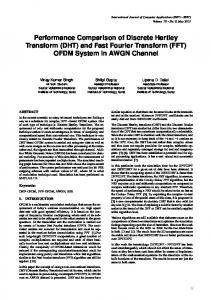
Figure 3. The frequency spectrum for Question 2b (exp (-1206;rt) enters the spectrum from the right and is 53 Hz away from the right boundary; note the amplitude differences).
(a) s () = sin (I00;rt) +sin (70;rt) ? t4
SM:) FmrowMv r4m"ns of 8#t)
(b) s(t)
=sin(86;rt)+exp(-j206irt)?
(c) s (t)
=
I.
exp (jIO47rt) + sin (1 041rt)?
exp(j21r520)
Answer:
~sin(27c52t)
B
Figures 2-4 show the frequency spectra one should observe with the given parameters.
S
0.4-
3. At which frequencies do you observe the signal (and why) if At =40ms and T =0.21 s for
ni
(a) s (t) = sin (IO0rt)+ exp (j70grt) ?
0.41
S9iFn
wres -pons
0.2
f O.4*,
20
30
40
50
Figure 4. The frequency spectrum for Question 2c (exp(jl04;rt) enters the spectrum from the left and is 2Hz away from the left boundary).
bfsQ
0.4 0,351
(b) s ()
sin(21r3t)
=
exp (j32;rt) +sin (867rt) ?
(c) s (t) = exp (jl 2Oirt)+exp,(j206;t)? 0.r
The answers to these three questions are left to the reader. Use any of the two MATLAB scripts listed in Tables 2 and 3, and observe the frequency spectra yourself.
0.15101
00M 1o
-40
-30
-20
40
0
10
20
30
40
50
Figure 2. The frequency spectrum for Question 2a (±50 Hz cannot be observed since these frequencies exactly appear at
242
7. Conclusions The Fourier transform is an important procedure in engineering. The DFT and FFT are discrete tools to analyze time-domain signals. One needs to know the problems caused because of the discretization, and to specify' the parameters accordingly to avoid IEEE Antennas and Propagation Magazine, Vol. 49, No. 3, Juno 2007
nonphysical and nornmathematical results. Moreover, extra attention should be paid when using built-in commands in different computer languages (e.g., MATLAB). As pointed out above, one needs to multiply the results of the FFT taken using MATLAB's ift (s, N) command with At in order to obtain correct amplitude values. Another MATLAB example is the convolution command. The command conv (A, B) convolves vectors A and B. The result is a vector with the size of length(A) +length(B) - 1. The reader may naturally assume that this information is adequate. Again, when you attempt to convolve two discrete time signals, you realize that you are in trouble. The convolution of two discrete time signals, each with N samples and At sampling intervals, one extending from tj to t2 and the other from t3 to t 4 , is another time signal
that extends from t1 + t3
to t2 + t 4 having 2N 1 samples with the same At sampling interval. Again, one needs to multiply the results by At in order to obtain correct amplitude values.
A nice Lab View-based virtual FFT tool has been developed for novel engineering labs to exercise all Fourier-transform-related problems. It targets undergraduate- and graduate-level engineering students (visit http://www3.dogus.edu.tr/lsevgi for this virtual tool and many others; they can freely be downloaded).
IEEE Antennas and Propagation Magazine, Vol. 49, No. 3, June 200724
8. References 1. Baron Jean Baptiste Fourier http:/Ibartleby.com/65/fo/Fouriers.htmnl).
(see,
e.g.,
2. HP, "The Fundamentals of Signal Analysis," Hewlett Packard Application note 243, 1994. 3. L. Sevgi, F. Akleman, and L. B. Felsen, "Ground Wave Propagation Modeling: Problem-Matched Analytical Formulations and Direct Numerical Techniques," IEEE Antennas and Propagation Magazine, 44, 1, February 2002, pp. 55-75. 4. L. Sevgi, Complex Electromagnetic Problems and Numerical Simulation Approaches, New York, IEEE Press/John Wiley and Sons, June 2003. 5. M. Levy, Parabolic Equation Methods for Electromagnetic Wave Propagation,London, IEE, 2000. 6. F. J. Hamrs, "On the Use of Windows for Harmonic Analysis with the Discrete Fourier Transform," Proc. IEEE, 66, 1, January 1978, pp. 51-83. 7. L. Sevgi and Q. Ului~ik, "A Labview-Based Virtual Instrument for Engineering Education: A Numerical Fourier Transform Tool," ELEKTRIK, Turkish J1 of Electrical Engineering and Computer Sciences, 14, 1, 2006, pp. 129-152. l
243