Numerical Investigation of Hydrodynamic Stability of

AIAA SciTech Forum 8–12 January 2018, Kissimmee, Florida 2018 AIAA Aerospace Sciences Meeting

10.2514/6.2018-0586

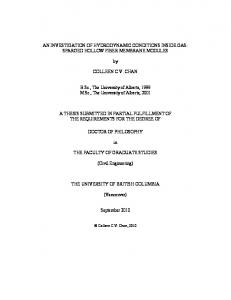
Numerical Investigation of Hydrodynamic Stability of Inward Radial Rayleigh-B´ enard-Poiseuille Flow M. K. Hasan∗ and A. Gross†

Downloaded by Andreas Gross on March 5, 2018 | http://arc.aiaa.org | DOI: 10.2514/6.2018-0586

Mechanical and Aerospace Engineering Department, New Mexico State University, Las Cruces, NM 88003

Since the generation of green and clean renewable energy is a major concern in the modern era, solar energy conversion technologies such as the solar chimney power plant are gaining more attention. In order to accurately predict the performance of these power plants, hydrodynamic instabilities that can lead to large-scale coherent structures which affect the mean flow, have to be identified and their onset has to be predicted accurately. The thermal stratification of the collector flow (resulting from the temperature difference between the heated bottom surface and the cooled top surface) together with the opposing gravity can lead to buoyancy-driven instability. As the flow accelerates inside the collector, the Reynolds number can get large enough for viscous (Tollmien-Schlichting) instability to occur. A new highly accurate compact finite difference Navier-Stokes code in cylindrical coordinates has been developed for the spatial stability analysis of such radial flows. The new code was validated for a square channel flow. Stability results for different stable and unstable Reynolds/Rayleigh number combinations were in good agreement with temporal stability simulations as well as linear stability theory. To investigate the radial flow effect, spatial stability simulations were then carried out for a computational domain with constant streamwise extent and different outflow radii. The Reynolds and Rayleigh number were chosen such that buoyancy-driven instability occured. For cases with significant radial flow effect, the spatial growth rates of the azimuthal modes were found to vary considerably in the streamwise direction.

I.

Introduction

Energy is one of the most essential commodities for human beings to survive and strive. The technological advancement as well as the economic growth of a country rely heavily on the efficient production and use of energy. However, harnessing non-renewable energy resources, for example, fossil fuels, coal, petroleum and natural gas etc. adds to the pollution of the environment and may be an important contributor to global warming which is one of the biggest concerns in the contemporary world. This provides the motivation to tap renewable energy resources that do not pollute the atmosphere and that are replenished naturally over time. The solar chimney power plant (SCPP) is a propitious and attractive technology for converting irradiated solar energy, one of the dominant renewable energy resources, into electrical power. Moreover, it is well suited for desert areas, sun-rich wastelands, and other arid regions. The lack of need for conventional fuel or water, the low-tech construction and the low technical complexity compared to other solar power conversion technologies, make SCPPs interesting and attractive.1 The SCPP represents an appealing alternative for producing green renewable energy. It is a system that converts solar thermal energy using a combination of three components (collector, chimney, and turbine). A small fraction of the solar irradiation is reflected or absorbed by the collector cover. Most of the irradiation passes through the cover and is absorbed by the ground. The air, which is the working fluid in the system, is heated by the ground inside the collector (greenhouse effect). The hot air is less dense than the surrounding ambient air. The density difference results in a buoyancy force that drives the hot air through a central chimney, thus transforming part of the thermal energy into kinetic energy. Turbines installed at the chimney entrance convert a large part of the kinetic energy of the hot air into mechanical energy which is then turned ∗ Graduate † Assistant

Research Assistant. Member AIAA. Professor. Senior Member AIAA.

1 of 20 American Institute of Aeronautics and Astronautics Copyright © 2018 by the authors. Published by the American Institute of Aeronautics and Astronautics, Inc., with permission.

into electrical power through generators. The power generated by SCPPs scales with the product of the collector area and the chimney height.2 This volumetric scaling is a distinctive advantage compared to other power plants where the power scales with the area. A demonstration SCCP that was designed and built by Schlaich, Bergermann and Partner in Manzanares, Spain (1982-1989) generated approximately 50kW of electrical power.2–5 According to Schlaich,2 the generated electrical power can be estimated according to


2 Ht πRc2 I , P = ηc ηt g 3 cp T∞

(1)

where ηc and ηt are the collector and turbine efficiency, g is the gravitational acceleration, I is the solar irradiation, and T∞ is the ambient temperature. The generated power scales with the collector area, πRc2 and the chimney height, Ht . Channel flows with temperature gradient and opposing gravity in the vertical direction are referred to as Rayleigh-B´enard-Poiseuille (RBP) flows. Research on the stability of RBP flows has been carried out over many years. Gage and Reid6 analyzed the linear temporal stability of plane RBP flows and provided neutral curves for the onset of buoyancy-driven instability (critical Rayleigh number, Rac =1,708) and viscous (Tollmien-Schlichting) instability (critical Reynolds number, Rec =5,400). When the Reynolds number is below Rec =5,400 and the Rayleigh number is larger than Rac =1,708, buoyancy-driven instability occurs and three-dimensional (3-D) waves with a wave angle of 90deg are amplified; For Re > Rec and Ra < Rac , viscous instability occurs and two-dimensional (2-D) Tollmien-Schlichting waves with a wave angle of 0deg are amplified. When the distubances are allowed to grow to nonlinear amplitudes, streamwise (longitudinal) flow structures are expected to form for the former and spanwise (transverse) structures are expected to appear for the latter. Various numerical7 and experimental8 investigations support the findings by Gage and Reid.6 Mori and Uchida9 investigated the forced convective heat transfer between horizontal flat plates and observed counter-rotating longitudinal vortices when the temperature difference between the plates was increased above a critical value. Fukui and Nakajima10 considered free and forced laminar convection flows between horizontal and inclined parallel plates and focused on the effect of longitudinal rolls on the transport processes. A combined experimental and computational study for a range of channel aspect ratios, thermal boundary conditions (inlet as well as walls), and Reynolds and Rayleigh numbers was carried out by Mergui et al.11 The number of longitudinal vortices for a given aspect ratio was found to be independent of the Rayleigh and Reynolds number. Fujimura and Kelly12 investigated the nonlinear interaction of longitudinal and transverse flow structures. Below the critical Reynolds number (Re < Rec ), the flow was found to become unstable and longitudinal vortex rolls developed, provided that the Rayleigh number was high enough and the spanwise extent of the channel was infinite. The effect of the spanwise or transversal extent of the channel on the instability of plane RBP flows has also received considerable attention in the literature. Luijkx et al.13 suggested that when the Reynolds number is below its critical value (no viscous instability), transverse rolls are favored over longitudinal rolls for aspect ratios (width to height) of less than five. Nicolas et al.14 also found that transverse rolls are preferred for low aspect ratio plane RBP flows. Furthermore it was shown that reducing the aspect ratio has a stabilizing effect and raises the critical Rayleigh number, Rac , for the buoyancy-driven instability. An experimental analysis of the hydrodynamic instability of RBP flows with large aspect ratio was conducted by Grandjean and Monkewitz.15 They reported that the appearance of transverse rolls is triggered by the transition from a convective to an absolute instability. The flow in the collector of the SCPP constitutes an inward radial RBP flow. Unlike for the square channel flow, for the inward radial channel flow the velocity strongly increases in the streamwise direction (close to 1/r-relationship because of radial continuity equation) and the flow is non-parallel in planes parallel to the walls. Assuming that the radial velocity in the chimney behaves according to v ' r1 v1 /r where r1 and v1 are the radius and velocity at the collector inlet, the radial acceleration behaves according to a ' (r1 v1 )2 /r3 . Since acceleration is typically stabilizing,16 the hydrodynamic stability of the inward radial RBP flow is expected to differ significantly from the hydrodynamic stability of the plane RBP flow especially for small r. The understanding of the hydrodynamic instabilities of radial RBP flows (both primary and secondary) is of vital importance for the design of SCPP plants as it provides the critical parameters (such as Reynolds number, Rayleigh number, Prandtl number) that determine if and where coherent flow structures will form. Coherent flow structures modify the overall heat transfer and pressure drop in the collector and thus will have a profound effect on the SCPP performance. Because of its great promise as an alternative energy source, the SCPP technology has been investigated by numerous researchers over several decades. Bernardes et al.17 were the first to present a numerical analysis 2 of 20 American Institute of Aeronautics and Astronautics


of the natural laminar convection in a SCPP. They investigated the effect of different geometric configurations such as a straight, curved and slanted junction as well as a conic chimney and curved junction/diffuser on the thermo-hydrodynamic behavior. It was observed that a conic chimney geometry resulted in a greater mass flow rate and higher temperatures at the outlet. Pastohr et al.18 used the Manzanares prototype as a reference for analytical calculations and Reynolds-averaged Navier-Stokes (RANS) calculations. They found that the pressure drop across the turbines and the mass flow rate through the chimney had a profound impact on the SCPP efficiency. Ming et al.19–21 performed RANS calculations and investigated the effect of various parameters on the differential pressure between chimney and atmosphere, the efficiency of the SCPP, and the effect of crosswind on the SCPP performance. A numerical analysis of the heat transfer, the generated power and energy loss, and the turbine pressure drop has been carried out by Xu et al.22 Koonsrisuk and Chitsomboon23 performed a numerical investigation of the relationship between the generated power and the collector and chimney geometry and suggested that the combination of a sloping collector roof and a divergent chimney can greatly enhance the power output. Fasel et al.24 employed RANS calculations for investigating the validity of the cubic scaling law for the generated power. Nia and Ghazikhani25 employed passive flow control for improving the heat transfer in the collector. An observed increase of the generated power was attributed to a stronger wall-normal mixing. Longitudinal structures arising from buoyancydriven instability are expected to have a similar effect on the heat transfer. Shirvan et al.26 performed a numerical simulation and sensitivity analysis to examine the effect of various parameters such as the collector entrance gap, chimney diameter, chimney height, and inclination of the collector roof on the maximum power production. The generated power was found to be proportional to the chimney diameter and chimney height and inversely proportional to the collector entrance gap. Hu et al.27 investigated the effect of the chimney geometry on the generated power output. Van Santen et al.28, 29 carried out simulations and experiments of a forced radial outward flow with buoyancy-driven convection. Axisymmetric 3-D transverse rolls appeared for very low Reynolds numbers when the Rayleigh number was above the critical value. This is an interesting finding since in accordance with Gage and Reid6 longitudinal vortices should be favored when the Reynolds number is below its critical value. The Van Santen et al.28, 29 results thus indicate that the stability of radial RBP flows may be different from the stability of plane RBP flows. Fasel et al.30 investigated the RBP flow in the collector of a 1:33 scale Manzanares SCPP and discovered transverse rolls near the collector inlet and streamwise longitudinal vortices near the collector outlet. Similar observations were also made by Meng et al.31 Recently, Bernardes32 investigated the stability of the converging flow between two approximately parallel fixed disks (a configuration that resembles the collector of a solar chimney power plant). Natural convection and vortex rolls were observed towards the collector outlet when the Richardson number exceeded a critical value. Temporal stability simulations for plane RBP flows by Hasan and Gross33 laid the foundation for the stability simulations of radial RBP flows that constitute the main contribution of this paper. Towards this end, a newly developed highly accurate compact finite difference computational fluid dynamics (CFD) code in Cartesian coordinates was modified to allow for simulations of radial flows. Additional temporal stability simulations of plane RBP flows (square channel) were performed to obtain validation data for the new code and reference data for a comparison with the spatial radial flow simulations. The radial flow effect (radial acceleration) for the spatial simulations was varied by keeping the streamwise domain extent constant and varying the outflow radius. Based on a detailed analysis of the azimuthal mode amplitudes and growth rates, a qualitative understanding of the radial flow effect on the stability characteristics is gained.

II.

Methodology

Details on the Navier-Stokes code in Cartesian coordinates for square channel RBP simulations can be found in an earlier paper.33 The discussion here focuses on the extension of the code to cylindrical coordinates. All simulations were performed on a local work station. A.

Governing Equations

The code solves the compressible Navier-Stokes equations or more specifically the conservation equations for mass, momentum, and total energy. According to Sandberg,34 the governing equations in cylindrical coordinates are, ∂U ∂A ∂B 1 ∂C 1 + + + + D = H, (2) ∂t ∂z ∂r r ∂θ r 3 of 20 American Institute of Aeronautics and Astronautics

with state vector,  ρ  ρu       ρv  ,   ρw  U=

(3)

ρe and flux vectors,  ρu   ρu2 + p − τzz     ,  ρuv − τrz     ρuw − τθz u(ρe + p) − uτzz − vτrz − wτθz + qz   ρv   ρvu − τrz     ,  ρv 2 + p − τrr     ρvw − τθr v(ρe + p) − uτrz − vτrr − wτθr + qr   ρw   ρwu − τθz      . ρwv − τθr     ρw2 + p − τθθ 


A=

B=

C=

(4)

(5)

(6)

w(ρe + p) − uτθz − vτθr − wτθθ + qθ Here, u, v, and w are the velocities in the z (wall-normal), r (streamwise), and θ (azimuthal) direction, ρ is the density, and p is the static pressure. The total energy is e = + 1/2(u2 + v 2 + w2 ), where = cv T is the internal energy, cv is the specific heat at constant volume, and T is the temperature. The source term vectors are   ρv   ρuv − τrz     D=  (7) , ρv 2 − ρw2 − τrr + τθθ     2ρvw − 2τθr v(ρe + p) − uτrz − vτrr − wτθr + qr and  H=

0



 g(ρ  ref − ρ)      . 0     0 ug(ρref − ρ)

(8)

Vector H contains a buoyancy term (Boussinesq approximation), g(ρref −ρ), with gravitational acceleration, g = 9.81m/s2 . The shear stress tensor components are, 2 ∂u ∂v 1 ∂w τzz = µ 2 − − +v , (9) 3 ∂z ∂r r ∂θ ∂u ∂v 1 ∂w 2 τrr = µ − +2 − +v , (10) 3 ∂z ∂r r ∂θ 2 ∂u ∂v 1 ∂w τθθ = µ − − +2 +v , (11) 3 ∂z ∂r r ∂θ

4 of 20 American Institute of Aeronautics and Astronautics

and

τθr

∂u ∂v τrz = µ + , ∂r ∂z ∂w 1 ∂u τθz = µ + , ∂z r ∂θ 1 ∂v ∂w =µ −w + , r ∂θ ∂r

(12) (13) (14)

with dynamic viscosity, µ. The heat flux vector components are, qz = −k

∂T , ∂z

(15)

∂T , ∂r 1 ∂T qθ = −k , r ∂θ with heat conduction coefficient, k. The set of equations is closed by the ideal gas equation,


qr = −k

p = ρRT,

(16) (17)

(18)

with gas constant, R, and Sutherland’s law for the viscosity. B.

Non-Dimensionalization

The governing equations were made dimensionless with a reference velocity, vref , a reference length scale, Lref , a reference temperature, Tref , and a reference density, ρref . Pressure was made dimensionless with 2 ρref vref . The Reynolds number based on bulk velocity and hydraulic diameter is Re =

ub 2h , ν

(19)

where h is the channel height. For the present simulations the bulk velocity was taken as reference velocity, vref = ub , and the channel half-height was taken as reference length, Lref = h/2. The resulting reference Reynolds number is ub h2 vref Lref 1 Reref = = = Re . (20) ν ν 4 The Rayleigh number is defined as γh3 g∆T Ra = , (21) να where γ = 1/Tav with Tav = (Thot + Tcold )/2 is the thermal expansion coefficient for a perfect gas, ∆T = Thot − Tcold , is the temperature difference between the bottom and top wall, and α is the thermal diffusivity. The Prandtl number is defined as ν (22) Pr = . α For the chosen reference quantities, the Rayleigh number can be rewritten as ∆T 2 Tav

Ra = Re

3

h Lref

Pr

L

g v2ref ref

,

(23)

2 where gLref /vref is the dimensionless gravitational acceleration. The specific heats are cp = γ/[(γ − 1)M 2 ] and cv = 1/[γ(γ − 1)M 2 ] and the gas constant is R = cp − cv = 1/(γM 2 ), where M is the Mach number. The heat conduction coefficient is k = µ/[P r(γ − 1)M 2 Re], where P r is the Prandtl number.


C.

Discretization

The first and second derivatives in the radial direction were discretized with fourth-order-accurate compact finite differences, 0 0 fi−1 + 4fi0 + fi+1

=

00 00 fi−1 + 10fi00 + fi+1

=

3fi+1 − 3fi−1 ∆r 12fi+1 − 24fi + 12fi−1 . ∆r2

(24) (25)

Fourth-order-accurate compact finite differences for non-uniform grids by Shukla et al.,35 (d)

(d)

ai−1 fi−1 + fi

(d)

+ ai+1 fi+1

= bi−1 fi−1 + bi fi + bi+1 fi+1 ,

(26)


were employed in the wall-normal direction. Here d (either one or two) symbolizes the order of the derivative. The coefficients are provided in Tab. 1 where hi = zi −zi−1 is the wall-normal grid line spacing. The resulting d=1

d=2

ai−1

hi+1 2 { hi+1 +hi }

ai+1

{ hi+1hi+hi }2

h2 +h h −h2i+1 i+1 } { hih+h }{ h2i+3hii hi+1 +h2i+1 i+1 i+1 i 2 2 h +hi hi+1 −hi hi } { hi +h }{ h2i+1 2 i+1 i +3hi hi+1 +hi+1

bi−1 bi bi+1

2h2i+1 {2hi +hi+1 } hi {hi+1 +hi }3 2{hi+1 −hi } hi hi+1 2h2i {hi +2hi+1 } hi+1 {hi+1 +hi }3

−

i+1 }{ h2 +3hi h12 } { hih+h 2 i+1 i+1 +h i

i+1

−12 h2i +3hi hi+1 +h2i+1 hi }{ h2 +3hi h12 { hi +h } 2 i+1 i+1 +h i

i+1

Table 1. Coefficients for fourth-order-accurate compact finite difference stencils for non-uniform grids.35

tridiagonal systems of equations in the radial and wall-normal directions were solved with the Thomas algorithm. Derivatives in the periodic azimuthal (θ-coordinate) direction were calculated in Fourier space.33 The forward and backward Fourier transforms were computed with fast Fourier transforms (FFTs).36, 37 When the flux derivatives are brought to the right-hand-side, the governing equations can be written as, ∂U ∂A ∂B 1 ∂C 1 =R= H− − − − D . (27) ∂t ∂z ∂r r ∂θ r A fourth-order-accurate explicit low-storage Runge-Kutta method38 was employed for time integration, Q1 Q2 Q1 Q2 Q1 Qn+1

∆t R(Qn ) 2 ∆t R(Q1 ) = Qn + 2 ⇐ Q1 + 2Q2 =

Qn +

Qn + ∆tR(Q2 ) 1 ⇐ (−Qn + Q1 + Q2 ) 2 ∆t = Q1 + R(Q2 ) . 6

(28)

(29)

=

(30) (31)

Here, n and n + 1 are the old and new time step. D.

Boundary Conditions

Flow periodicity was enforced in the azimuthal direction. Isothermal no-slip and no-penetration boundary conditions were employed at both walls. The wall-normal pressure gradient at the wall was computed as33 ∂p = g(1 − ρ) . ∂z 6 of 20 American Institute of Aeronautics and Astronautics

(32)


The one-sided derivative was discretized with a fourth-order-accurate compact finite difference stencil. Nonreflecting boundary conditions based on Riemann invariants39 were employed at the inflow boundary. The outgoing and incoming characteristic at the inflow boundary are, R + = vi +

2ci , γ−1

(33)

R − = va −

2ca . γ−1

(34)

The internal velocity, vi , and speed of sound, ci , at the boundary were extrapolated from inside the computational domain assuming zero fourth derivatives, ∂ 4 /∂r4 = 0 (the derivatives were discretized with fourth-order-accurate one-sided finite difference stencils). The subscript “a” denotes the known ambient state. The entropy at the inflow boundary was taken as sb = c2a /(γργ−1 ) and the velocity and speed of a sound were computed from 1 (35) vb = (R+ + R− ) , 2 and γ−1 + cb = (R − R− ) . (36) 4 The remaining flow quantities were computed as c2b γsb ρb c2b , γ

ρb

=

pb

=

1 γ−1

,

(37) (38)

and Tb = (M cb )2 . A characteristics-based boundary condition by Gross and Fasel40 was employed at the outflow boundary. A shooting method was employed to solve the equations describing one-dimensional laminar RBP flow, ∂p ∂2u =µ 2, ∂x ∂y

(39)

∂p = (1 − ρ)g , ∂y

(40)

2 ∂2T ∂u k 2 +µ = 0. ∂y ∂y

(41)

The equations were derived from the 3-D incompressible Navier-Stokes equations in Cartesian coordinates assuming parallel flow (∂/∂x = 0, where x is the streamwise coordinate), a zero wall-normal (y-direction) velocity (v = 0), and steady flow (∂/∂t = 0). The computed profiles provided the ambient values for the inflow and outflow boundary conditions. E.

Computational Domain

A coordinate transformation that clusters grid points near the walls was employed in the wall-normal direction (grid line index: j, total number of points: J), tan−1 (jc − f1 ) h zj = +1 × , (42) f2 2 where h = 2 is the channel height, f1 = Jc/2 and f2 = tan−1 (f1 ), and c=0.1 is a user specified constant. Equidistant grid point distributions were employed in the streamwise and azimuthal directions. The streamwise extent (length) of the computational domain was L=12 for the square channel flow simulations and L=10 for the radial flow simulations. The spanwise grid extent at the inflow boundary was Z=12 (Fig. 1). 7 of 20 American Institute of Aeronautics and Astronautics

a)

b)


Figure 1. (a) Computational domain boundaries and (b) details of mesh for square channel flow simulations.

b)

a)

Figure 2. (a) Computational domain boundaries and (b) details of mesh for inward radial channel flow simulations.

Different outflow and inflow radii were chosen for the radial channel flow simulations. In Fig. 2a a computational domain with outflow boundary at r1 = 3 and inflow boundary at r2 = 13 is shown. The azimuthal extent of the inflow boundary (arclength) was held constant at 12 for all radial channel flow simulations. The azimuthal grid opening angle was adjusted accordingly, ∆θ = s/r2 . The number of grid points in the streamwise and wall-normal direction was 32 and 49, respectively. For the 3-D simulations, 32 collocation points were used in the spanwise/azimuthal direction. F.

Linear Stability

In linear stability theory a wave ansatz, v 0 = V (y)ei(αx+βz−ωt) ,

(43)

is made for the disturbances with streamwise wavenumber, α=αr +iαi , spanwise wavenumber, β=βr +iβi and frequency, ω=ωr +iωi . The real part of the streamwise and spanwise wavenumbers is related to the wavelengths via αr = 2π/λx and βr = 2π/λz ; The real part of the frequency is related to the period, ωr = 2π/T . Since λx = L/l and λz = Z/k, the modes can also be referenced by their streamwise, l, and spanwise or azimuthal mode number, k. For the present simulations the disturbances grow either in time (temporal simulations) or space (spatial simulations). Temporal growth occurs for ωi > 0 and αi = βi = 0. Spatial growth occurs for αi < 0 and βi = ωi = 0. Different criteria can be chosen for plotting the disturbance amplitudes. For the results shown in this paper, it was decided to show the wall-normal velocity at the mid-channel height. This quantity is zero in the mean for the temporal simulations (parallel flow). For the spatial simulations, a very small non-zero value is obtained because the differential heating makes the flow slightly asymmetric in the wall-normal direction. Because of the streamwise and spanwise periodicity of the temporal simulations, the disturbances can easily be Fourier-transformed in both directions, v 0 (x, y, z, t)

= vˆ(y)ei[αr x+βr z−(ωr +iωi )t] = vˆ(y)ei(αr x+βr z−ωr t) eωi t = ei(αr x+βr z−ωr t) A[v 0 (y, t)] . 8 of 20

American Institute of Aeronautics and Astronautics

(44)

The temporal growh rates can then be computed via, ∂lnA(v 0 ) . ∂t Similarly, for the spatial simulations the growth rates are obtained from ωi =

αi = −

∂lnA(v 0 ) , ∂s

(45)

(46)

where s is the arclength in the streamwise direction, s = r2 − r . G.

(47)

Defining Parameters for Different Cases


The bottom and top wall temperature were held constant at 350K and 300K, respectively. The latter was also chosen as reference (ambient) temperature. The reference Mach number was set to 0.3 for the square channel flow simulations and 0.05 for the radial channel flow simulations. In accordance with Gage and Reid,6 the Prandtl number was set to 1.

Figure 3. Investigated cases (symbols and dashed lines) plotted in stability diagram by Gage and Reid.6

Various stable and unstable cases were set up according to the neutral curves provided by Gage and Reid6 (Fig. 3). For the radial RBP flow cases, the velocity and hence the Reynolds number are changing in the streamwise direction and the cases thus appear as horizontal lines in Fig. 3. According to Gage and Reid,6 when the Reynolds number is less than its critical value (Re < Rec =5, √ 400, black line in Fig. 3) and the Rayleigh number is greater than its critical value (Ra > Rac =1, 708, Rac = 41.3, brown line in Fig. 3), buoyancy-driven instability occurs. According to the Gage and Reid6 stability diagram, 3-D modes become unstable first when the Rayleigh number is increased above its critical value. However, when 3-D disturbances are artificially suppressed (such as in 2-D simulations), the λ=0deg neutral curve (black line) determines the onset of buoancy driven instability. A total of fifteen cases (Tab. 2) were investigated. The cases were chosen such that the flow is either (1) stable, (2) unstable w.r.t. 3-D waves, or (3) unstable w.r.t. 2-D waves (3-D waves are suppressed). Eleven simulations were performed with the new spatial Navier-Stokes code in radial coordinates. In addition, temporal flow simulations were carried out with a code in Cartesian coordinates that employs Fourier transforms in the streamwise direction.33 To allow for a direct comparison with the temporal simulations, for some of the spatial simulations the outflow radius was set to 107 to obtain a nominally 2-D flow (Tab. 2). For all cases, a steady basic flow was computed first. Very small (linear) disturbances were then introduced inside the domain (temporal simulations) or at the inflow boundary (spatial simulations). 9 of 20 American Institute of Aeronautics and Astronautics


Case 1 Case 2 Case 3 Case 4 Case 5 Case 6 Case 7 Case 8 Case 9 Case 10 Case 11 Case 12 Case 13 Case 14 Case 15

Dimensions 3-D 3-D 3-D 3-D 2-D 2-D 2-D 2-D 3-D 3-D 3-D 3-D 3-D 3-D 3-D

Re 30 30 30 30 100 100 100 100 30 30 30 30 30 30 30

√

Ra 100 100 30 30 300 300 100 100 100 100 100 100 100 30 30

Code Temporal Spatial Temporal Spatial Temporal Spatial Temporal Spatial Spatial Spatial Spatial Spatial Spatial Spatial Spatial

Geometry Square Square Square Square Square Square Square Square Radial Radial Radial Radial Radial Radial Radial

Inflow radius (r2 ) 107 +10 7 10 +10 7 10 +10 7 10 +10 110 60 35 15 13 60 110

Outflow radius (r1 ) 107 107 107 107 100 50 25 5 3 50 100

Table 2. Parameters for 2-D and 3-D simulations. For spatial simulations, Re is inflow Reynolds number.

III. A.

Results

Validation Cases

Four temporal (cases 1, 3, 5, and 7) and four spatial (cases 2, 4, 6, and 8) square RBP flow simulations were performed and the stability behavior was compared. For the √ spatial√simulations the outflow radius was set to 107 to simulate a square channel flow. For cases 1 & 2, Ra > Rac = 41.3 and 3-D disturbances (λ=90deg) are expected to grow. Cases 3 & 4 are expected to be stable. For cases 5 & 6, the Rayleigh number 6 is above the λ=0deg neutral curve √ in the Gage and Reid stability diagram (Fig. 3) and 2-D disturbances are expected to grow. Although Ra > 41.3 for cases 7 & 8, these cases are expected to be stable since 3-D disturbances are artificially suppressed in the 2-D simulations.

a)

b)

Figure 4. a) Time evolution of spanwise Fourier modes of wall-normal velocity at mid-channel height and b) growth rates for case 1 (unstable).

The spanwise disturbance mode amplitudes and growth rates for case 1 are shown in Fig. 4. As expected based on the Gage and Reid6 stability diagram, the flow is unstable and spanwise modes k=1-7 are growing exponentially (linear growth). The spanwise mode k=4 has a constant growth rate of ωi ≈0.33 (Fig. 4b) and



saturates around t ≈ 110. Spanwise modes k=5 and k=3 also exhibit strong linear growth. For t > 50 the growth rates of modes 1, 2, 6, and 7 suddenly increase, possibly as a result of resonances or non-linear effects. From t≈53.3 to t≈96.58 mode k=2 has the highest growth rate (Fig. 4b). However, mode k=4, which has a spanwise wavelength of λz = 12/4 = 3, remains dominant (highest amplitude). In Fig. 5a the growth rates of modes 2, 3, 4 & 5 are plotted over the time interval 22 < t < 42. Mode 4 with spanwise wavenumber β=2.1 has the highest growth rate (Fig. 5b). A visualization of the flow field at t=150 reveals 8 counter-rotating longitudinal vortices (Fig. 6). Shown are iso-surfaces of the Q-criterion41 flooded by the streamwise vorticity. In Fig. 7 spanwise Fourier modes of the wall-normal velocity at the mid-channel height are plotted for case

a)

b)

Figure 5. Growth rates of spanwise modes versus a) time and b) spanwise wavenumber (at t=31.9) for case 1 (unstable).

Figure 6. Iso-surfaces of Q=0.2 flooded by streamwise vorticity (ωx ) for t=150 (case 1).

3. In agreement with Gage and Reid,6 all Fourier modes decay over time. The first spatial stability simulations for case 2 indicated that the flow response to the disturbance input at the inflow boundary depended on the disturbance mode shape (receptivity). For certain disturbance mode shapes, linear growth was either not observed at all or occured close to the outflow boundary. It was therefore decided to first extract the saturated disturbance modes from case 1 (unstable temporal simulation), to then rescale them to a maximum wall-normal disturbance velocity of 5.1×10−11 , and finally, to superimpose them on the ambient conditions at the inflow boundary for the spatial simulations. For all spatial cases, the simulations were terminated when the flow field did no longer change in time. In Fig. 8 the spanwise Fourier modes of the wall-normal disturbance velocity at the mid-channel height are plotted versus the arclength for case 2. Modes 3-7 exhibit linear growth (Fig. 8a). Modes 2 and 1 grow for s > 2 possibly as a result of resonances or nonlinear effects. In agreement with the temporal simulation for case 1, mode 4 has the largest growth rate (most negative αi for 6.5 < s < 8.5) followed by modes 3 and 5 (Fig. 9). The temporal and spatial growth rates are related via the Gaster transform.42 Since the wave speeds are unknown (the longitudinal structures are steady) no attempt was made at employing the Gaster 11 of 20 American Institute of Aeronautics and Astronautics


Figure 7. Time evolution of spanwise Fourier modes of wall-normal velocity at mid-channel height for case 3 (stable).

a)

b)

Figure 8. a) Spatial evolution of spanwise Fourier modes of wall-normal velocity at mid-channel height and b) growth rates for case 2 (unstable).

Figure 9. Growth rates of spanwise modes versus spanwise wavenumber (s=7.42) for case 2.



transform for comparing the temporal and spatial stability results. For case 4 (Fig. 10), in agreement with case 3, all disturbances are damped.

Figure 10. Spatial evolution of spanwise Fourier modes of wall-normal velocity at mid-channel height for case 4 (stable).

a)

b)

Figure 11. a) Streamwise and b) temporal Fourier modes of wall-normal velocity at mid-channel height for cases 5 & 7 (temporal simulations) and 6 & 8 (spatial simulations). 6 Results for the 2-D simulations (cases 5-8) are shown in Fig. 11. √ In agreement with Gage and Reid, linear growth (unstable) is observed for case 5 (since the chosen Re- Ra combination is above the λ=0deg neutral curve in Fig. 3) and linear decay is observed for case 7 (stable in Fig. 11a). The saturated disturbance mode was extracted from the case 5 temporal simulation. The mode was rescaled to a maximum wall-normal velocity of 3×10−4 and introduced at the inflow boundary of the spatial simulations. The inflow disturbance frequency was set to 0.63 which is the frequency of the unstable mode in the temporal simulation. For cases 6 & 8 the disturbance amplitudes undergo some adjustment at the inflow and outflow boundaries (Fig. 11b). This behavior is most likely a consequence of the chosen boundary conditions. Other than that, the results are in qualitative agreement with the temporal simulations and with Gage and Reid.6

B.

Inward Radial Flow Stability Simulations

Based on the good qualitative agreement of the temporal and spatial stability simulations for the square channel, it was decided to employ the Navier-Stokes code in cylindrical coordinates for spatial stability simulations of inward radial flows. The intent of the radial stability simulations was to determine whether the neutral curves by Gage and Reid6 remain valid for the inward radial RBP flow. In accordance with



the radial continuity equation, the radial velocity in the collector exhibits an almost hyperbolic behavior. Because acceleration is typically stabilizing and because non-parallel effects are present (the profiles change in the streamwise direction) the neutral curves by Gage and Reid6 are expected to be only approximately applicable to inward radial RBP flows. The discrepanices are expected to get larger the closer the outflow boundary is located near r=0. Therefore, a series of spatial simulations was carried out where the streamwise extent of the domain, r2 − r1 , was kept fixed at ten while the outflow boundary location, r1 , was successively reduced from 100 to 3 (cases 9-15, Tab. 2). The outflow boundary was placed at r1 =100 for cases 9 & 15, at 50 for cases 10 & 14, at 25 for case 11, at 5 for case 12, and at 3 for case 13.√ For cases √ 9-13 the inflow Reynolds number was Re = 30 and the square root of the Rayleigh number was Ra > Rac = 100. According to Gage and Reid6 these cases are therefore expected to be unstable (Fig. 3). Cases 14 & 15 are √ √ expected to be stable (Re = 30 and Ra = 30 < Rac ).

a)

b)

Figure 12. a) Azimuthal Fourier modes of wall-normal disturbance velocity at mid-channel height and b) growth rates for case 9.

a)

b)

Figure 13. a) Azimuthal Fourier modes of wall-normal disturbance velocity at mid-channel height and b) growth rate for case 10.

Azimuthal Fourier modes of the wall-normal velocity and growth rates for case 9 are plotted in Fig. 12. Mode 5 has the largest amplitude for 2.25 < s < 9. For s > 2 the growth rate of mode 4 surpasses that of mode 5 (Fig. 12b). Overall, the case 9 results are similar to the results for the square channel flow (Fig. 8). For case 10 (decreased outflow radius, r1 =50) mode 4 reaches a higher amplitude at saturation (Fig. 13a). The changes in the growth rates in the streamwise direction for case 10 (Fig. 13b) are larger than for case 9 (Fig. 12b). For example, the growth rates for modes 5-7 are decreasing more quickly in the streamwise direction for case 10. Because the mode 4 growth rate for both cases is approximately the same, this explains


why mode 4 becomes dominant near the outflow for case 10.


a)

b)


a)

b)


The outflow radius was then decreased to r1 =25 (case 11) and 5 (case 12). The reference Reynolds number, square root of the Rayleigh number, and inflow arc-length remained the same as for case 9. For case 11 (Fig. 14a), mode 5 is dominant first (2 < s < 6.5) and mode 4 is dominant for s > 6.5. For case 12 (Fig. 15a), mode 5 is dominant for 1.5 < s < 3.5 and followed by mode 4 (dominant for 3.5 < s < 6.5) and mode 3 (dominant for 6.5 < s < 10). The results appear consistent, since as the outflow radius is decreased, the higher modes become less amplified or even damped while the lower modes become more amplified (Figs. 14b & Fig. 15b). Since the stability simulation for the square channel flow revealed that the spatial disturbance growth rate depends on the spanwise wavenumber (Fig. 9) this behavior was expected. As a consequence, the dominant mode changes in the streamwise direction. Alternatively, one may say that as the outflow boundary radius is increased, the square channel flow results are approached (Fig. 8). Another interesting observation is that the growth rates near the inflow boundary (s = 0) are increasing as the outflow boundary is moved towards r = 0. In fact, for case 12 the range of the Fig. 15b ordinate had to be changed compared to cases 10 and 11 (Figs. 13b & 14b) to accommodate the larger growth rates. This suggests that acceleration is destabilizing the buoyancy-driven instability which is counter-intuitive. For case 13, the outflow boundary is at r1 =3, the inflow boundary is at r2 =13, and the grid opening angle is ∆θ = s/r2 = 12/13 = 53deg. As a result, the flow is strongly accelerated in the streamwise direction. In Fig. 16 the local Reynolds number (based on the maximum radial velocity) is plotted over the



Figure 16. Local Reynolds number based on velocity maximum versus streamwise arclength.

Radius, r 13 12 11 10 9 8 7 6 5 4 3

Distance, s 0 1 2 3 4 5 6 7 8 9 10

Local Re 28.50 24.58 23.23 24.04 26.25 29.13 32.83 37.77 44.22 54.14 73.68

Azimuthal arc-length 12 11.07 10.15 9.23 8.30 7.38 6.46 5.53 4.61 3.69 2.77

Table 3. Various local parameters for case 13.

streamwise arclength. Downstream of the inlet the local Reynolds number initially drops slightly below the reference Reynolds number (30) and then increases hyperbolically in the radial direction. The intial drop must be attributed to the inflow boundary condition. A maximum local Reynolds number of 74 is obtained at the outflow boundary. Also as a result of the convergence of the channel, the azimuthal arc-length and the channel aspect ratio (width to height) decrease in the streamwise direction. Table 3 provides the local radius, Reynolds number and azimuthal arc-length (equivalent to span in square channel flow simulations) for several streamwise locations. The square channel flow simulations (case 2) have shown that disturbances with a spanwise wavelength of λz ≈ 3 are the most amplified. Since for the spatial simulations, λz =

r∆θ , k

(48)

one may expect mode, r∆θ (r2 − s)∆θ = , (49) λz λz to experience the strongest amplification at streamwise location, s. The disturbance amplitudes and growth rates for case 13 are plotted in Fig. 17. Modes 3-7 have about equal amplitudes at the inflow boundary. As expected the dominant mode switches to lower mode numbers in the streamwise direction. Unfortunately, the growth rate curves in Fig. 17 do not exhibit clear minima (maximum spatial growth) and therefore the previously proposed relationship for the most amplified spanwise mode (Eq. 49) cannot be confirmed. k=


a)

b)


Figure 17. a) Azimuthal Fourier modes of wall-normal velocity at mid-channel height and b) spatial growth rates for case 13.

a)

b)

Figure 18. a) Spanwise Fourier modes of wall-normal velocity at mid-channel height and b) growth rates obtained from temporal simulations for Reynolds number and spanwise domain widths of Tab. 3.

a)

b)

Figure 19. Azimuthal Fourier modes of wall-normal velocity at mid-channel height for a) case 14 and b) case 15.


√ Additional temporal square channel flow simulations (not listed in Tab. 2, same Ra as for case 13) were performed where the Reynolds number and spanwise domain widths of the different streamwise locations in Tab. 3 were matched. The most amplified spanwise modes for the different cases are plotted in Fig. 18a and the growth rates are provided in Fig. 18b. For Z=11.07, spanwise mode k=4 with a wavelength of λz = 2.76 is the most amplified; For Z=10.15, 9.23 & 8.30, mode k=3 experiences the strongest amplification (the corresponding wavelengths are 3.38, 3.07 and 2.76); For Z ≤ 7.38 mode 2 with λz = 3.69 is the most amplified and finally for Z=3.69 mode 1 (λz = 3.69) is the most amplified. The temporal simulations do thus provide additional evidence that the spanwise wavenumber of the most amplified mode is adjusting according to the local azimuthal extent of the domain. √ Finally, for√cases 14 and 15 the square-root of the Rayleigh number was lowered below its critical value ( Ra=30< Rac =41.3). Figure 19 illustrates that both cases are stable.


Conclusions The radial Rayleigh-B´enard-Poiseuille (RBP) flow in the collector of Solar Chimney Power Plants is potentially susceptive to buoyancy-driven and viscous (Tollmien-Schlichting) instabilities. As a result of mass conservation, the flow is strongly accelerated in the streamwise direction. Gage and Reid6 were the first to provide neutral curves for the buoyancy-driven and viscous instabilities of square RBP flows. How the neutral curves are affected by the radial acceleration remains an open question. Since acceleration is typically stabilizing and also introduces weak non-parallel effects, differences with respect to the squarechannel flow results have to be expected. Spatial stability simulations are proposed as a tool for investigating the stability of radial RBP flows. Towards that end a fourth-order-accurate compressible Navier-Stokes code in cylindrical coordinates has been developed. Spatial simulations for a square channel flow were in good qualitiative agreement with temporal simulations that were carried out with a double-Fourier code (Fourier transforms in the streamwise and spanwise directions).33 The results also agreed with the stability behavior (stable or unstable) predicted by Gage and Reid.6 Spatial stability simulations were then performed for various stable and unstable (w.r.t. the buoyancydriven instability) radial RBP flows. The Reynolds number was kept low enough to avoid the onset of viscous instability. The streamwise and azimuthal (at the inflow boundary) domain extent were held constant and the radial location of the outflow boundary was varied between r1 =100 and 3. For large r1 the squarechannel flow solution is approached. The most unstable azimuthal mode was found to have a wavelength of approximately 3. Since the channel height was normalized to 2, this corresponds to 1.5/2=0.75 vortices per channel height at mode saturation. As the outflow radius was successively reduced, the difference in azimuthal arc-length between the inflow and outflow boundary increased. Because of continuity, this led to an increase of the outflow velocity. However, even when the outflow boundary was placed at r1 =3 (the most “extreme” case), the wavelength of the most amplified azimuthal mode was found to remain close to 3. Although the wavelength of the most amplified mode remained approximately constant in the streamwise direction, the corresponding azimuthal mode number was found to be decreasing (because the azimuthal arc-length of the domain decreases in the streamwise direction). Similar findings were made by Meng et al.31 In the future, the viscous instability of the radial RBP flow will be investigated as well. The viscous instability depends on the local Reynolds number which increases in the streamwise direction. Cases may be perceived where the critical Reynolds number is exceeded somewhere inside the collector. Also of interest are cases with both bouyancy and viscous driven instability where the mode amplitudes are allowed to grow to large enough amplitudes to allow for nonlinear interactions. Finally, a linearization of the spatial code appears desirable to avoid inaccuracies when the disturbance amplitudes are near machine roundoff as well as non-linear mode interactions when the disturbance amplitudes are large.

Acknowledgments This material is based upon work supported by the National Science Foundation under grant no. 1510179. The program manager is Dr. Ronald Joslin.



References 1 Blommestein, B.V., and Mbohwa, C., “Life Cycle Assessment of Solar Chimneys,” In: Nee, A.Y.C., Song, B., and Ong, S.K, (Eds) Re-engineering Manufacturing for sustainability, Proceedings of the 20th CIRP International Conference on Life Cycle Engineering, Springer, Singapore, 17-19 April 2013, pp. 535-541 2 Schlaich, J., “The Solar Chimney Electricity from the Sun,” Eds. F.W. Schubert and J. Schlaich, Edition Axel Menges, 1995, Deutsche Verlagsanstalt, Stuttgart, 1994, C. Maurer, Geislingen, Germany 3 Haaf, W., Friedrich, K., Mayr, G., and Schlaich, J., “Solar chimneys, part I: principle and construction of the pilot plant in Manzanares,” International Journal of Sustainable Energy, Vol. 2, No. 1, 1983, pp. 3-22 4 Haaf, W., “Solar chimneys, part II: preliminary test results from the Manzanares pilot plant,” International Journal of Solar Energy, Vol. 2, 1984, pp. 141-161 5 Schlaich, J., Bergermann, R., Schiel, W., and Weinerbe, G., “Design of commercial solar updraft tower systems-utilization of solar induced convective flows for power generation,” Journal of Solar Energy Engineering, Vol. 127, 2005, pp. 117-124 6 Gage, K.S., and Reid, W.H., “The stability of thermally stratified plane Poiseuille flow,” Journal of Fluid Mechanics, Vol. 33, part I, 1968, pp. 21-32 7 Nicolas, X., Zoueidi, N., and Xin, S., “Influence of a white noise at channel inlet on the parallel and wavy convective instabilities of Poiseuille-Rayleigh-B´ enard flows,” Physics of Fluids, Vol. 24, 2012, pp. 084101 8 Akiyama, M., Hwang, G.J., and Cheng, K.C., “Experiments on the onset of longitudinal vortices in laminar forced convection between horizontal blades,” Journal of Heat Transfer, Vol. 93, 1971, pp. 335-341 9 Mori, Y., and Uchida, Y., “Forced convective heat transfer between horizontal flat plates,” International Journal of Heat and Mass Transfer, Vol. 9, No. 8, 1966, pp. 803-808 10 Fukui, K., and Nakajima, M., “The longitudinal vortex and its effects on the transport processes in combined free and forced laminar convection between horizontal and inclined parallel plates,” International Journal of Heat and Mass Transfer, Vol. 26, No. 1, 1983, pp. 109-120 11 Mergui, S., Nicolas, X., and Hirata, S., “Sidewall and thermal boundary condition effects on the evolution of longitudinal rolls in Rayleigh-B´ enard-Poiseuille convection,” Physics of Fluids, Vol. 23, 2011 12 Fujimura, K., and Kelly, R.E., “Interaction between longitudinal convection rolls and transverse waves in unstably stratified plane Poiseuille flow,” Physics of Fluids, Vol. 7, No. 1, 1995, pp. 68-79 13 Luijkx, J.-M., Platten. J.K. and Legros, J.C., “On the existence of thermoconvective rolls, transverse to a superimposed mean Poiseuille flow,” International Journal of Heat and Mass Transfer, Vol. 24, 1981, pp. 1287-1291 14 Nicolas, X., Luijkx, J.-M., and Platten. J.-K., “Linear stability of mixed convection flows in horizontal rectangular channels of finite transversal extension heated from below,” International Journal of Heat and Mass Transfer, Vol. 43, 2000, pp. 589-610 15 Grandjean, E., and Monkewitz, P., “Experimental investigation into localized instabilities of mixed Rayleigh-B´ enardPoiseuille convection,” International Journal of Heat and Mass Transfer, Vol. 24, 1981, pp. 1287-1291 16 Reed, H.L., and Saric, W.S., “Linear stability theory applied to boundary layers,” Annual Review of Fluid Mechanics, Vol. 28, 1996, pp. 389-428 17 Bernardes, M.A.D.S., Valle, R.M, and Cortez, M.F.B., “Numerical analysis of natural laminar convection in a radial solar heater,” International Journal of Thermal Sciences, Vol. 38, 1999, pp. 42-50 18 Pastohr, H., Kornadt, O., and Gurlebeck, K., “Numerical and analytical calculations of the temperature and flow field in the upwind power plant,” International Journal of Energy Research, Vol. 28, 2004, pp. 495-510 19 Ming, T., Liu, W., and Xu, G., “Analytical and numerical investigation of the solar chimney power plant systems,” International Journal of Energy Research, Vol. 30, 2006, pp. 861-873 20 Ming, T.Z., Liu, W., Pan, Y., and Xu, G.L., “Numerical analysis of flow and heat transfer characteristics in solar chimney power plant with energy storage layers,” Energy Conversion and Management, Vol. 49, 2008, pp. 2872-2879 21 Ming, T., Wang, X., de Richter, R.K., Liu, W., Wu, T., and Pan, Y., “Numerical analysis on the influence of ambient crosswind on the performance of solar updraft power plant system,” Renewable and Sustainable Energy Reviews, Vol. 16, 2012, pp. 5567-5583 22 Xu, G., Ming, T., Pan, Y., Meng, F., and Zhou, C., “Numerical analysis on the performance of solar chimney power plant system,” Energy Conversion and Management, Vol. 52, 2011, pp. 876-883 23 Koonsrisuk, A., and Chitsomboon, T., “Effects of flow area changes on the potential of solar chimney power plants,” Energy, Vol. 51, 2013, pp. 400-406 24 Fasel, H., Meng, F., Shams, E., and Gross, A., “CFD analysis for solar chimney power plants,” Solar Energy, Vol. 98, 2013, pp. 12-22 25 Nia, E.S., and Ghazikhani, M., “Numerical investigation on heat transfer characteristics amelioration of a solar chimney power plant through passive flow control approach,” Energy Conversion and Management, Vol. 105, 2015, pp. 588-595 26 Shirvan, K.M., Mirzakhanlari, S., Mamourian, M., and Abu-Hamdeh, N., “Numerical investigation and sensitivity analysis of effective parameters to obtain potential maximum power output: A case study on Zanjan prototype solar chimney power plant,” Energy Conversion and Management, Vol. 136, 2017, pp. 350-360 27 Hu, S., Leung, D.Y.C., and Chan, J.C.Y., “Impact of the geometry of divergent chimneys on the power output of a solar chimney power plant,” Energy, Vol. 120, 2017, pp. 1-11 28 Van Santen, H., Kleijn, C.R., and Van Den Akker, H.E.A., “Mixed convection in radial flow between horizontal plates-I. Numerical simulations,” International Journal of Heat and Mass Transfer, Vol. 43, 2000, pp. 1523-1535 29 Van Santen, H., Kleijn, C.R., and Van Den Akker, H.E.A., “Mixed convection in radial flow between horizontal plates-II. Experiments,” International Journal of Heat and Mass Transfer, Vol. 43, 2000, pp. 1537-1546



30 Fasel, H.F., Meng, F., and Gross, A., “Numerical and Experimental Investigation of 1:33 Scale Solar Chimney Power Plant,” 11th International Conference on Heat Transfer, Fluid Mechanics, and Thermodynamics, South Africa, 20-23 July 2015. URI: http://hdl.handle.net/2263/55874 31 Meng, F., Gross, A., and Fasel, H.F., “Computational Fluid Dynamics Investigation of Solar Chimney Power Plant,” AIAA-Paper AIAA 2013-2460, 2013 32 Bernardes, M.A.D.S., “Preliminary stability analysis of the convective symmetric converging flow between two nearly parallel stationary disks similar to a Solar Updraft Power Plant collector,” Solar Energy, Vol. 141, 2017, pp. 297-302 33 Hasan, M.K., and Gross, A., “Numerical Investigation of Radial Flow in Solar Chimney Power Plant Collector,” AIAAPaper AIAA 2017-1010, 2017 34 Sandberg, R.D., “Governing equations for a new compressible NavierStokes solver in general cylindrical coordinates,” Technical Report AFM-07/07, University of Southampton, 2007. URI: http://www.eprints.soton.ac.uk/49523/ 35 Shukla, R.K., Tatineni, M., and Zhong, X., “Very high-order compact finite difference schemes on non-uniform grids for incompressible Navier-Stokes equations,” Journal of Computational Physics, Vol. 224, 2007, pp. 1064-1094 36 Sorensen, H., Jones, D., Heideman, M., and Burrus, C., “Real-valued fast Fourier transform algorithms,” IEEE Transactions ASSP, Vol. 35, No. 6, June 1987, pp. 849-864 37 Mitra, S.J., and Kaiser, J.F., “Digital Signal Processing Handbook,” Chap. 8, 1993, John Wiley & Sons, pp. 491-610 38 Fyfe, D.J., “Economical Evaluation of Runge-Kutta Formulae,” Mathematics of Computation, Vol. 20, 1966, pp. 392-398 39 Carlson, J.-R., “Inflow/outflow boundary conditions with application to FUN3D,” NASA/TM-2011-217181, October 2011 40 Gross, A., and Fasel, H.F., “Characteristic Ghost Cell Boundary Condition,” AIAA Journal, Vol. 45, 2007, pp. 302-306 41 Hunt, J.C.R., Wray, A.A., and Moin, P., “Eddies, stream and convergence zones in turbulent flows,” Report CTR-S88, Center for Turbulence Research, Stanford, CA, 1988 42 Gaster, M., “A note on the relation between temporally-increasing and spatially-increasing disturbances in hydrodynamic stability,” Journal of Fluid Mechanics, Vol. 14, pp. 222-224


Numerical Investigation of Hydrodynamic Stability of

Numerical Investigation of Hydrodynamic Stability of

Suggest Documents

Numerical Investigation of Hydrodynamic Stability of Inward Radial

Numerical and laboratory investigation of the hydrodynamic ...

NUMERICAL SIMULATION OF HYDRODYNAMIC ... - CiteSeerX

NUMERICAL SIMULATION OF HYDRODYNAMIC ... - CiteSeerX

AN INVESTIGATION OF HYDRODYNAMIC ...

numerical investigation of swirling flows stability using matlab ...

Numerical Investigation of Noise Enhanced Stability ... - Chin. Phys. Lett

Investigation of hydrodynamic behaviour of membranes using ...

Investigation of Hydrodynamic Characteristics of High ... - ScienceDirect

Experimental-Numerical Investigation of

Numerical study of circulation, dispersion, and hydrodynamic ...

Magneto-Hydrodynamic Numerical Study of DC ... - Comsol

Numerical study of circulation, dispersion, and hydrodynamic ...

Numerical Simulation of Propeller Hydrodynamic ...

Direct Numerical Simulation Study of Hydrodynamic ...

Numerical hydrodynamic modelling of mountain ... - Hydrologie.org

Numerical Study of Hydrodynamic Characteristics ... - global-summit.com

numerical modelling of the coupling electromagnetic- hydrodynamic ...

Hydrodynamic stability theory of double ablation front

Hydrodynamic Stability Analysis of Solid Rocket ...

Numerical Parametric Study of Hydrodynamic Ramwww.researchgate.net › publication › fulltext › Numerical

Hydrodynamic Experimental Investigation on Efficient Swimming of ...

Experimental investigation of hydrodynamic cavitation through orifices ...

An Experimental Investigation of Hydrodynamic ...