significantly and thereby help reduce overheating. In order for the building industry to start using these materials, it is necessary to document their abilities.
Eleventh International IBPSA Conference Glasgow, Scotland July 27-30, 2009
NUMERICAL METHOD FOR CALCULATING LATENT HEAT STORAGE IN CONSTRUCTIONS CONTAINING PHASE CHANGE MATERIAL Jørgen Rose1, Andreas Lahme2, Niels Uhre Christensen3, Per Heiselberg4, Magne Hansen5, and Karl Grau1 1 Danish Building Research Institute, Aalborg University, 2970 Hørsholm, Denmark. 2 ALware, Technologiepark Braunschweig, D-38106 Braunschweig, Germany. 3 Engineering College of Aarhus, 8000 Aarhus, Denmark. 4 Aalborg University, Department 6, 9000 Aalborg, Denmark. 5 Danish Technological Institute, 2630 Taastrup, Denmark. ABSTRACT In Denmark, cooling of office buildings during summer contributes significantly to electrical consumption. The use of phase change material (PCM) can help to reduce overtemperatures during summer and even out temperature fluctuations over the day, hereby reducing both heating and cooling demands in buildings. This paper describes a numerical method for calculating the latent storage performance of building components containing PCM in order to evaluate the impact on heating and cooling demands. The developed method was implemented in the wholebuilding hygrothermal simulation software package BSim (Wittchen et al., 2008). The paper also describes comparisons between laboratory measurements on a specific building component containing PCM and results obtained with the developed simulation model. Finally, the paper presents some simple calculations and a detailed case study.
INTRODUCTION PCM used in rooms will increase the thermal mass significantly and thereby help reduce overheating. In order for the building industry to start using these materials, it is necessary to document their abilities and investigate the potential energy saving capabilities of the materials. A research project was initiated with a primary objective of determining the potential of using PCM in Danish buildings. In order to achieve this, a simulation model was developed and incorporated into the whole-building hygrothermal simulation software package BSim. Several whole-building simulation programs exist and a few of these can handle constructions containing PCM. (Stetiu and Feustel, 1998) used RADCOOL (Stetiu et al., 1995) in combination with DOE-2 to evaluate a PCM wallboard in an office building under California climate conditions. (Heim and Clarke, 2003) introduced a first step for implementing a PCM-module for ESP-r using the programs special materials facility, and this method was later expanded (Heim, 2005). The latter concludes that the numerical models required further refinement and experimental validation. (Pedersen, 2007) describes how a PCM-module is introduced in EnergyPlus using an implicit finite difference
thermal model; this model includes both phase change enthalpy and a temperature dependant thermal conductivity. A different approach was taken by (Ibáñez et al., 2005). This paper described a method for simulating PCMs in building applications using TRNSYS. The method was different from other approaches, as it did not aim at a correct simulation of processes within materials. Instead, these processes were simplified in an equivalent heat transfer coefficient that had to be determined for each material specifically.
MATHEMATICAL MODEL The general calculation routines used in BSim have been validated internationally on several occasions for instance (Lomas et al., 1994). The basic principles of BSim are explained below. In BSim a building is split into a number of thermal zones divided from each other, the outdoors or any fictional zones by different types of constructions. The heat balance for each zone couples to the heat transport through all adjacent constructions. In a numerical model like the one used in BSim, the dynamic behaviour of a building is described in a discreet form. This means that a continuous process is described by changes from time-step to time-step, each time-step being of finite length. During a timestep the model is in a quasi-steady-state, i.e. temperatures are constant. By using a sufficient amount of time-steps, this is a reasonable approximation. Heat transfer in constructions In the same manner building materials are divided into control volumes, each represented by a node. In each control volume the temperature is calculated as a function of the heat fluxes to and from the volume along with the heat capacity of the material. Even though the control volume has a certain size, the thermal conditions are taken as uniform throughout the volume. This is a reasonable approximation as long as control volume sizes are small enough. Heat transport within constructions is considered transient, i.e. taking into account the heat capacity of each layer. An example of the nodal partition is shown in figure 1.
- 400 -
i-1
i
i+1
n
T1 j +1 − T1 j = 1 p 1 Δt Tair − T1 j +1 T2j +1 − T1 j +1 + q surfside1 + Δx1 Δx 2 Rsurfside1 + + R2 2λ1 2λ 2
(ρc ) Δx
x Figure 1 Control volumes and node structure The construction consists of several layers divided into control volumes. The enthalpy change for a control volume is calculated at each time-step by summing the energy going in and out of the control volume. From the specific heat capacity of the control volume a temperature change can be calculated. Assuming steady-state conditions, heat conduction from control volume "i-1" to control volume "i" can be calculated by Fourier's equation. This assumption is often used in numerical calculations and will typically produce sensible results as long as the discretization of the problem is not to coarse. If the two materials have different heat conductions and the control volumes different thicknesses, the equation can be generalised as shown in (1).
qij +1 = −
Ti j +1 − Ti −j1+1 Δxí −1 Δxi + + Ri 2λi −1 2λi
(1)
The heat flux is positive along the x-axis, i.e. the same positive direction as the indexing of the control volumes. The system of equations are solved through an implicit procedure as described shortly in the following. Through a time-step the implicit heat flux from equation (1) is taken as constant and the increase in enthalpy for control volume "i" is summed as follows:
ρ i Δxi
hi j +1 − hi j = − qij++11 − qij +1 Δt
(
)
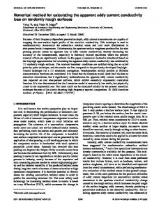
Modelling phase change materials There are several issues to consider when modelling PCM in a whole-building simulation program. The main concern is the heat capacity's dependency on temperature including the effect of the hysteresis. Previous investigations (Kuznik and Virgone, 2008) have shown that it is important to take into account the hysteresis to obtain the correct heat transfer. Another issue is the temperature dependency of the thermal conductivity. Here previous investigations (Hoffmann and Kornadt, 2006), (Heim and Clarke, 2003) and (Kuznik et al, 2008) have pointed out that the temperature dependency of the thermal conductivity of the PCM is also relevant to include in the model. The method used for performing PCM calculations in BSim is best described through an example; The Micronal SmartBoard (30%, 23°C) is a building material containing PCM. The SmartBoard is a 15 mm thick gypsum board containing 30% (3 kg pr. m2) of microencapsulated PCM (paraffin). The board has a specific heat capacity of 1.20 kJ/kgK, a thermal conductivity of 0.18 W/mK (in solid state) and a latent heat capacity in the transition area of 330 kJ/m2. In figure 2 the enthalpy is shown as a function of temperature.
(2)
By expressing the specific enthalpy change as a temperature change multiplied by the specific heat capacity and by inserting the expressions for q from (1), the following equation is obtained:
Ti j +1 − Ti j = p i i Δt Ti −j1+1 − Ti j +1 Ti +j1+1 − Ti j +1 + Δxi −1 Δxi Δxi Δxi +1 + + Ri + + Ri +1 2λi −1 2λi 2λi 2λi +1
(4)
Initially all temperatures in the equation system is set to a fixed temperature (standard is 20 °C), and from these starting values the first day of the simulation period is repeated several times until stability has been obtained, e.g. a steady circadian rhythm or a quasi-steady-state.
(ρc ) Δx
80000 70000 60000 Enthalpy [J/kg]
1
conditions are known, which is why equation (3) for the boundary control volume ("i"=1) becomes:
50000 Melting Solidifying
40000 30000 20000 10000
(3)
0 0
5
10
15
20
25
30
35
Temperature [C]
Figure 2 Enthalpy as a function of temperature
This equation is constructed for all "i" and solved simultaneously. This is only possible if the boundary
- 401 -
In order to model the hysteresis we need to have information about the PCM state at the previous time-step in order to calculate the state of the present time-step, i.e. the state at any time is path-dependant. We have chosen to use a simplified method for taking into account the effect of the hysteresis. For a phase change material the heat capacity for control volume "i" in time-step "j" is based on the temperature of the control volume in time-step "j-1", i.e. the last known temperature of the control volume. Using this simplified approach we avoid adding unneccesary complexity to the simulation model. However, it requires that time-steps are so small that instability of the calculation is avoided. As mentioned earlier, before the actual simulation begins the temperature is 20°C throughout the model and for any PCM in the model we define this initial state as being "on the melting curve". Hereafter, the state will always follow either the melting curve (heating), the solidifying curve (cooling), or be somewhere between the curves. Between the curves the state will move horizontally until it reaches either the melting or the solidifying curve. The method is visualised in figure 3 where arrows symbolise the transition of the PCM state.
Figure 4 Experimental setup. 18 SmartBoards bolted together and surrounded by insulation. Test A In the first test steady-state conditions prevail when a 1000W lamp is lit on one side of the wall. The lamp can increase the surface temperature to just above 60°C. In figure 5 the node temperatures (boundary nodes plus one for every third board) are shown as a function of time. The thick lines are measurements while thin lines are calculations. Temperature measurements on either side of the wall are used as boundary conditions in simulations.
60000 55000
Enthalpy [J/kg]
50000 45000
Melting Solidifying
40000 35000 30000 25000 18
19
20
21
22
23
Temperature [C]
Figure 3 State of PCM. Sample melt/solidify loop
Figure 5 Test A. Continuous heating.
When the state is between the melting and solidifying curves, the total heat capacity is found through linear interpolation between the corresponding points on the melting and solidifying curve.
From figure 5 it is evident that the temperature profiles show the same tendencies. Melting generally occurs later in the simulation model than in measurements, i.e. 15 mm inside the construction there is a delay of 15 minutes and the further into the construction the longer the delay. 60 mm inside the construction the delay is 2 hours. This could either indicate that the latent heat is too low in the calculation model or that the thermal conductivity is higher than expected.
VALIDATION Validation was performed for a relatively simple setup, and further validation will be carried out as soon as more measurements become available. The background for the validation is laboratory measurements (Pedersen, 2008) on a 270 mm thick "wall" of Micronal SmartBoards, i.e. 18 boards of 15 mm thickness bolted together. Figure 4 shows the experimental setup.
Test B Test B is similar to test A, however after 20 hours the lamp is shut off and cooling is initiated. Figure 6 shows temperature as a function of time for both measurement (thick lines) and simulation (thin lines).
- 402 -
Figure 8 Test C. Continuous heating.
Figure 6 Test B. 20 hours heating then cooling. Figure 6 shows a reasonably good agreement between measurement and simulation, however it seems that there is a general shifting of the temperatures, i.e. approximately 2°C for the node closest to the warm side. This may be due to the surface temperature measurement being influenced by the radiation from the lamp. A second calculation is performed where node 2 is used as boundary condition instead. Results are shown in figure 7.
Figure 9 Test C. Phase change close-up. The overall conclusions from comparing measurements and simulations are; the simulation model seems to work in general and deviations are fairly small. If we leave out the surface temperature from the measurements, the overall agreement is good and it is clear that only minor differences are present.
CALCULATION EXAMPLES Figure 7 Test B. Node 2 as boundary condition. Figure 7 shows that using the temperature at node 2 results a in much better agreement between measurements and simulation, and therefore it is concluded that the measurement of the surface temperature is to some extent flawed. Test C Test C is identical to test A except that the initial temperature is below the melting point of the PCM. Figure 8 shows temperatures for both measurements and simulation. In the simulation node temperature 2 is used as boundary condition. Figure 8 shows a relatively good agreement between measurements and simulation. Again, the further into the construction the larger the errors which could indicate that the melting heat is too low. Figure 9 shows a close-up of the temperatures in the phase change area, and these indicate that the simulation model is not sufficiently dynamic to model the PCM.
A few simple calculations have been performed in order to evaluate the PCM module. The model used for these calculations is a simple two-room model. The rooms are geometrically identical. One room is a reference room and the other room is for testing different constellations of PCM usage.
Figure 10 Simple BSim model Each office has a depth of 5.0 m, a width of 4.0 m and a height of 2.8 m. Both offices have a window
- 403 -
1.0 m high and 2.0 m wide facing south. All constructions in the model are light constructions with 225 mm insulation bounded by 16 mm plywood on both sides. The offices have identical systems. The internal heat load is 100 W. The heating system has a maximum effect of 100 kW and a setpoint of 20.1°C. The cooling system has a maximum effect of 100 kW and a setpoint of 24.0°C. Yearly simulations are performed using weather data for the Danish design year, DRY (Jensen and Lund, 1995). The heating and cooling demand for the reference office is 361 kWh and 361 kWh respectively. PCM area The first analysis is an investigation of how much PCM that can be utilised in the room, and whether there is an upper limit to how much that can be added. The plywood on the inside of the constructions are substituted by the SmartBoard described earlier. In the first simulation we replace the plywood in the ceiling with the SmartBoard, in the second we also replace the plywood on one wall and so forth. In the last simulation all plywood have been replaced by SmartBoard, except for the partitioning wall between the two offices. In figure 11 the energy use for heating and cooling is shown as a function of the total area of PCM.
Difference in heating/cooling demand [kWh]
14 12 10 Heating Cooling
8 6 4 2 0 Jan Feb Mar Apr May Jun
Jul Aug Sep Oct Nov Dec
Figure 12 Difference in heating and cooling demand between model with and without PCM Figure 12 shows that the difference in the heating and cooling demand between the two offices, is larger in spring and autumn than during winter and summer. The reason for this is that the room temperature during winter is low (close to 20°C) for both offices and therefore the PCM is not activated, and during summer it is the opposite situation, where the temperature is high throughout the day, meaning that the PCM does not get to discharge the stored heat. This clearly shows that the utilisation of PCM in buildings is only efficient if the temperature fluctuations during a day are so that the PCM is first melted and then solidified, otherwise it is not possible to take advantage of the materials properties.
CASE STUDY
400
A case study is performed with BSim on a small twostorey house located on the platform roof of an existing building.
375 Energy use [kWh]
16
350 Heating Cooling
325 300 275 250 0
20
40
60
80
Area of PCM [m2]
Figure 11 Energy use as a function of PCM area The figure clearly shows that the relative effect of the PCM is reduced when the area is increased. The first 20 m2 decreases the energy use significantly whereas the last 20 m2 give almost no reduction. This is what we would expect, i.e. that there is an upper limit to the amount of PCM that can be utilised. PCM seasonal variations If we take a closer look at the simulation results for the situation with 16 mm PCM on the ceiling, and examine how the heating and cooling demand varies over the year, we get graphs as shown in figure 12.
Figure 13 Section of the dwelling house The house is 9.25 m in length and 4.20 m in width. The effective area is about 60 m² and the volume is about 220 m³. The roof and walls are light-weight constructions so that there is only a small thermal mass for heat storage. The building is highly insulated. The U value of the roof is 0.155 W/m²K. To the left and to the right of the building are similar buildings. This means that there is no heat loss through the eastern and western walls. As a buffer zone a winter garden is placed in the south end of the building. Heating is done by the ventilation system. The building is located in Munich, Germany.
- 404 -
Figure 16 represents the total heat load for every hour of the year in the thermal zone ‘dwelling’. One can even see the heat coming from cooking at 12:00 o’clock and 18:00 o’clock. a[0..0,1]
b[0,1..10]
c[10..20]
d[20..30]
e[30..40]
f[40..50]
g[50..60]
h[60..70]
i[-]
Tageszeit [h]
24 18 12 6 0 0
Jan30
Feb60
Mrz 90
Apr 120 Mai 150 Jun 180 Jul 210Aug 240Sep 270Okt
300 Nov
330 Dez
360
Figure 16 Total heat load [W/m²] during the year
The task formulation for the simulation with BSim is the optimization of thermal room climate by the use of PCM. For the simulation the building is constructed as a model with four thermal zones (dwelling, bathroom, winter garden, and entrance). The data of TRY 13 are used as climate file.
For the documentation of the simulation results the analysis of the zone ‘dwelling’ is shown for both variations: a[16,6..20]
b[20..22]
c[22..24]
d[24..26]
e[26..28]
f[28..30]
g[30..32]
h[32..35]
i[-]
24 T ag esz eit [ h ]
Figure 14 BSim model
18 12 6 0 0
Jan30
Feb60
Mrz 90
Apr 120 Mai 150 Jun 180 Jul 210Aug 240Sep
270Okt
300Nov
330 Dez
360
Figure 17 Hourly room temperature [°C] within a year for the variation ‘Basis’ a[16,9..20]
b[20..22]
c[22..24]
d[24..26]
e[26..28]
f[28..30]
g[30..32]
h[32..35]
i[-]
Tageszeit [h]
24 18 12 6 0 0
Jan30
Feb60
Mrz 90
Apr 120 Mai 150 Jun 180 Jul 210Aug 240Sep 270Okt
300 Nov
330 Dez
360
Figure 18 Hourly room temperature [°C] within a year for the variation ‘PCM’
Simulations for two variations are carried out: Variation 1 is the “Basis”, representing the initial state as reference building. It is built without PCM. For night cooling, the air change rate is allowed to reach 5/h with a set temperature of 20.5°C. The time profile for night cooling is restricted to the summer months. Variation 2 is named “PCM”. Micronal Smartboard with a thickness of 15 mm is installed in the sheathing at the bottom side of the roof. For the night cooling with a maximum of 5/h the ventilation has also got the set temperature of 20.5°C and the same time profile ‘summer’. The heat sources are the same in both variations. The total heat load is the sum of heat load through people, equipment, lighting, and solar gains, see table 1.
The carpet presentations above show the room temperature for each of the 8760 hours in a year assigned to the daytime [h] (Y axis) and the days of the years (X axis). Figure 17 shows the room temperature for the thermal zone ‘dwelling’ for the ‘Basis’ without PCM. Figure 18 shows the room temperature for the thermal zone ‘dwelling’ for the variation ‘PCM’ with PCM in the roof. Compared to each other, one can see that the building with PCM has less high room temperatures during summer. In winter the room temperatures in both variations are very similar. The overheating rates (room temperatures above 26°C) are 0.6% for the variation ‘Basis’ and 0.2% for the variation ‘PCM’ of the operation time. The air change rate is nearly the same for both variations.
Table 1 Heat sources in BSim models
a[0,01..0,2]
Heat load
Total [W/m²]
30,9
Heat energy [kWh/m²a] 73,4
People Equipment
2,4 14,8
16,7 6,1
Lighting
7,0 15,1
c[1..2]
d[2..3]
e[3..4]
f[4..5]
g[-]
h[-]
i[5..5,7]
18 12 6 0 0
Zone
b[0,2..1]
24 Tageszeit [h]
Figure 15 VRML presentation showing the thermal zones of the BSim model (by the tool 3D ThermalView)
Solar
Jan30
Feb60
Mrz 90
Apr 120 Mai 150 Jun 180 Jul 210Aug 240Sep 270Okt
300 Nov
330 Dez
360
Figure 19 Hourly air change [1/h] within a year for the variation ‘PCM’
30,1 37,5
- 405 -
BSim also calculates the temperature distribution within the construction. The diagrams below show the temperatures within the building construction roof. Temperatures are presented for a cold winter day (February 16th, at 5:00, 12:00, 16:00 and 19:00 o’clock) and a hot summer day (August 1st, at 5:00, 12:00, 16:00 and 19:00 o’clock). Figure 20 represents the roof without PCM (with a clay board instead) for the variation ‘Basis’ and figure 21 shows the roof with PCM for the variation ‘PCM’.
Figure 23 Monthly heat balance for the thermal zone ‘dwelling’ (variation ‘PCM’) Differences appear mainly in the monthly energy for heating: The building without PCM (‘Basis’) needs more energy for heating in winter. Table 2 shows essential results of the variations ‘Basis’ and ‘PCM’ in comparison.
Figure 20 Temperature distribution in the roof with clay boards (variation ‘Basis’)
Table 2 Simulation results for ‘Basis’ and ‘PCM’ Name
Basis PCM
Zone
[>26°C] Max. Heating_total [h/a] [°C] [kWh/m²a]
Venting [kWh/m²a]
Dwelling
39
28,7
10,4
35,2
Dwelling
13
28,0
8,8
35,4
By the use of the PCM Micronal Smartboard in the roof of the building, the overheating frequency is reduced about a third. During a day when the PCM board is loaded, the room temperature is up to 2 K lower than without PCM. The heating energy demand is slightly lowered. The energy demand for venting against overheating stays nearly the same.
Figure 21 Temperature distribution in the roof with PCM boards (variation ‘PCM’) Noontime solar heating from outdoors does not reach the inner room. The temperature in the PCM board is constant throughout the day. On the summer day the temperature in the clay board is higher than in the PCM board. The indoor temperature is 2.1 K higher in the room with the clay board than in the room with the PCM board. Among other characteristics, also the heat balance for the variations is calculated.
Figure 22 Monthly heat balance for the thermal zone ‘dwelling’ (variation ‘Basis’)
DISCUSSION A PCM module have been added to BSim, and a simple validation process based on laboratory measurements have been carried out. This validation indicates that the module can predict PCM behaviour in building constructions with a good precision. Simple calculations indicate that there is an upper limit to the area of PCM that can be utilised in a room. The simple calculations demonstrate how the PCM module can be used for investigating different aspects of PCM behaviour. A case study where a PCM layer have been installed in a roof’s bottom side were also performed. This study shows that a building taking advantage of PCM has to have certain temperature fluctuations. The temperature fluctuation amplitude has to be high enough so that the PCM can work. It is useless to install PCM in a building with a very constant temperature level so that the PCM is never activated. For instance, on the solidifying curve between 20°C and 19°C, the PCM has about 20 % of its enthalpy (see figure 3). To discharge this energy it is necessary that the room temperature has to drop down to 19°C which is beneath the heating set point. These required temperature fluctuations have a nega-
- 406 -
tive impact on the dwelling comfort. Further, the fluctuations enforce their claims to system engineering. The systems have to be operated by demanding control strategies, especially for natural ventilation.
CONCLUSION A numerical method for calculating latent heat storage in constructions containing phase change material has been developed. The method has been implemented in BSim and has undergone a simple validation based on comparisons to laboratory measurements. This paper has also presented some simple calculation examples that demonstrates how the module works and how it can be utilised for theoretical analysis. Finally, a case study has presented an example showing how the module can be used for optimising indoor climate in a room using PCM.
FUTURE WORK Detailed measurements are presently being performed on a full-scale building containing PCM for further validation of the calculation model.
ACKNOWLEDGEMENTS This work was sponsored by the Danish Energy Association.
NOMENCLATURE q:
heat flux [W/m2]
Δx:
control volume width [m]
λ: R: i: j: h:
thermal conductivity [W/mK] thermal resistance [m2K/W] index for the place [-] index for the time [-] specific enthalpy [J/kg]
Δt: size of the time-step [s] qsurfside1: heat transfer directly to the surface [W/m2] Rsurfside1: thermal resistance for surface [m2K/W] ρ: cp:
density [kg/m3] heat capacity [J/kgK]
REFERENCES
Ibáñez, M., Lázaro, A., Zalba, B. and Cabeza, L.F. 2005. An approach to the simulation of PCMs in building applications using TRNSYS. Applied Thermal Engineering 25, pp. 1796-1807. Lomas, K.J., Eppel, H., Martin, C., Bloomfield, D. and Watson, M. 1994. Empirical validation of thermal building simulation programs using test room data. IEA Annex 21 / IEA SHC Task 12. Jensen, J. M. and Lund, H. 1995. Design reference year, DRY – Et nyt dansk referenceår. Meddelelse nr. 281. Laboratoriet for Varmeisolering, Danmarks Tekniske Universitet. Kuznik, F., Virgone, J. and Roux, J.J. Energetic efficiency of room wall containing PCM wallboard: A full-scale experimental investigation. Energy and Buildings, vol. 40, pp. 148-156. Kuznik, F. and Virgone, J. 2008. Experimental investigation of wallboard containing phase change material: Data for validation of numerical modeling. Energy and Buildings. Article in press (available online). Pedersen, C. O. 2007. Advanced zone simulation in Energyplus: Incorporation of variable properties and phase change material (PCM) capability. 10th International IBPSA Conference, Beijing, China. Pedersen, S. 2008. PCM, genvinding og fjernelse af varme via faseskiftende materialer. Bachelor Project from Engineering College of Aarhus. Stetiu, C. and Feustel, H.E. 1998. Phase-change wallboard and mechanical night ventilation in commercial buildings. Lawrence Berkeley National Laboratory, Berkeley, CA, USA. Stetiu, C., Feustel, H.E. and Winkelmann, F.C. 1995. Development of a model to simulate the performance of hydronic radiant cooling ceilings. ASHRAE Transactions 101 (2): 730743. Wittchen, K.B., Johnsen, K., Sørensen, K.G. and Rose, J. 2008. BSim User's Guide. Danish Building Research Institute, Aalborg University.
Heim, D. 2005. Two solution methods of heat transfer with phase change within whole building dynamic simulation. 9th International IBPSA Conference, Montréal, Canada. Heim, D. & Clarke, J.A. 2003. Numerical modelling and thermal simulation of phase change materials with ESP-r. 8th International IBPSA Conference, Eindhoven, Netherlands. Hoffmann, S. & Kornadt, O. 2006. An investigation on phase change materials to reduce summer overheating. IBPSA-Canada's 4th Biennial Building Performance Simulation Conference.
- 407 -