Numerical Modeling of Expansive Soil Behavior - UniversitÃ¤t Stuttgart

2008 - Mitteilung 56

Ayman Abed

Numerical Modeling of Expansive Soil Behavior Ayman Abed

2008 − Mitteilung 56 des Instituts für Geotechnik Herausgeber P. A. Vermeer

IGS

Numerical Modeling of Expansive Soil Behavior

Von der Fakultät für Bau– und Umweltingenieurwissenschaften der Universität Stuttgart zur Erlangung der Würde eines Doktors der Ingenieurwissenschaften (Dr.-Ing.) genehmigte Abhandlung,

vorgelegt von

AYMAN A. A BED aus Homs, Syrien

Hauptberichter:

Prof. Dr.-Ing. Pieter A. Vermeer

Mitberichter:

Prof. Antonio Gens

Tag der mündlichen Prüfung:

22. Februar 2008

Institut für Geotechnik der Universität Stuttgart 2008

Mitteilung 56 des Instituts für Geotechnik Universität Stuttgart, Germany, 2008

Editor: Prof. Dr.-Ing. P. A. Vermeer c Ayman Abed Institut für Geotechnik Universität Stuttgart Pfaffenwaldring 35 70569 Stuttgart All rights reserved. No part of this publication may be reproduced, stored in a retrieval system, or transmitted, in any form or by any means, electronic, mechanical, photocopying, recording, scanning or otherwise, without the permission in writing of the author. Keywords: Unsaturated soil, constitutive soil models Printed by e.kurz + co, Stuttgart, Germany, 2008 ISBN 978-3-921837-56-6 (D93 - Dissertation, Universität Stuttgart)

Preface Expansive soils contain clay minerals named montmorillonites or smectites. In this type of soils, significant deformations are associated with changes in suction and degree of saturation. As expansive soils are widespread in nature, they constitute an important challenge for geotechnical engineering. In the unsaturated zone well above the phreatic groundwater level the soil moisture content varies significantly over the seasons and the study of expansive soil behaviour is thus based on unsaturated soil mechanics and unsaturated groundwater flow. At present unsaturated flow is getting increasing attention in literature and so is the mechanical behaviour of unsaturated soils. Although the title of this study refers to expansive soils, most of the developments reported are applicable to unsaturated soils in general. Being from Syria, a land with large areas of expansive soils, Ayman Abed came to Stuttgart to study the mechanical behaviour of such soils. Being not a specialist in this field, I was very pleased to have my colleague Professor Antonio Gens from Barcelona as a co-advisor. No doubt, the Barcelona Basic Model represented the state-of-the-art in the elastoplastic modelling of unsaturated soils in the year 2004 when Ayman Abed came to Stuttgart, and a detailed description of this model is contained in the present study. The main original contribution of this thesis to geomechanics is the extension or generalisation of the Barcelona Basic Model from isotropic to anisotropic soil. Indeed unsaturated clays are mostly anisotropic and should thus be modelled within the framework of anisotropic plasticity as presently also done for saturated clays. This study represents a significant contribution to the subject of unsaturated soil mechanics that can be used as a spring board for further research in this challenging field of geomechanics. To me it has been a great pleasure to work with Ayman Abed and I am very happy to congratulate him with this achievement of the doctoral thesis. Pieter A. Vermeer Stuttgart, February 2008

Acknowledgments I am deeply indebted to my supervisor Professor Pieter A. Vermeer for his ultimate help, guidance and constructive criticisms. Working with Professor Vermeer is an event by itself. Beside scientific development, the daily discussion with Professor Vermeer enriched my personal knowledge in general. I am also very thankful to my co-advisor Prof. Antonio Gens for his critical comments. I learned a lot from him when discussing the unsaturated soil behavior. I wish to thank the Syrian government who has provided me with a very convenient four years scholarship which guaranteed a smooth completeness of my thesis. Special thank to the workers in the Syrian embassy and the Syrian students community in Berlin for their efforts to keep us focusing on our studies by solving all bureaucratic problems. I also wish to thank all my colleagues in the Institute of Geotechnical Engineering (IGS) for the pleasant time that I spent with them, I felt always as if I were with my family. Universität Stuttgart and in particular my doctoral program “ENWAT” are highly acknowledged for providing me with learning opportunities of very high standards. My thanks go to the following persons for the fruitful discussions about unsaturated soil behavior and the numerical implementation issues: Mr. John van Esch and Dr. Peter van den Berg from Geodelft, the Netherlands, Dr. Klaas Jan Bakker from Delft University, Dr. Paul Bonnier from Plaxis B.V. At the Institute of Geotechnical Engineering of Stuttgart University I very much enjoyed the discussion with my colleagues Dr. Jilin Qi, Dr. Martino Leoni, Dr. Thomas Benz, Josef Hintner, Axel Möllmann and Syawal Satibi. My deep thank is also due to our marvelous secretaries Ruth Rose and Nadja Springer for their ultimate help and care. I am most grateful to my family, without their love, care and continuous support this thesis would never be finished. Ayman A. Abed Stuttgart, February 2008

Dedicated to my brother Wael ... the man of honor ...

Contents 1 Introduction 1.1 Unsaturated expansive soil 1.2 Motivation . . . . . . . . . . 1.3 Surface tension and suction 1.4 Objectives and scope . . . . 1.5 Layout of Thesis . . . . . . .

. . . . .

1 1 2 3 4 4

. . . . . . .

7 7 7 11 13 16 19 20

. . . . . . . . . . . . . . . .

27 27 28 29 32 33 33 34 36 36 38 40 40 41 44 44 45

4 Elastoplastic Modeling of Unsaturated Soil 4.1 Introduction . . . . . . . . . . . . . . . . . . . . . . . . . . . . . . . . . . . .

47 47

. . . . .

. . . . .

. . . . .

. . . . .

. . . . .

. . . . .

. . . . .

. . . . .

. . . . .

. . . . .

. . . . .

. . . . .

. . . . .

. . . . .

. . . . .

. . . . .

. . . . .

. . . . .

. . . . .

. . . . .

. . . . .

. . . . .

. . . . .

. . . . .

. . . . .

2 Fundamental Principles 2.1 Sign convention . . . . . . . . . . . . . . . . . . . . . . . . . . . . . . . . 2.2 Stresses and equilibrium . . . . . . . . . . . . . . . . . . . . . . . . . . . 2.3 Displacements and strains . . . . . . . . . . . . . . . . . . . . . . . . . . 2.4 Stresses in unsaturated soil . . . . . . . . . . . . . . . . . . . . . . . . . 2.5 Stress-strain relationship for unsaturated elastic soil . . . . . . . . . . . 2.6 Experimental determination of elastic soil parameters . . . . . . . . . . 2.6.1 Typical stress paths as used in triaxial tests on unsaturated soil 3 Elastoplastic Modeling of Soil 3.1 Introduction . . . . . . . . . . . . . . . . . . . . . . . . . . . 3.2 Plastic behavior modeling . . . . . . . . . . . . . . . . . . . 3.2.1 Yield function . . . . . . . . . . . . . . . . . . . . . . 3.2.2 Flow rule . . . . . . . . . . . . . . . . . . . . . . . . . 3.2.3 Hardening law . . . . . . . . . . . . . . . . . . . . . 3.2.4 The consistency condition . . . . . . . . . . . . . . . 3.3 The stress-strain formulation in case of elastoplastic model 3.4 Cam Clay model . . . . . . . . . . . . . . . . . . . . . . . . 3.4.1 Isotropic loading . . . . . . . . . . . . . . . . . . . . 3.4.2 Yield surface and flow rule . . . . . . . . . . . . . . 3.4.3 Modified Cam Clay hardening rule . . . . . . . . . 3.4.4 Elastoplastic matrix for Cam Clay model . . . . . . 3.4.5 On the failure criterion as used in Cam Clay . . . . 3.5 On Modified Cam Clay parameters . . . . . . . . . . . . . . 3.5.1 Stiffness parameters as used in Cam Clay model . . 3.5.2 Strength parameter as used in Cam Clay model . .

. . . . . . . . . . . . . . . .

. . . . . . . . . . . . . . . .

. . . . . . . . . . . . . . . .

. . . . . . . . . . . . . . . .

. . . . . . . . . . . . . . . .

. . . . . . . . . . . . . . . .

. . . . . . . . . . . . . . . .

. . . . . . . . . . . . . . . . . . . . . . . . . . . .

i

Contents 4.2

4.3 4.4

4.5

Experimental evidences . . . . . . . . . . . . . . . . . . . . . 4.2.1 Effect of suction on soil stiffness . . . . . . . . . . . . 4.2.1.1 Loading-unloading under constant suction 4.2.1.2 Wetting under constant net stress . . . . . . 4.2.1.3 Drying under constant net stress . . . . . . . 4.2.1.4 Yielding of unsaturated soil . . . . . . . . . 4.2.2 Effect of suction on soil strength . . . . . . . . . . . . 4.2.3 Summary on the experimental observations . . . . . Early attempts to model unsaturated soil behavior . . . . . . 4.3.1 Volumetric and shear strains . . . . . . . . . . . . . . 4.3.2 Shear strength . . . . . . . . . . . . . . . . . . . . . . . Barcelona Basic Model . . . . . . . . . . . . . . . . . . . . . . 4.4.1 Isotropic loading . . . . . . . . . . . . . . . . . . . . . 4.4.1.1 Net stress primary loading-unloading . . . 4.4.1.2 Suction primary loading-unloading . . . . . 4.4.1.3 General expression for isotropic stress state 4.4.1.4 Isotropic plastic compression upon wetting 4.4.2 More general states of stress . . . . . . . . . . . . . . . 4.4.2.1 Elastic behavior . . . . . . . . . . . . . . . . 4.4.2.2 Plastic behavior . . . . . . . . . . . . . . . . 4.4.2.3 LC and SI coupling . . . . . . . . . . . . . . 4.4.3 Elastoplastic matrix for Barcelona Basic Model . . . . On the parameters of Barcelona Basic Model . . . . . . . . . 4.5.1 Parameters β, λ∞ and pc . . . . . . . . . . . . . . . . . 4.5.2 Suction stiffness parameters . . . . . . . . . . . . . . . 4.5.3 Capillary cohesion parameter . . . . . . . . . . . . . .

5 Finite Element Implementation 5.1 Introduction . . . . . . . . . . . . . . . . . . . . . . . . . . 5.2 Balance and kinematic equations . . . . . . . . . . . . . . 5.3 Virtual work principle . . . . . . . . . . . . . . . . . . . . 5.4 Finite element discretization in case of unsaturated soil . 5.5 Local integration of constitutive equation . . . . . . . . . 5.5.1 Explicit integration . . . . . . . . . . . . . . . . . . 5.5.2 Implicit integration . . . . . . . . . . . . . . . . . 5.5.2.1 Elastic predictor . . . . . . . . . . . . . . 5.5.2.2 Plastic corrector with return mapping . . 5.5.3 Stress integration with LC is active . . . . . . . . . 5.5.4 Stress integration with SI is active . . . . . . . . . 5.5.5 Stress integration when both LC and SI are active 5.6 The global iterative procedure . . . . . . . . . . . . . . . . 5.6.1 Global and element stiffness matrices . . . . . . . 5.6.2 Global Newton-Raphson iterations . . . . . . . . . 5.7 Validation of the BB-model implementation . . . . . . . .

ii

. . . . . . . . . . . . . . . .

. . . . . . . . . . . . . . . .

. . . . . . . . . . . . . . . . . . . . . . . . . . . . . . . . . . . . . . . . . .

. . . . . . . . . . . . . . . . . . . . . . . . . . . . . . . . . . . . . . . . . .

. . . . . . . . . . . . . . . . . . . . . . . . . . . . . . . . . . . . . . . . . .

. . . . . . . . . . . . . . . . . . . . . . . . . . . . . . . . . . . . . . . . . .

. . . . . . . . . . . . . . . . . . . . . . . . . . . . . . . . . . . . . . . . . .

. . . . . . . . . . . . . . . . . . . . . . . . . . . . . . . . . . . . . . . . . .

. . . . . . . . . . . . . . . . . . . . . . . . . . . . . . . . . . . . . . . . . .

. . . . . . . . . . . . . . . . . . . . . . . . . .

47 47 48 49 51 52 52 54 55 55 57 60 60 61 62 63 64 66 66 67 69 69 73 73 75 75

. . . . . . . . . . . . . . . .

77 77 78 79 80 83 83 84 84 84 87 87 89 91 91 92 94

Contents 5.7.1 5.7.2 5.7.3 5.7.4 5.7.5 5.7.6

Test Number 1 . Test Number 2 . Test Number 3 . Test Number 4 . Test Number 5 . Test Number 6 .

. . . . . .

. . . . . .

. . . . . .

. . . . . .

. . . . . .

. . . . . .

. . . . . .

. . . . . .

. . . . . .

. . . . . .

. . . . . .

. . . . . .

. . . . . .

. . . . . .

. . . . . .

. . . . . .

. . . . . .

. . . . . .

. . . . . .

. . . . . .

. . . . . .

. . . . . .

. . . . . .

. . . . . .

. . . . . .

. . . . . .

. . . . . .

. . . . . .

. . . . . .

. 95 . 97 . 98 . 98 . 102 . 102

6 Unsaturated ground water flow 6.1 Introduction . . . . . . . . . . . . . . . . . . . . . . . . . . . . . . . . . . 6.2 Governing partial differential equation . . . . . . . . . . . . . . . . . . . 6.2.1 Steady-state water flow . . . . . . . . . . . . . . . . . . . . . . . 6.2.2 Transient saturated water flow . . . . . . . . . . . . . . . . . . . 6.2.3 Transient unsaturated water flow . . . . . . . . . . . . . . . . . . 6.2.4 Multiphase flow . . . . . . . . . . . . . . . . . . . . . . . . . . . 6.2.5 Fitting functions for soil degree of saturation . . . . . . . . . . . 6.2.6 Fitting functions for soil water permeability . . . . . . . . . . . 6.3 Finite element discretization in space . . . . . . . . . . . . . . . . . . . . 6.4 Finite differences discretization in time . . . . . . . . . . . . . . . . . . . 6.5 Picard iteration method . . . . . . . . . . . . . . . . . . . . . . . . . . . 6.6 Validation of the finite element code being used . . . . . . . . . . . . . 6.6.1 Validation in case of unsaturated stationary ground water flow 6.6.2 Validation in case of unsaturated transient ground water flow .

. . . . . . . . . . . . . .

. . . . . . . . . . . . . .

105 105 105 105 106 109 109 112 114 116 117 118 119 119 121

7 Anisotropic model for unsaturated soil 7.1 Introduction . . . . . . . . . . . . . . . . . . . . . . . . . . . . . . . . . . . . 7.2 Origin of anisotropy . . . . . . . . . . . . . . . . . . . . . . . . . . . . . . . 7.3 Empirical observations and constitutive modeling of anisotropy . . . . . . 7.4 Models based on Cam Clay model . . . . . . . . . . . . . . . . . . . . . . . 7.4.1 SANICLAY model . . . . . . . . . . . . . . . . . . . . . . . . . . . . 7.4.2 S-Clay1 model for anisotropic soil . . . . . . . . . . . . . . . . . . . 7.4.2.1 The initial value of α . . . . . . . . . . . . . . . . . . . . . 7.4.2.2 The constant β . . . . . . . . . . . . . . . . . . . . . . . . . 7.4.2.3 The constant µ . . . . . . . . . . . . . . . . . . . . . . . . . 7.4.2.4 S-Clay1 in the general state of stress . . . . . . . . . . . . . 7.5 Anisotropy in unsaturated soil . . . . . . . . . . . . . . . . . . . . . . . . . 7.5.1 Anisotropic model for unsaturated soil . . . . . . . . . . . . . . . . 7.5.1.1 Flow and hardening rules . . . . . . . . . . . . . . . . . . 7.5.1.2 General states of stress . . . . . . . . . . . . . . . . . . . . 7.5.1.3 Numerical implementation of the new anisotropic model 7.6 Numerical validation of the implemented model . . . . . . . . . . . . . . . 7.6.1 Case 1: Isotropic fully saturated soil . . . . . . . . . . . . . . . . . . 7.6.2 Case 2: Isotropic unsaturated soil . . . . . . . . . . . . . . . . . . . . 7.6.3 Case 3: Anisotropic fully saturated soil . . . . . . . . . . . . . . . .

123 123 123 124 125 125 128 129 129 130 130 131 133 135 136 137 138 140 142 144

iii

Contents 8 Boundary value problems 8.1 Introduction . . . . . . . . . . . . . . . . . . . . . . . . . . . . . . . . . . . . 8.2 Problem 1: Shallow foundation exposed to a ground water table increase . 8.2.1 Geometry, boundary conditions and initial conditions . . . . . . . . 8.2.2 The interaction between the ground water flow finite element code and the deformation code . . . . . . . . . . . . . . . . . . . . . . . . 8.2.3 Results of numerical analyses with isotropic BB-model . . . . . . . 8.2.4 Calculation with an anisotropic model . . . . . . . . . . . . . . . . . 8.3 Problem 2: Bearing capacity of unsaturated soil . . . . . . . . . . . . . . . . 8.4 Problem 3: Shallow foundation exposed to a rainfall event . . . . . . . . . 8.4.1 Phase 1: Deformation due to foundation loading . . . . . . . . . . . 8.4.2 Phase 2: Deformation due to infiltration . . . . . . . . . . . . . . . . 8.5 Problem 4: Trial wall on expansive soil in Sudan . . . . . . . . . . . . . . . 8.5.1 Soil properties . . . . . . . . . . . . . . . . . . . . . . . . . . . . . . 8.5.2 The test procedure and measurements . . . . . . . . . . . . . . . . . 8.5.3 Numerical simulation . . . . . . . . . . . . . . . . . . . . . . . . . . 8.5.3.1 Geometry and boundary conditions . . . . . . . . . . . . 8.5.3.2 Parametric study . . . . . . . . . . . . . . . . . . . . . . . 8.5.3.3 Model predictions versus field data . . . . . . . . . . . .

147 147 147 147

9 Conclusions and recommendations 9.1 Conclusions on modeling and numerical implementation . . . . . . . . . 9.2 Conclusions on the response of shallow foundation on unsaturated soil . 9.2.1 Isotropic behavior . . . . . . . . . . . . . . . . . . . . . . . . . . . 9.2.2 Anisotropic behavior . . . . . . . . . . . . . . . . . . . . . . . . . . 9.3 Recommendation for further research . . . . . . . . . . . . . . . . . . . .

175 175 176 176 176 177

Bibliography

iv

. . . . .

148 149 152 153 158 159 160 162 162 165 166 166 167 170

177

Abstract The mechanical behavior of unsaturated soils is one of the challenging topics in the field of geotechnical engineering. The use of finite element technique is considered as a promising method to solve settlement and heave problems, as associated with unsaturated soil. Nevertheless, the success of the numerical analysis is strongly dependent on constitutive model being used. Furthermore, solving unsaturated soil problems needs the assessment of suction variation in time and space as a response to the variation of environmental factors such as rainfall and evaporation rate. The well-known Barcelona Basic model (Alonso et al., 1990) is considered to be a robust and suitable model for the mechanical behavior of unsaturated soils and has thus been implemented into a finite element code. The so-called Richard’s equation is solved to determine suction field as associated with different initial and boundary conditions. Soil anisotropy is considered as well through the development and the implementation of a new anisotropic model for unsaturated soil. In addition to suction effects, this new model considers size and rotational hardening to capture anisotropy. This thesis begins with fundamental issues such as the definition of stress, strain, the effective stress concept and elasticity in unsaturated soil. Subsequently, the basics of elastoplasticity as used in the so-called critical state soil mechanics are reviewed placing emphasis on the Cam Clay model as an example for an elastoplastic soil model. The most important experimental observations concerning unsaturated soil mechanical behavior are also reviewed. The Cam Clay model is then extended in order to consider unsaturated states, yielding the Barcelona Basic model. The extension goes further by including the effect of anisotropy on soil response. In a special chapter, flow equations as used in solving suction variations in time and space are illustrated and discussed in details. After the theoretical development, the soil models are implemented into a finite element code and then employed to analyze some boundary value problems. The analyses include the study of soil plastic compression upon wetting and the simulation of soil swelling and shrinkage.

v

Abstract

vi

Zusammenfassung Das mechanische Verhalten von ungesättigten Böden ist eines der faszinierendsten Themenstellungen auf dem Gebiet der Geotechnik. Der Einsatz der Finite-Elemente-Methode wird als vielversprechend betrachtet, um Problemstellungen wie Setzungen und Hebungen, die mit ungesättigten Böden einhergehen, zu lösen. Nichtsdestotrotz ist der Erfolg der numerischen Analyse stark abhängig vom verwendeten Bodenmodell. Außerdem wird zur Lösung von Fragestellungen mit ungesättigten Böden die Abschätzung der Saugspannungen als Funktion der Zeit und des Ortes als Reaktion auf die Änderung von Umwelteinflüssen wie die Niederschlags- und die Evaporationsrate benötigt. Zur Bestimmung der Saugspannungen wird die bekannte Gleichung nach Richard herangezogen. Das Barcelona-Basic-Modell (BB-Modell) wird zur Modellierung der Auswirkung der Saugspannungen auf das mechanische Verhalten von ungesättigten isotropen Böden herangezogen und in ein Finite-Elemente-Programm implementiert. Zur Beschreibung der Eigenschaften von ungesättigten anisotropen Böden wird das BB-Modell erweitert und ebenfalls in ein Finite-Elemente-Programm implementiert. Die vorliegende Arbeit gliedert sich wie folgt: Kapitel 2 beinhaltet die Definitionen der Spannungen und der Dehnungen. Es zeigt auch die Elastizitätsgleichungen im Falle von ungesättigten Böden und die experimentelle Bestimmung der mechanischen Parameter von ungesättigten Boden. Kapitel 3 gibt einen Überblick über die grundsätzlichen Ideen der Elastoplastizität in der Bodenmechanik mit Berücksichtigung der Fließfunktion, der Konsistenzbedingung, der Fließregel, des Verfestigungsgesetzes und der elastoplastischen Steifigkeitsmatix. Das modifizierte Cam-Clay-Modell wird als Einführungsbeispiel verwendet, um die oben genannten Elemente zu erklären. Kapitel 4 erweitert die elastoplastische Formulierung auf ungesättigte Böden. Hierbei wird das “Barcelona-Basic-Model” verwendet, welches ein Vertreter von konstitutiven Modellen für ungesättigte Böden ist. Die Erweiterung wird durch experimentelle Beobachtungen unterstützt. Kapitel 5 gibt einen Überblick über die Grundlagen der Finite Elemente Methode für ungesättigte Böden. Dieses Kapitel beinhaltet die Implementierung des “BarcelonaBasic-Models” in einen Finite-Elemente-Code. Anschließend wird die Implementierung anhand von numerischen Elementversuchen validiert. Kapitel 6 behandelt die Grundwasserströmungs-Gleichung, die verwendet wird, um die Variation der Saugspannungen in Abhängigkeit von der Zeit zu bestimmen.

vii

Zusammenfassung In Kapitel 7 wird ein neues anisotropisches Stoffmodell für ungesättigte Böden vorgestellt, welches zusätzlich zu einer “size hardening” Regel eine “rotational hardening” Regel enthält. In diesem Kapitel werden ferner die Implementierung des Modells in einen Finite Element Code sowie dessen Validierung anhand exemplarischer Berechnungen behandelt. In Kapitel 8 werden Randwertsprobleme anhand der implementierten isotropischen und anisotropischen Stoffmodell diskutiert. Schwerpunkt liegt hierbei in der Betrachtung des Verhaltens einer Flachgründung bei Reduzierung und Erhöhung der Saugspannungen sowie bei Belastung des Untergrunds bis zum Versagen. Außerdem wird die Auswirkung der Anisotropie ungesättigter Böden auf das Verhalten des Untergrundes behandelt. Kapitel 9 enthält die Schlussfolgerungen dieser Dissertation und Vorschläge zu weiterführenden Forschungstätigkeiten.

viii

Chapter 1 Introduction 1.1 Unsaturated expansive soil Natural soils are often humid implying the existence of multiple phases in the soil pore space. In geotechnical applications, they are water and air. The expression unsaturated soil is used to refer to such a state of the soil. The fully saturated soil is a special case with water filling the entire soil pores. The ratio between the pore volume occupied by water and that occupied by air determines the so-called degree of soil saturation. The degree of saturation varies with time and is dependent on environmental factors such as temperature, rainfall, and ground water flow. From a mechanical point of view, a varying degree of saturation results in soil volume change which is relatively small in magnitude. However, for particular types of montmorillonite rich soils the volumetric change is of a considerable order. These soils are called expansive soils. The main reason for this phenomenon is the large specific surface1 of the (flaky) soil particles which enables the porous media to either suck in or lose a large amount of water during hydration or dehydration process. For shallow foundations soil shrinkage and soil swelling may cause considerable problems. Many financial loses are reported in literature due to the lack of correct understanding of the behavior of expansive soils in foundation engineering. To close the knowledge gap in this field, serious research on this topic began in the middle of 1960s. Since then, seven conferences under the name ’International Conference on Expansive Soils’ took place in 1965, 1969, 1973, 1980, 1984, 1987 and 1992. These conferences founded the so-called ’unsaturated soil mechanics’ as an independent science with extended rules as compared to classical soil mechanics. Later, four additional international conferences were held under the name ’Unsaturated Soil’; in 1995, 1998, 2002 and 2006. Today, studying the expansive soil behavior can not be separated from studying unsaturated soil mechanics.

1

the specific surface = the surface area of an individual soil particle / its volume or weight.

1

Chapter 1 Introduction

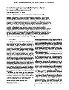
1.2 Motivation Expansive soil covers about 10% of the total area of Syria as can be seen in Figure 1.1. Up to now, only limited research efforts have been undertaken to solve foundation problems related to expansive soils even though this potentially problematic soil is abundant throughout the country. The problem extents to many other countries of the world like Canada, the United States, Australia, China, Spain, India, South Africa, Sudan, Ethiopia and Russia (Fredlund and Rahardjo, 1993).

med

iterra

nean

sea

For construction on expansive soil, pile foundations may be preferred, but they are often too costly for low-rise buildings. Therefore heave and settlement of shallow foundations on expansive clays will have to be studied in full detail. It is very common to use classical methods, neglecting any effect of the degree of saturation, to design such type of foundations. Even in the case of recognition of the expansive potential of the studied soil, crude empirical correlation tend to be used to estimated the amount of possible heave or plastic compression. These correlations relate the deformation to elementary soil index properties such as Plasticity Index Ip , Liquid Index wl or the clay content. It is believed that such empirical correlations give only satisfactory results as long as they are applied to the same soils which were used to derive them. This reduces their use to a very narrow group of soils. For a full revision of these methods the book by Nelson and Miller (1992) is recommended. In contrast, this dissertation uses the unsaturated soil mechanics principles to develop a suitable method to predict the deformation of a shallow foundation supported by an unsaturated expansive soil.

expansive soil sand saline soil gravel with a high organic content organic soil clay

Figure 1.1: Expansive soil distribution in Syria after Abed (2003).

2

1.3 Surface tension and suction

1.3 Surface tension and suction The so-called soil suction plays a major role in the mechanical response of unsaturated soil. It develops at the interface of two different soil phases. A water molecule inside the water is in balance as it is exposed to equal forces in all directions. However, a water molecule at the interface air-water experiences an unbalanced force towards the interior of the water as can be seen in Figure 1.2. This leads to a tensile pull along the interface, this pull is known as the surface tension. The surface tension causes the air-water interface to behave like a membrane. This membrane is subjected to different pressures on each side. Therefore, it shows a concave curvature towards the larger pressure and exerts a tension in the membrane in order to be in equilibrium. By the help of Figure 1.3 and using the balance equations, the pressure difference ∆u across the curved surface can be related to the surface tension Ts and the radius of curvature Rs as: ∆u =

2 · Ts Rs

(1.1)

In an unsaturated soil, the interface would be subjected to an air pressure ua greater than the water pressure uw . The pressure difference ∆u = ua − uw is referred to as matric suction s. Substitution of ∆u = ua −uw in Equation 1.1 gives the so-called Kelvin’s capillary model equation (Fredlund and Rahardjo, 1993): (ua − uw ) =

2 · Ts Rs

(1.2)

The above equation suggests that: • a decrease in the the radius of curvature implies an increase of suction. This case corresponds to the drying of soil where water retreats to smaller and smaller pores.

Molecule at the air-water interface

Molecule in the interior water

Figure 1.2: Intermolecular forces on a water molecule after Fredlund and Rahardjo (1993).

3


Ts

Rs

β β

β

Ts

Rs β

u+∆u

interface

u

Figure 1.3: Pressures and surface tension acting on a curved interface after Fredlund and Rahardjo (1993). • an increase of the radius of curvature implies a decrease of suction. This case corresponds to the wetting of soil where water penetrates into larger pores. A soil with high suction has a high potential to pull water into the soil matrix and vice versa. The surface tension Ts is a temperature dependent constant of the air-water interface. Furthermore, it is dependent on the chemical composition of the water. The variation in water chemistry introduces another suction component known as the osmotic suction. Throughout this report the word suction is used to indicate the matric suction only, neglecting any effect of temperature or osmotic suction on the mechanical behavior.

1.4 Objectives and scope The aim of this research is to model the behavior of expansive soil in the framework of unsaturated soil mechanics. The proposed model is used then to predict the displacements associated with the changes in soil suction. The final focus is on response of shallow foundations. However, the scope of application could be easily extended to other important problems such as slope stability. The finite element method is used to solve the governing partial differential equations. The elastoplasticity framework is used for constitutive modeling.

1.5 Layout of Thesis In addition to this introduction, the thesis is arranged in 8 chapters as indicated below: Chapter 2 includes the basic assumptions concerning the stress measures and the strain definition. It also illustrates the elasticity equations in case of unsaturated soils

4

1.5 Layout of Thesis with the required experimental techniques to determine the soil mechanical parameters. Chapter 3 reviews the fundamental ideas of soil elastoplasticity including the meaning of a yield function, a plastic potential function, a flow rule, a hardening rule and an elastoplastic stiffness matrix. The Modified Cam Clay Model is used as an introductory example to explain the above mentioned concepts. Chapter 4 extends the elastoplastic formulation to the case of unsaturated soil. The extension is supported by experimental observations. The Barcelona Basic Model is used as an example for a constitutive model of unsaturated soil. Chapter 5 reviews the basics of the finite element method as applied to unsaturated soil. This chapter includes the full implementation of the isotropic Barcelona Basic Model into a finite element code. It ends with numerical examples to validate the implementation. Chapter 6 introduces the flow equation used to solve the variation of suction over time. Finally the so-called Richard’s equation is introduced. The Soil Water Characteristic Curve and the relative permeability function are also discussed in this chapter. Chapter 7 introduces a new anisotropic model for unsaturated soil. The new model includes a rotational hardening law in addition to a size hardening rule. The implementation into a finite element code is discussed in full detail together with validation examples. Chapter 8 uses the implemented isotropic and anisotropic models to solve realistic boundary value problems. It focuses on shallow foundation response to suction reduction, suction increase and loading the soil up to failure. It also discusses the effect of unsaturated soil anisotropy on its behavior. Chapter 9 includes the conclusions of this research and the proposals for further developments.

5


6

Chapter 2 Fundamental Principles 2.1 Sign convention This section discusses the stress concept based on continuum mechanics principles. Compressive stresses and strains are considered to be positive for all cases, so that the sign convention is in accordance with that being used in soil mechanics literature.

2.2 Stresses and equilibrium Figure 2.1a illustrates the basic idea of mechanical equilibrium. If a body is in equilib-

Mz

external forces

Fz

Mx Fx Fy

My

δA z y x

external forces (a)

Figure 2.1: (a) External forces

(b)

(b) Including internal forces.

7

Chapter 2 Fundamental Principles

σyy τyx

τxz

τzx

y

σzz z

σ3

τyz

τxy

τzy

σ2

3

σxx

2

x

σ1

1 principal directions

(a)

(b)

Figure 2.2: Stress components.

rium, six equilibrium equations can be formulated. These equations relate the external forces affecting the body to one another. Three equations show that the sum of all forces acting in the three orthogonal directions are zero. The other three state that the sum of the moments produced by the acting forces about three orthogonal axes must also be zero to satisfy equilibrium. If the body is in motion, mass times acceleration must be included as body forces. However, this study focuses on quasi-static states of equilibrium. Figure 2.1b shows a cross section of a body in equilibrium. Due to the fact that each part of the body on either side of the section is in equilibrium, there should be internal forces acting across the section plane to maintain the equilibrium state. Considering the transmitted force across a small area δA of the section, one may define a measure of the local intensity of the internal forces. This measure is known as the stress working inside the material. Let us consider a plane perpendicular to the y axis. The stresses acting on this plane are:

σyy = lim (−δFy /δA) ; δA→0

τyx = lim (−δFx /δA) ; δA→0

τyz = lim (−δFz /δA) δA→0

(2.1)

To give a complete description of state of stress state at a point of the material, one should consider the internal forces acting on three orthogonal planes at that point. So, in additional to the stresses in Equation 2.1 there exist the stresses σxx , τxy , τxz working on a plane perpendicular to x, and σzz , τzy , τzx acting on a plane perpendicular to z. The equilibrium of the material infinitesimal cube in Figure 2.2a requires that τxy = τyx , τxz = τzx and τyz = τzy . Hence there are six independent components of stress at a material point. The stress state at a certain point is described by the so-called stress tensor being written as:

8

2.2 Stresses and equilibrium



 σxx τxy τxz σij =  τyx σyy τyz  τzx τzy σzz

(2.2)

On varying the orientation of the cube, certain directions of the cube orthogonal sides eliminate the shear stress τij acting on them. These directions are called principal directions and the acting stresses are known as principal stresses. On choosing the Cartesian coordinates in the principal directions the stress tensor obtains the diagonal form: 

 σ1 0 0 σij =  0 σ2 0  0 0 σ3

(2.3)

where σ1 , σ2 and σ3 are the principal stresses. The principal stresses are the eigenvalues of the stress tensor 2.2. The principal stresses can be computed from the characteristic equation: σ 3 − I1 σ 2 + I2 σ − I3 = 0

(2.4)

where the so-called stress invariants are defined as: I1 = σii ;

I2 =

1 2 I1 − σij σji ; 2

I3 =

1 2σij σjk σki − 3I1 σij σji + I13 6

(2.5)

I1 , I2 and I3 are the first, second, and third stress tensor invariants respectively. Here it is assumed that the reader is familiar with the Einstein’s summation convention for repeated subscripts. The deviatoric stress tensor sij is defined as: sij = σij −

I1 δij 3

(2.6)

where δij is the Kronecker delta with δij = 1 for i = j and δij = 0 for i 6= j. The invariants of the deviatoric stress tensor are: J1 = sii = 0;

1 J2 = sij sji ; 2

1 J3 = sij sjk ski 3

(2.7)

In Soil Mechanics slightly modified versions of I1 and J2 tend to be used. These are the mean stress p, and the deviatoric stress q, being defined as: p = I1 /3 and q =

p

3J2

(2.8)

9

Chapter 2 Fundamental Principles σ1 A

θ

deviatoric plane

σ2

O

σ3 Figure 2.3: The invariants interpretation in principal stress space. A state of stress can be visualized by a stress point in principal stress space, as shown in Figure 2.3. The value of p is directly related to the distance from the origin to the deviatoric plane in which the stress point lies. The value of q is related to the perpendicular distance between the stress point and the space diagonal. To complete the definition of the stress point by invariants, the third invariant is needed. This is done through the Lode angle θ which is a measure of the angular position of the stress point within the deviatoric plane. The Lode angle is defined as:

θ=



√



1  −3 6 · J3  · arcsin  p 3  3 2/3 · q

(2.9)

The principal stresses can be expressed in terms of invariants (Smith and Griffiths, 1998):

σmax = p + 32 · q · sin θ −

2π 3

;

σmid = p + 32 · q · sinθ;

σmin = p + 23 · q · sin θ + 2π 3 (2.10)

where σmax , σmid and σmin stand for major, intermediate and minor principal stress respectively. Figure 2.4 shows the active stresses in the y direction in a field of varying stresses. By knowing the stress components σyy , τxy and τzy at a given position, it is possible to use the Taylor series to predict the stresses in the vicinity of the previous position at incremental distances δy, δx and δz. Summing the forces in y direction and taking the limit for δx, δy and δz to zero results in the following equation:

10

2.3 Displacements and strains

y

x

Figure 2.4: Stresses working in the y direction.

∂τxy ∂σyy ∂τzy + + +Y =0 ∂x ∂y ∂z

(2.11)

where Y is the body force component in y direction. Considering the other directions and the equilibrium of the infinitesimal cube of soil as shown in Figure 2.2, one ends up with the following equilibrium equations:

σij,i + bj = 0 with σij,i =

∂σij ∂xi

(2.12)

where bj stands for the body force components. In absence of any accelerations, bj represents a gravity force.

2.3 Displacements and strains Corresponding to the stress state the strain tensor is defined consisting of three axial strains εii and three shear strains εij . The strain tensor is written as:

11




 εxx εxy εxz εij =  εyx εyy εyz  εzx εzy εzz

(2.13)

where the axial strains εii are defined as: εxx = −

δux ; δx

εyy = −

δuy ; δy

εzz = −

δuz δz

and the shear strains εij are defined as:

εxy

1 =− 2

δux δuy + δy δx

;

εxz

1 =− 2

δux δuz + δz δx

;

εyz

1 =− 2

δuz δuy + δy δz

The symbols δux , δuy and δuz stand for the displacement increments in the directions x, y and z respectively. It is also possible to derive the invariants of the strain tensor. However, only the work conjugates of the stress measures p and q will be introduced here as they are frequently used in the rest of this report. The work conjugate of p is the volumetric strain εv . For small strains as considered in this study, it is defined as: εv = εxx + εyy + εzz

(2.14)

whereas the work conjugate of q, as defined by Equation 2.15, is known as the deviatoric strain εq :

εq =

0.5 1 2 2 2 2 (εyy − εzz )2 + (εzz − εxx )2 + (εxx − εyy )2 + 3 γyz + γzx + γxy 3

(2.15)

where γij = 2ij is the so-called engineering strain. On using invariants instead of general stress and strain tensors, care should be taken in conserving the energy and work input. This explains the expression work conjugates introduced previously which means that the work input δW produced by stressing a unit volume of the soil element should be the same no matter if one uses the general tensors or the invariants. Mathematically this implies:

δW = σxx ·δεxx +σyy ·δεyy +σzz ·δεzz +τxy ·δγxy +τxz ·δγxz +τyz ·δγyz = p·δεv +q ·δεq (2.16) For the same reason of energy conservation, γij is used instead of simple εij in the Formula 2.16.

12

2.4 Stresses in unsaturated soil

2.4 Stresses in unsaturated soil The mechanical behavior of soil can be described as a function of the stresses in the soil body. This is reflected in constitutive modeling by using certain stress measures. These measures must be independent of the physical properties of the soil (Fung, 1965) and their number are directly related to the number of soil phases considered in the analysis. One example is the effective stress σij = σij − δij uw or in simple form σ = σ − uw as used in saturated soil mechanics, where σ is the total stress and uw is the pore water pressure. This stress measure is applicable for all types of soils because it is independent of the physical properties of the considered soil. The experiments show that the effective stresses can be used to describe the mechanical behavior of fully saturated soil. The situation seems to be more difficult when considering unsaturated soil. In the past the idea of possible extension of the effective stress concept to include the unsaturated state has prevailed. Many stress measures have been proposed, but all of them share the fact that they include soil physical properties in the formulation which may lead to difficulties. Later experimental studies showed that in many cases such type of stress variables did not yield a single unique value for the effective stress. In other words, the physical properties as used in the stress measures have different values for different problems (volume change, shear resistance), for different stress paths and for different soil types. Many researchers put considerable effort in developing a single-value stress measure to describe the unsaturated soil behavior. Table 2.1 gives some of the proposed formulas. A well-known example of the single-value stress measure for unsaturated soil is the socalled Bishop’s stress (Bishop, 1959): σ = (σ − ua ) + χ · (ua − uw )

(2.17)

where ua is the pore air pressure and χ is a factor dependent on the degree of saturation Sr 1 . It has the value of 1 at full saturation and 0 for dry soil. The relation between χ and Sr was experimentally determined. Figure 2.5 shows such a relationship for compacted soils as proposed by Fredlund and Rahardjo (1993). Bishop et al. (1963) reevaluated Equation 2.17 and noticed that change in suction s = (ua − uw ) did not produce the same change in effective stress as that produced due to change in net stress σ = (σ − ua ). They then gave a graph for the soil volumetric changes as a function of suction and net stress separately. Burland (1964) discussed also the validity of Equation 2.17, and proposed that the mechanical behavior of unsaturated soils should be treated by considering net stress and suction separately. Matays et al. (1968) illustrated the volumetric changes as a 3D surface with suction and net stresses as stress measures, which strengthened the idea of separated stress measures. This reevaluation process led at the end to the acceptance of two separated stress measures in unsaturated soil mechanics by many researchers. Fredlund et al. (1977) con1

Sr = Vw /Vv = volume of water/total volume of soil sample

13

Equation

Description of variables

Reference

σ

= (σ − ua ) + χ · (ua − uw )

χ =parameter related to degree of saturation

Bishop (1959)

´ a = σ − βu

β´ =holding or bonding factor, which is a measure of the number of bonds under tension effective in contribution to soil strength

Croney et al. (1958)

aa =fraction of total area that is air am =fraction of total area that is mineral aw =fraction of total area that is water R, A =repulsive and attractive electrical forces

Lambe (1960)

β´ =statistical factor determined experimentally for each case p´ =pore-water pressure deficiency

Jennings (1961)

σ = (σ − ua ) + χm (hm + ua ) + χs (hs + ua )

χm =effective stress parameter for matric suction hm =matric suction χs =effective stress parameter hs =solute suction

Richards (1966)

σ = (σ − ua ) + χ · (ua − uw )

χ =the liquid phase degree of saturation

Ehlers et al. (2003)

σ

σ = σam + ua aa + uw aw + R − A

σ

´ = σ − βp


14

Table 2.1: Effective stress equations for unsaturated soils after Fredlund et al. (1977).

2.4 Stresses in unsaturated soil 1.0

0.8

3

2

0.6

χ

4

1 0.4

1-Moraine 2-Boulder clay 3-Boulder clay 4-Clay - Shale

0.2 0.0 0.0

20

40

60

80

100

Degree of saturation sr (%)

Figure 2.5: The factor χ as a function of degree of saturation Sr after Fredlund and Rahardjo (1993). cluded that any combination of the following pairs can be used to describe the stress state: 1. (σ − ua ) and (ua − uw )

2. (σ − uw ) and (ua − uw ) 3. (σ − ua ) and (σ − uw )

Recently, Khalili et al. (2004) reconsidered Bishop’s effective stress. They proposed to retain Equation 2.17 in combination with:

s χ= sae

−0.55

(2.18)

where sae is a constant depending on the considered soil. Using the Theory of Porous Media which treats the unsaturated soil as a triphasic material, Ehlers et al. (2003) derive an equation similar to the original one by Bishop with χ equals to the degree of saturation Sr . For simulating soil contraction upon wetting with a Bishop-like single effective stress, Laloui and Nuth (2005) introduced an additional yield surface. The current study follows the idea of two independent stress measures as proposed by Fredlund et al. (1977). However, they are not the only combinations proposed in literature. It is still an open question as to which combination is to be used. According to Gens et al. (2006) most of the proposed stress measures can be written in the form: (σ − ua ) + µ1 (s, ...) ; µ2 (s, ...)

(2.19)

15

Chapter 2 Fundamental Principles where µ1 and µ2 are functions of suction s and other variables. Depending on µ1 one may distinguish between three different classes: 1. µ1 = 0 2. µ1 = function of suction 3. µ1 = function of suction and degree of saturation After Gens et al. (2006) the first case, which represents the combination (σ − ua ) and (ua − uw ), simplifies the modeling and offers the opportunity of tracing stress paths. However, it has some difficulties in dealing with the transition from an unsaturated state to full saturation and also in modeling hysteresis effects. The second class improves the situation, but it does not remove all difficulties and complicates simple stress path predictions. The third class removes all the difficulties related to modeling, but it complicates very much simple predictions because of the complicated stress paths. The choice of the stress measure combination is a matter of convenience and is chosen respective to the problem at hand. In the current work, class 1 is used. The focus is not on hysteresis and neither on the transition from an unsaturated state to full saturation. Furthermore, in order to better understand the effect of each stress component on settlement and heave of footings, one needs clear stress paths. Following this discussion one may describe the general state of stress in case of unsaturated soil using two independent tensors: 

 σxx − ua τxy τxz  and τyx σyy − ua τyz σij? =  τzx τzy σzz − ua 

 (ua − uw ) 0 0  0 (ua − uw ) 0 sij =  0 0 (ua − uw )

(2.20)

where σij? is the so-called net stress. The total stress as used in equilibrium equation can be written as: σij = σij? + δij · ua

(2.21)

2.5 Stress-strain relationship for unsaturated elastic soil In numerical calculations, the stress and strain tensors are stored in 1-D matrices which only contain the six independent components σi = (σxx , σyy , σzz , τxy , τxz , τ yz ) and εi = (εxx , εyy , εzz , γ xy , γxz , γ yz ). Thus, Equation 2.21 can be reduced into the vector form: σi = σi? + mi · ua 16

(2.22)

2.5 Stress-strain relationship for unsaturated elastic soil where mi = (1, 1, 1, 0, 0, 0). In this study the air pressure ua is assumed to be atmospheric everywhere in the soil and the net stress σ ? is simply equal to the total stress σ. The stress invariants of the net stress have the symbols p? for the mean net stress and q for the net deviatoric stress. If both net stress and suction are applied on a soil element then the rate of total elastic strain ε˙e is: suc−e ε˙ei = ε˙e? i + ε˙i

(2.23)

suc−e where ε˙e? is the rate of elastic strain i is the rate of elastic strain due to net stress and ε˙i due to suction.

The Hooke’s law for elastic deformations of unsaturated soil then takes the form: ε˙ei = Cije · σ˙ j? + mj · (u˙ a − u˙ w )/H

(2.24)

where Cije is the elastic compliance matrix and H is a suction dependent elastic modulus. Equation 2.24 can be inverted to describe net stresses in terms of strains which is more suitable for finite element coding. This yields: σ˙ j? = Dije · ε˙ej − Dije · mj · (u˙ a − u˙ w )/H = Dije · ε˙ej − Dije · mj · s/H ˙

(2.25)

Here Dije is the elastic stiffness matrix formed in terms of net stresses. It is given as follows: 

   E e  Dij = (1 − 2νur )(1 + νur )    ?

 1 − νur νur νur 0 0 0  νur 1 − νur νur 0 0 0   νur νur 1 − νur 0 0 0   0 0 0 1/2 − νur 0 0   0 0 0 0 1/2 − νur 0 0 0 0 0 0 1/2 − νur (2.26)

where E ? is the soil Young’s modulus with respect to net stress and νur is the soil Poisson’s ratio for unloading-reloading. For the purpose of considering data from triaxial tests with σ2 = σ3 , the above elastic constitutive relationship can consequently be written in the form:

p˙? q˙

=

K? 0 0 3 · G∗

e s˙ ε˙v − K suc · ε˙eq

(2.27)

where K ? is the soil bulk modulus and K suc is the soil bulk modulus with respect to suction. They are defined as:

17


K ? = E ? /3 · (1 − 2 · νur );

K suc = H/3

(2.28)

The shear modulus G∗ is related to K ? and νur according to the following relation: G∗ =

3 · K ? · (1 − 2 · νur ) 2 · (1 + νur )

(2.29)

In general the elastic soil bulk modulus K ? relates elastic volumetric strain to change in the mean net stress p? whereas K suc relates elastic volumetric strain to change in the suction s implying: K ? = p˙? /ε˙e? v ;

K suc = s/ ˙ ε˙e−suc v

(2.30)

The elastic model as expressed in Equation 2.27 is classified as the so-called incremental elasticity or hypoelastic formulation. Such models are often non-conservative in the sense that energy can be generated/dissipated in a closed elastic stress path (Zytynski et al., 1978). An energy conserving model is said to be hyperelastic. The formulation of hyperelasticity is based on the existence of an energy function W (εei ) . For small deformations, the Cauchy stress σi can be expressed in terms of W as: σi =

∂W ∂εei

(2.31)

and σ˙ i = Dije ε˙j with Dije =

∂2W ∂εei ∂εej

(2.32)

Energy-conserving elasticity models for sand have been presented by Vermeer (1978), Lade and Nelson (1987) and Molenkamp (1988) among others. Borja et al. (1997) proposed the following stored energy function for saturated clays: e εe 3 v −εvo W εev , εeq = po · κ∗ · e κ? + · G · εe2 q 2

( 2 .3 3 )

where κ? is a soil parameter, εevo is the elastic volumetric strain at a reference mean effective stress po and G is an elastic shear modulus being defined by the expression:

G = Go + α · po

e εe v −εvo κ?

( 2 .3 4 )

The elastic shear modulus G contains a constant term Go and a term that varies with the elastic volumetric strain through the constant coefficient α. Although the hyperelastic

18

2.6 Experimental determination of elastic soil parameters

(σ1-σ3)

(σ3-ua)

(ua-uw)

(σ1-σ3)

(a)

(σ3-ua)

(σ3-ua)

(σ3-ua)

(b)

Figure 2.6: (a) Modified triaxial apparatus for testing unsaturated soil after Fredlund and Rahardjo (1993) (b) Applied stresses during the test. models have more sound thermodynamical basis, they did not find their way to practical applications. This might be connected to the long tradition of using hypoelasticity. In practice, this can be tolerated as long as soil elasticity contributes only little to the general soil behavior. However, on considering cyclic loading problems and dynamic effects, the use of a thermodynamically consistent model becomes a must (Benz, 2006). In the rest of this work, the hypoelastic formulation is used to model the nonlinear elastic behavior of the soil. This is acceptable as the elastic behavior is not the major focus of this study. The elasticity moduli K ∗ and K suc are directly related to constant soil properties. The determination of these properties for unsaturated soil is similar to the case of fully saturated soils. A very brief description of commonly used procedures is provided in the following section.

2.6 Experimental determination of elastic soil parameters Unsaturated soil is usually tested in a modified version of the classical triaxial cell [Figure 2.6]. The modifications include the possibility of applying suction on the tested soil sample. Using the control board in Figure 2.7 and the modified cell in Figure 2.6 it is possible to apply a pore water pressure uw , and a pore air pressure ua controlling them in a separated manner. This implies that the difference (ua − uw ) is also controlled which explains the reason for calling such apparatus as suction controlled triaxial apparatus. The

19


Figure 2.7: Schematic diagram of the control board and plumbing layout for the modified triaxial apparatus after Fredlund and Rahardjo (1993). valves A, C and D in Figure 2.6a are used for applying pore water pressure and pore air pressure on the sample. By closing or opening them one controls the type of the test being conducted. Table 2.2 lists the most common tests that might be done using this apparatus. Both sample preparation and actual testing are complicated and time consuming. This topic is out of the scope of the current work and the interested reader is referred to Fredlund and Rahardjo (1993) for further information. Beside the modified triaxial apparatus, the suction controlled direct shear apparatus and the suction controlled oedometer are used for testing unsaturated soils. All these devices are modified versions of the conventional devices for testing saturated soils with special configurations to apply suction.

2.6.1 Typical stress paths as used in triaxial tests on unsaturated soil Using the stress invariants as introduced in Section 2.1, one may represent stress paths in the p? -q-s space. Figure 2.8 shows a possible stress path for a standard triaxial test. The test starts with a fully saturated soil with suction s = 0, and subsequently the difference (ua − uw ) is increased and the soil sample becomes more dry. Such a path is called suction path. Subsequently, the suction is kept constant and an all around confining net pressure (σ3 − ua ) is applied, being referred to as an isotropic compression path. In the last phase the soil sample is loaded to failure by applying an increasing vertical net stress (σ1 − ua ) which is the usual shearing path.

20


Table 2.2: Common triaxial tests for unsaturated soil. Test

Consolidation phase

Shear phase

All-around confining net stress (σ3 − ua ) is Consolidated Drained test

applied. The consolidation phase ends when the

The vertical net stress (σ1 − ua ) is

sample reaches equilibrium. The equilibrium

increased till failure. Valves A and C are

means that there is no further tendency to change

always open.

the total volume or water flow out of the sample. The sample is sheared with undrained Constant Water Content test

Similar to the Consolidated Drained test

water phase and drained air phase. This implies that valve C is open but valves A and B are closed. The sample is sheared with undrained

Consolidated Undrained test

Similar to the Consolidated Drained test

conditions for both water and air phases. valves A, B and C are always closed. The initial suction or water content is

Undrained test

There is no Consolidation phase

kept constant during this kind of tests. The conventional triaxial apparatus can be used for this test.

Unconfined Compression test

There is no Consolidation phase

Similar to the Undrained test but without confining pressure.

21

Chapter 2 Fundamental Principles deviatoric stress q shearing path

n suctio path

on s

sucti isotr

opic

com pre path ssion

net m

3

1

ean s

tress

p*

Figure 2.8: Stress path for standard triaxial test on unsaturated soil. In the standard triaxial test, the confining net stress is kept constant during the shearing phase. In p? -q plane this leads to a ratio q/p? = 3. Theoretically, the modern triaxial apparatus allows for any stress path but the most common paths are shown in Figure 2.8 and Table 2.3. Table 2.3: Common stress paths as used for unsaturated soil testing Description Stress path deviatoric stress q

n suctio

Isotropic compression under a constant suction followed by a suction reduction under a constant net mean stress.

s

sucti

ducti

on re

net m

on

ean s

tress

p*

Continued on next page

22

2.6 Experimental determination of elastic soil parameters Description

Stress path deviatoric stress q suction reduction

One dimensional compression under a constant suction followed by a suction reduction.

3 (1-Ko)

n s suctio 1 + 2. Ko

net m

ean

stres

s p*

deviatoric stress q suction reduction

n s suctio

3

Standard test followed by a suction reduction.

1

net m

ean

stres s

p*

deviatoric stress q suction reduction

n suctio

s

δp*= 0

Shear under a constant net mean stress followed by a suction reduction. net m

ean

stres

s p*

Figures 2.9 and 2.10 show typical results from standard triaxial tests. The volumetric deformations during isotropic compression are shown in terms of the soil void ratio, e2 . Figure 2.11 shows the results of soil drying as associated with suction increase under constant confining net stress. By investigating Figures 2.9 - 2.11 many remarks can be made with a view towards the basics of saturated soil mechanics. Figure 2.9 presents the response of unsaturated soil for isotropic loading characterized by a stiff elastic behavior until a certain loading level ppi , where the stiffness of soil changes markedly, idealized 2

void ratio e = Vv /Vs = volume of voids /volume of solids in the soil sample

23

Chapter 2 Fundamental Principles 0.66

suction = 1500 kPa suction = 400 kPa

void ratio e

0.64

pp2

κ 0.62

pp1

0.6

0.58

0.56 10

100

net mean stress p* [kPa]

1000

Figure 2.9: Isotropic compression at two different suction values after Cui and Delage (1996). schematically by an abrupt change in the curve of e-lnp? . Such a point is known as a preconsolidation point or simply a yielding point in terms of plasticity. The unloading-reloading index κ describes the elastic soil stiffness during isotropic unloadingreloading. The experimental results in Figure 2.9 suggests that κ is suction independent. Indeed this assumption is widely accepted in the field of unsaturated soil modeling and is also used in this work. However, reality is slightly different as many other experimental studies show some suction dependency during elastic loading (Wheeler, 1997). The preconsolidation pressure as well as the post yielding stiffness are obviously suction dependents. They will receive more discussion in Chapter 4 which is devoted for the plastic behavior of unsaturated soil. Figure 2.10 shows the dependency of the failure load upon suction. The higher the suction, the higher the soil resistance. In addition to that, the shearing path allows the determination of Young’s modulus with respect to net stress E ? and the Poisson’s ratio νur as indicated in Figure 2.10a and Figure 2.10b. As a consequence, the moduli K ? and G? can be determined using Equation 2.28 and Equation 2.29 respectively. Finally, by drying the soil samples one can determine the soil stiffness with respect to suction, Figure 2.11 presents the result of such a test where the soil shows two different stiffness separated by a yield point so on the suction path. The unloading-reloading index with respect to suction κs can be used to derive the soil elastic bulk modulus with respect to suction K suc as follow: K suc =

(1 + e) · s κs

(2.35)

The post yielding stiffness and the plastic behavior are further discussed in Chapter 3.

24


-0.004 failure

800

volumetric strain εv

deviatoric stress

q [kPa]

10 00

E*

failure

600

400

0

0.004

0.008

εv / ε1 = 1-2νur

200

suction = 1500 kPa suction = 400 kPa

0.012

0 0

0.04

0.08

axial strain

0.12

ε1

0

suction = 1500 kPa suction = 400 kPa 0.04

(a)

0.08

axial strain ε1 (b)

0.12

Figure 2.10: Results of standard triaxial test at different suction levels under a constant confining net stress of σ3? = 50 kP a after Cui and Delage (1996).

0.88

κs so

void ratio

e

0.86

0.84

0.82

applied p* = 50 kPa 0.8 10

100

suction

1000

s [kPa]

Figure 2.11: Results of soil drying under a constant net mean stress after Chen et al. (1999).

25


26

Chapter 3 Elastoplastic Modeling of Soil 3.1 Introduction The first sections of this chapter are devoted to the explanation of the general principles of plasticity used to develop the so-called critical state soil mechanics (Vermeer, 2006). Figure 3.1 shows the results of the standard triaxial test as discussed in Section 2.6 but with one unloading-reloading cycle. Up to some point A, the stress-strain relationship is more or less elastic and linear. If unloading takes place at any point along OA the material will follow the same path but in the opposite direction. Beyond point A unloading will not show full reversibility of strain, i.e. a return to point O. Such a point A is known as the yield point. If the sample is loaded up to B and then unloaded to C, permanent deformations OC will occur being known as plastic deformations. At point B the total axial strain ε1 can be expressed as follows:

deviatoric stress

q [kPa]

ε1 = εe1 + εp1

E

failure

qmax

600

(3.1)

D

B

σ3* = 50 kPa

400

200

A elastic O

0

plastic

ε

p

C

suction = 400 kPa

elastic

ε

e

0.08

total strain ε

0.12

axial strain

ε1

Figure 3.1: Triaxial shear test with unloading-reloading cycle.

27

Chapter 3 Elastoplastic Modeling of Soil

ticity

-H linear softening

elas

load g-re adin

+H yield stress

linea r

q [kPa]

ing

H=0

deviatoric stress

E

perfect plasticity

unlo

elas ticity

yield stress

linea r

deviatoric stress

q [kPa]

linear hardening

E

axial strain

ε1

Figure 3.2: (a) Perfect plasticity

axial strain

ε1

(b)

(a)

(b) Linear strain hardening or softening plasticity.

where εe1 is the elastic strain component and εp1 is the plastic strain component. This decomposition of total strain into elastic and plastic components forms one of the basic equations in elastoplasticity. Hence: εi = εei + εpi

(3.2)

where εi denotes a strain component. On reloading starting from point C, the primary loading curve is reached at point D and then follows the primary loading curve up to a maximum value qmax at point E where the soil fails. Shear stress at point E is known as soil shear resistance under constant confining pressure σ3? . During primary loading along the paths OABDE the so-called yield point is gradually moved from A to E. This process of increasing the yielding point is known as hardening. The increase of yielding stress is usually related to the plastic deformation experienced by the soil or to the mechanical work applied on the material. This explains the expression strain-hardening or work-hardening as used to describe such type of behavior.

3.2 Plastic behavior modeling By using soil plasticity it is possible to explain many geotechnical problems in a logical manner. This includes among others the bearing capacity of a shallow foundation, slope stability and tunnel stability. Furthermore, it allows for the full description of stressstrain relationship. In other words, the strain can be predicted up to failure. In what follows, the focus is placed on elastoplastic modeling as the most dominant framework for plastic modeling of soil. For instance Figure 3.2a shows a linear elastic-perfect plastic behavior where the material behaves elastically with linear stress-strain relationship up to the yield point, afterwards the material shows continuous plastic yielding (plastic

28

3.2 Plastic behavior modeling flow) under constant stress. In terms of plasticity, such a material shows no hardening and the stiffness H of the material reduces to 0. Another type of plastic behavior is seen in Figure 3.2b where the linear stress-strain is continuous in the plastic range but with a lower stiffness H as compared to the stiffness E in the elastic range. If the plastic stiffness H > 0, then the behavior is referred to as strain hardening behavior and it is called strain softening behavior for H < 0. In comparison to Figure 3.1, one concludes that the unsaturated soil behavior can be classified as elastoplastic involving nonlinear elasticity and nonlinear strain hardening (or softening) plasticity. All subsequent discussions and modeling of unsaturated soil behavior will be based on the principles of this framework. To describe the stress-strain relationship within the framework of elastoplasticity, four items should be discussed and clarified: 1. The yield function f is a function of the stress state and some state variables of the material being modeled. It is formulated in a way that it takes negative values as long as the material is elastic. The yield function will be zero when the material yields. Values larger than zero are not possible, at least not in the framework of elastoplasticity. For instance, point A in Figure 3.1 and all subsequent points of the curve segment ABDE are points on a yield function with f = 0. 2. The plastic flow rule which determines the relative values of the plastic strain rate components at yielding. 3. The hardening law which defines the relation between material hardening (or softening) and plastic strains that the material undergoes during yielding. A hardening law may be considered as part of the yield function. 4. The so-called consistency condition. The following sections serve to discuss each of the items in detail.

3.2.1 Yield function The material state defining whether or not yielding occurs is dependent on all stress components. In the special case in which the material is isotropic, the state can be described based on principal stresses alone. One well-known yield criterion is that introduced by the French engineer Coulomb (1773) during his work on retaining walls. His criterion for failure of dry or saturated soil states that: τf = c0 + σ 0 · tanϕ0

(3.3)

where τf is the shear stress at failure i.e. the shear strength, c0 and ϕ0 are the effective cohesion and effective friction angle respectively. The stress σ 0 is the effective normal stress at failure. Rewriting Equation 3.3 in principal stresses yields the Mohr-Coulomb equation:

29

Chapter 3 Elastoplastic Modeling of Soil σ*1

σ'1

hydrostatic axis σ'1=σ'2=σ'3

hydrostatic axis σ*1=σ*2=σ*3

σ*2

σ'2 suction = constant

σ*3

σ'3

(a)

(b)

Figure 3.3: Mohr-Coulomb failure surface (a) fully saturated soil (b) unsaturated soil.

σ 0 max − σ 0 min = sinϕ0 · (σ 0 max + σ 0 min + 2 · c0 · cotϕ0 )

(3.4)

0 0 where σmax and σmin are the maximum and the minimum principal stress respectively. This equation can also be written as:

f = (σ 0 max − σ 0 min ) − sinϕ0 · (σ 0 max + σ 0 min + 2 · c0 · cotϕ0 ) = 0 It is more convenient to express the function f by means of invariants as: 0

0

f = p · sinϕ + q

cosθ sinθ · sinϕ0 √ − 3 3

− c0 · cosϕ0

(3.5)

where θ is the Lode’s angle with −π/6 < θ < π/6 as introduced in Section 2.1. For f = 0, one obtains the Mohr-Coulomb failure criterion. Figure 3.3a shows the graphical representation of the Mohr-Coulomb criterion for cohesionless soil with c0 = 0. It takes the shape of an irregular hexagonal pyramid in principal effective stress space. The Mohr-Coulomb yield function has been extended by Fredlund et al. (1978) in order to consider unsaturated states. In principal net stress space it yields: ? ? ? ? f ? = (σmax − σmin ) − sinϕ0 · (σmax + σmin + 2 · c · cotϕ0 )

(3.6)

? ? where σmax is the major compressive net stress and σmin is the minor one. In terms of invariants this function is formulated as:

?

?

0

f = p · sinϕ + q

30

cosθ sinθ · sinϕ0 √ − 3 3

− c · cosϕ0

(3.7)

3.2 Plastic behavior modeling In the above function, the cohesion c consists of two components: the effective cohesion, c0 and the suction contribution to capillary cohesion. The effect of suction on the shear strength will be discussed in more detail in Chapter 4. Plotting the failure criterion f ? = 0 in the principal net stress space results in Figure 3.3b. The extension of the surface on the tension side mainly comes from the suction contribution, as the effective cohesion is generally low for soils. The Mohr-Coulomb criterion still offers one of the most reliable models for soil failure prediction. The elastic perfectly plastic Mohr-Coulomb model, on the other hand, gives an extremely incomplete picture for pre-failure deformations. It predicts elastic response as long as the stress state lies inside the pyramid. However, experiments show that soil experiences volumetric and shear plastic deformations well before stress points touch the Mohr-Coulomb surface. This requires better description for the stiffness of the soil being modeled. Another well-known failure criterion is the Drucker-Prager yield criterion (Drucker and Prager, 1952). In this model, the Mohr-Coulomb surface is replaced by a cone as shown in Figure 3.4. The yield function is expressed mathematically as: f = q − M · (p0 + c0 · cotϕ0 )

(3.8)

f ? = q − M · (p? + c · cotϕ0 )

(3.9)

and for unsaturated soil:

where M is the slope of yield surface boundary with respect to the hydrostatic axis and

σ'1

σ'3


σ'2

Figure 3.4: Drucker-Prager failure surface.

31

Chapter 3 Elastoplastic Modeling of Soil q, εq strain increment vector

g the plastic potential

p*, εv

Figure 3.5: Strain increment direction. c has the same meaning as the one in Equation 3.6. For plane strain conditions the Drucker-Prager failure criterion may be used such that it matches the Mohr-Coulomb failure criterion. This issue will be discussed later in Section 3.4.5.

3.2.2 Flow rule The flow rule specifies the ratios of the plastic strain rates at yielding as a function of the stress state. Thus the flow rule describes the relative sizes of individual strain rates, but not their absolute values. The flow rule can be written as: ε˙pi = Λ

∂g ∂σi

(3.10)

in this equation Λ is a plastic multiplier. The function g is the so-called plastic potential. The plastic potential function is used to define the directions of plastic strain rates in stress space. By taking the partial derivatives of the plastic potential function with respect to stress one obtains a unique direction of plastic strain rate. For g = constant, one obtains surface in stress space. If one draws the vectors of plastic strain rates they will be normal to g as indicated in Figure 3.5. The shape of g function can be determined experimentally, but for metals it turned out that the plastic potential function is similar to the yield function f . For particular models with g = f , the condition of normality is satisfied and the model is referred to as associated. For g 6= f the model is non-associated, which is typical for soils. It is worth mentioning that the principal directions of plastic strain rate tensor coincides with the ones of the stress tensor. This so-called coaxiality is typical of isotropic elastoplastic models.

32

3.2 Plastic behavior modeling q

q new yield surface old yield surface

new yield surface

old yield surface p*

(a)

p* (b)

Figure 3.6: Examples of hardening (a) isotropic hardening (b) rotational hardening.

3.2.3 Hardening law The hardening law extends the concept of a strain-dependent yield stress increase as introduced in Section 3.1 to general states of stress. Hardening of a material is an expansion, translation or rotation of the yield surface in the stress space or a mixture of the previous mechanisms. Figure 3.6 shows an example of a yield surface expansion and a yield surface rotation in the invariants p? -q plane. If the yield surface keeps its initial shape during plastic flow then it is named isotropic hardening. Hardening which causes yield surface rotation is called rotational hardening. The hardening rule can be integrated into the yield function by writing: f (σi , θj ) = 0

(3.11)

where θj stands for internal material variables known as hardening/softening parameters. The hardening parameters define the current shape of the yield function (the size, the degree of rotation, etc...). They are functions of plastic strain measures according to specific rules which characterize the model being used. A stress state with f (σi , θj ) < 0 is associated with elastic unloading-reloading of the material.

3.2.4 The consistency condition During the time that the material is yielding, the condition 3.11 is always satisfied. In elastoplasticity a stress state with f (σi , θj ) > 0 is not possible. During plastic yielding it also yields: ∂f ˙ ∂f σ˙i + f˙ = θj = 0 ∂σi ∂θj

(3.12)

which is the so-called consistency equation.

33

Chapter 3 Elastoplastic Modeling of Soil The consistency condition then provides the following loading criterion:  

∂f σ˙i ∂σi 

> 0 plastic loading = 0 neutral loading < 0 elastic unloading or softening

(3.13)

Equation 3.12 can be written in the form: ∂f f˙ = σ˙i − H · Λ ∂σi

(3.14)

∂f ˙ θj · Λ1 . The modulus H is know as a modulus of plastic hardening/softening. with H = − ∂θ j For perfect plasticity with no hardening, H is simply zero. In the case of strain hardening behavior with a single hardening parameter θ, the amount of plastic work done during plastic deformation represents this parameter (Zienkiewicz and Taylor, 1994). Thus:

θ˙ = σ1 · ε˙p1 + σ2 · ε˙p2 + ... = σi · ε˙pi

(3.15)

The plastic strain rate can be calculated using the flow rule 3.10. On doing so and substituting the result in the definition of H one can write: H=−

∂f ∂g · σi · ∂θ ∂σi

(3.16)

and in terms of invariants: ∂f ∂g ∂g H =− · p· +q· ∂θ ∂p ∂q

(3.17)

3.3 The stress-strain formulation in case of elastoplastic model This section summarizes the basic theoretical steps needed to describe the elastoplastic behavior of material through the formulation of the so-called elastoplastic stiffness matrix. The derivation is done using the standard incremental form of the constitutive equations together with the consistency condition given in Equation 3.12. For stresses and strains, the vector notation is used. In other words, only the independent stress and strain component will be employed. This serves the purpose of simplicity for the implementation in finite element code. Assuming additive decomposition of small strains as introduced in Section 3.1, the total strain rate can be written as:

34

3.3 The stress-strain formulation in case of elastoplastic model

ε˙i = ε˙ei + ε˙pi

(3.18)

The associated stress rate during plastic loading is: σ˙ i = Dije · ε˙ej = Dije · ε˙j − ε˙pj

(3.19)

Using the flow rule to determine the plastic strain increments, it is found that: σ˙ i =

Dije

∂g · ε˙j − Λ ∂σj

(3.20)

During plastic straining the stresses should stay on the yield surface. To this end the consistency condition: ∂f σ˙i − H · Λ = 0 f˙ = ∂σi

(3.21)

must be satisfied. Substituting Equation 3.20 into 3.21 results in: ∂g ∂f e · Dij · ε˙j − Λ −H ·Λ=0 ∂σi ∂σj

(3.22)

Solving for Λ yields:

Λ=

H

∂f e ∂σi · Dij · ε˙j ∂f e · ∂g · Dkl + ∂σ ∂σl k

( 3 .2 3 )

Substituting Λ as calculated in Equation 3.23 into Equation 3.20 one obtains: σ˙ i = Dijep · ε˙j

(3.24)

where:

ep Dij

=

e Dij

−α·

∂g · ∂f · Dlje ∂σk ∂σl ∂f ∂g e + ∂σ · Dnq ∂σm n

e · Dik

· σm · − ∂f ∂θ

·

∂g ∂σq

( 3 .2 5 )

The factor α plays the role of a switch, it takes a value of α = 0 for purely elastic behavior and α = 1 for elastoplastic behavior. For non-associative plasticity with g 6= f the elastoplastic matrix, Dijep is generally non-symmetric.

35

Chapter 3 Elastoplastic Modeling of Soil To this end, it is now possible to describe the whole stress-strain behavior for a given model. The required elastoplastic equations for the model being used can be reproduced by inserting in the suitable yield function, the plastic potential function, the hardening parameters, and the hardening rule in the previous illustration. In the following section, the elastoplastic matrix will be derived for the well known Modified Cam Clay model. That is intentionally done as this model forms the bases for all other models that will be discussed later.

3.4 Cam Clay model The Cam Clay model was developed in 1960s. The model is oriented to capture the basic features of normally consolidated clay as well as lightly overconsolidated clay. There are two well known versions of this model. The first is the so-called Original Cam Clay model (Roscoe et al., 1965) while the other is the Modified Cam Clay model (Burland, 1967). The modified version is generalized to general states of stress by Roscoe and Burland (1968). Cam Clay is a well established elastoplastic framework in geotechnical literature. Many papers have been published on this model. Valuable information about Cam Clay model can be found in the books by Schofield and Wroth (1968), Atkinson and Bransby (1978), Atkinson (1981), Britto and Gunn (1987) and Wood (1990). The model is designed for fully saturated soil and the stress measure used is the well known effective stress. The following sections summarizes the basic features of soil behavior as reproduced by the model.

3.4.1 Isotropic loading One of the basic assumption in the Modified Cam Clay model is that for primary loading there is a logarithmic relation between the mean effective pressure p0 and the void ratio e. It is represented as a line in Figure 3.7. This line is known as the Normal Consolidation Line (NCL). On representing this relation in the plane lnp0 -e, NCL becomes a straight line with a slope of λo , being denoted as the compression index. The ultimate stress level ever reached on this line is called the isotropic preconsolidation pressure ppo . During unloading and reloading up to the preconsolidation stress, a different line is followed with a different slope κ, being known as the unloading-reloading index. Indeed, there is infinite number of unloading-reloading lines in the plane p’-e each one corresponds to a particular value of ppo . By loading from A to B on the NCL, the change in the void ratio can be written as: pB po eB − eA = ∆e = −λo · ln A ppo

36

(3.26)

3.4 Cam Clay model e

e

eA

eA

A

A

λο

eC

isotropic Normal Consolidation Line (NCL)

C

eC

C κ B unloading-reloading line

B

p'o

ppo

isotropic Normal Consolidation Line (NCL)

ppo

p'o

p' (a)

ln p'

(b)

Figure 3.7: Typical saturated soil response in isotropic compression (a) normal scale (b) semi-logarithmic scale. For isotropic unloading to C and then reloading to B, the soil is considered to behave fully elastic and the change in void ratio is:

eB − eC = ∆ee = −κ · ln

p0 B p0C

(3.27)

Equations 3.26 and 3.27 can be rewritten in terms of the volumetric strains as:

∆εv = −

∆e ppo + ∆ppo ; = λ?o · ln 1+e ppo

∆εev = −

∆ee p0 + ∆p0 = κ? · ln o 0 1+e po

(3.28)

with λ?o = λo / (1 + e) and κ? = κ/ (1 + e). The symbol ∆εev represents the elastic volumetric strain change on reloading from p0 o to p0 o + ∆p0 . In rate form, the above equations yield:

ε˙v = λ?o ·

p˙po ; ppo

ε˙ev = κ? ·

p˙0 p0

(3.29)

Following the elastoplastic rules, the volumetric plastic strain rate ε˙pv can be calculated as:

ε˙pv = ε˙v − ε˙ev = (λ?o − κ? ) ·

p˙po ppo

(3.30)

37


3.4.2 Yield surface and flow rule The rate of plastic work per unit volume of a triaxial sample with applied p0 and q stress is given as: ˙ in = p0 · ε˙pv + q · ε˙pq W

(3.31)

Roscoe and Burland (1968) gave the following expressing for the rate of plastic energy dissipated at failure (at critical state): ˙ dis = p0 · W

q

2

2

(ε˙pv ) + (M · ε˙pq )

(3.32)

where q/p0 = M at critical state. The energy conservation requires that at critical state: ˙ in = W ˙ dis W thus: 0

p ·

ε˙pv

+q·

rearranging Equation 3.33 yields:

ε˙pq

q 2 2 = p · (ε˙pv ) + (M · ε˙pq ) 0

ε˙pq 2 (q/p0 ) = ε˙pv M 2 − (q/p0 )2

(3.33)

(3.34)

Adopting the normality concept, the following plastic potential appears: g = q 2 − M 2 · p0 · (ppo − p0 )

(3.35)

The Modified Cam Clay model involves an associated model with f = g. The yield function is an ellipse in p’-q plane as shown in Figure 3.8. The size of the ellipse is controlled by ppo . Varying ppo and presenting the results in the space p’-q-e, the yield surface as shown in Figure 3.9 is generated. In the p’-q plane, the crest of the expanding ellipse generates a straight line with a slope of M. This line starts at the coordinate origin as it shown in Figure 3.8. It is known as the Critical State Line. The slope of this line determines the shape of the yield surface. The generalization of the yield function to the general state of stress is achieved by substituting q and p0 by their value as defined in Equation 2.8. On doing so and plotting the result in the general stress space, one gets an ellipsoid as a yield surface for the Cam Clay Model similar to that in Figure 3.10.

38

3.4 Cam Clay model

q

M

p' p

initial

p

po

po

hardening

Figure 3.8: Modified Cam Clay yield surface in p’-q plane.

q

e

p' Normal Consolidation Line (NCL)

Figure 3.9: Modified Cam Clay yield surface in p’-q-e space.

39

Chapter 3 Elastoplastic Modeling of Soil σ1 '


σ3 '

σ2 '

Figure 3.10: Modified Cam Clay yield surface in principal stress space.

3.4.3 Modified Cam Clay hardening rule The hardening parameters determine how the yield surface changes in size and position with plastic straining. The size of the yield surface is determined by the isotropic preconsolidation pressure ppo which is in turn a function of the plastic strain. To be more precise, it is a function of the volumetric part of the plastic strain. Recalling Equation 3.30 it can be shown that:

p˙po =

ppo · ε˙pv ; ? ? λo − κ

p

?

ppo = pinitial · e∆εv /(λo −κ po

?

)

( 3 .3 6 )

which is the hardening rule within the Cam Clay model. It gives the evaluation of the preconsolidation pressure and consequently the size of the yield surface as a function of the volumetric plastic strain. In the above formula pinitial is the preconsolidation pressure po at the beginning of plastic loading.

3.4.4 Elastoplastic matrix for Cam Clay model Section 3.3 defines the general steps as used to derive the elastoplastic stiffness matrix model. Section 3.3 adopts the stress components in the derivation. Here the derivation is done in terms of invariants. That is only done for the seek of completeness to show how it is also possible to perform the derivation in p’-q plane. Using the chain rule, the yield function derivatives with respect to stress components can be expressed in terms of invariants as:

40

3.4 Cam Clay model

∂g ∂f ∂f ∂p ∂f ∂q = = + · · ∂σi ∂σi ∂p ∂σi ∂q ∂σi

(3.37)

∂f = M 2 · (2p − ppo ) ; ∂p

(3.38)

with

∂p = (1/3, 1/3, 1/3, 0, 0, 0) ; ∂σi

∂f = 2q ∂q

∂q 3 = · (σ1 − p, σ2 − p, σ3 − p, 0, 0, 0) ∂σi 2q

The only missing term to fully define the elastoplastic matrix is the hardening modulus as expressed in Equation 3.17. In Cam Clay the internal variable is the plastic volumetric strain only. It affects the preconsolidation pressure ppo in a manner defined by the in Equation 3.25 is written hardening rule 3.36. Thus, for Cam Clay model, the term − ∂f ∂θ as: −

∂f ∂f ∂f ∂ppo =− p =− · ∂θ ∂εv ∂ppo ∂εpv

with ∂f = −M 2 · p; ∂ppo

∂ppo ppo p = ? ∂εv λo − κ?

(3.39)

By substituting the previous terms in Equation 3.25, the required elastoplastic matrix for Cam Clay model can be obtained. The same procedure will be followed later on when deriving the elastoplastic stress-strain relationship for other models.

3.4.5 On the failure criterion as used in Cam Clay Figure 3.11 shows Modified Cam Clay surface together with Drucker-Prager failure surface. By adding the Drucker-Prager failure surface, a possible soil softening will be cutoff and the intersection of both surfaces resembles a circle of critical state in deviatoric plane. For high friction angles, the Drucker-Prager criterion deviates noticeably from the actual failure stress. For this reason it is better when dealing with stability problems to adjust M value in such a way that Drucker-Prager circle (critical state circle) matches Mohr-Coulomb hexagon at the right failure point. The adjustment is dependent on the stress state at failure. In general, one may use the Lode formula (Nesnas, 1995) which relates M to the friction angle ϕ0 : M=√

3 · sinϕ0 3 · cosθo + sinθo · sinϕ0

(3.40)

41


σ’1

hydrostatic axis σ1=σ2=σ3 critical state

Cam Clay cap

Drucker-Prager cone

σ’3

σ’2

Figure 3.11: Cam Clay cap with Drucker-Prager failure surface in stress space. σ1

triaxial compression

plain strain

Α

Mohr-Coulomb criterion for ϕ = 40o

θ

triaxial extension

Β

σ2

σ3

Figure 3.12: Drucker-Prager and Mohr-Coulomb Failure criteria in deviatoric plane. where θo is related to θ in Figure 3.12 so that θo = θ − π/6. In the case of failure associated with the triaxial compression, Mohr-Coulomb and Drucker-Prager failure surfaces should match at point A where θo = −π/6. This yields: M=

6 · sinϕ0 3 − sinϕ0

(3.41)

In this case, the Drucker-Prager circle represents the outer bound of Mohr-Coulomb sur-

42

3.4 Cam Clay model hydrostatic axis σ'1=σ'2=σ'3

σ1 '

σ2 '

σ3 '

Figure 3.13: Modified Cam Clay being improved by Mohr-Coulomb failure surface. face. For triaxial extension the two surfaces should agree at point B where θo = π/6 giving;

M=

6 · sinϕ0 3 + sinϕ0

(3.42)

One of the most interesting cases in this study is the plane strain conditions. According to Brinkgreve (1994), Nesnas (1995) and Griffiths (1989) the two criteria give similar results in such case when θo varies in the range −π/9 ∼ 0. This yields the following value for M M'

√

3 · sinϕ0

(3.43)

For general conditions of stress and strain, it would be much better to adopt the MohrCoulomb failure criterion together with the Cam Clay cap. This means that one should use a Lode’s angle dependent critical state concept. This is straight forward if Equation 3.40 is adopted directly in the formulation of the yield surface Equation 3.35. On doing so, the revised Modified Cam Clay model with Mohr-Coulomb failure criterion results. The model in three dimensional stress space has the form shown in Figure 3.13. Although the adoption of Mohr-Coulomb has many benefits, it introduces numerical difficulties as associated with the singularities at the intersections between the failure surfaces in Mohr-Coulomb criterion as well as the intersection between Mohr-Coulomb failure surface and Cam Clay Cap. This may be solved by using more advanced failure criteria such as Lade and Duncan (1975) or Matsuoka and Nakai (1974). The coverage of the latter criteria are out of the scope of this dissertation.

43


3.5 On Modified Cam Clay parameters The Cam Clay model requires six input parameters namely the initial void ratio e, the Poisson’s ratio for unloading-reloading νur , the unloading-reloading index κ, the plastic compression index λo , the isotropic preconsolidation pressure ppo and the friction angle ϕ0 . The first five parameters are used to simulate soil stiffness. The sixth parameter is used to predict the shear strength.

3.5.1 Stiffness parameters as used in Cam Clay model The initial void ratio e can be determined using a simple laboratory test (Bradet, 1997). Its common values lies in the range 0.4 for very dense soil to 1.5 for very loose soil. However, its value can reach some very high values as much as 3.0 in case of very soft clay. The Poisson’s ratio during unloading-reloading νur can be determined using a conventional triaxial test [see Section 2.6]. The common values of νur range between 0.15 ∼ 0.2 for most of the soils. The experimental determination of κ, λo and ppo has been discussed in Section 2.6 where an isotropic compression test in a triaxial cell can be conducted to determine them. If no triaxial apparatus is available then a one-dimensional compression results may be used. Assuming that Cs , Cc are the swelling index and the compression index as determined from the one-dimensional compression test. Then the following relations to convert them to Cam Clay parameters can be used: κ≈

2Cs ; 2.3

λo =

Cc 2.3

(3.44)

In the case no experimental data is available, the chart in Figure 3.14 for first estimation may be applied. The chart contains intensive data which relates Cs and Cc to the soil index of plasticity1 Ip . The ratio λo /κ for a certain soil usually varies between 5 to 10. It would be better to use λ?o = λo /(1 + e) and κ? = κ/(1 + e) instead. In this way, the need to provide a value for e can be removed, provided that λ?o and κ? are determined using the plane lnp0 − εv instead of the usual lnp0 − e plane.

The isotropic preconsolidation pressure ppo is determined directly from the isotropic compression test. The preconsolidation pressure σp as determined from the one-dimensional test can be converted to a ppo value using the formula: ppo

2 # " 9 · 1 − KoN C 1 + 2 · KoN C = σp · · 1+ 3 M 2 · (1 + 2 · KoN C )2

(3.45)

The above equation is derived using Equation 3.35 bearing in mind that during onedimensional loading the ratio q/p0 = 3 · 1 − KoN C / 1 + 2 · KoN C . The symbol KoN C 1

Index of plasticity Ip = Liquid limit wl - Plastic limit pl

44

s

3.5 On Modified Cam Clay parameters

Figure 3.14: One-dimensional stiffness indexes as a function of plasticity index after Kulhawy and Mayne (1990). stands for the coefficient of earth pressure at rest for a normally consolidated soil. The KoN C value is well predicted by Jaky’s empirical formula (Jaky, 1944) which gives an estimate for KoN C based on the soil friction angle ϕ0 as follows: KoN C = 1 − sinϕ0

(3.46)

The above expression can be used if no information is available about the in-situ geostatic stress state.

3.5.2 Strength parameter as used in Cam Clay model The internal friction angle ϕ0 is the only strength parameter being used in Cam Clay. No cohesion effect is incorporated in this framework. The ϕ0 value is used to determine the slope M of the critical state line according to Equation 3.41. In case of no information about the friction angle is known, the chart in Figure 3.15 can be used. The symbol φ¯cv in the chart stands for the friction angle at the critical state. Its value is given as a function of the soil index of plasticity, thus the chart is suited only for clay. The Cam Clay model is suitable for modeling clays in the fully saturated state. Modeling the unsaturated behavior needs some extra assumptions with respect to the effect of

45


Figure 3.15: The friction angle at critical state as a function of plasticity index after Kulhawy and Mayne (1990). suction on soil strength and stiffness. This issue will be discussed in detail in the next chapter.

46

Chapter 4 Elastoplastic Modeling of Unsaturated Soil 4.1 Introduction The focus in this chapter is on the Barcelona Basic Model (Alonso et al., 1990) as an elastoplastic model for unsaturated soil. In this study it is used to model isotropic behavior of unsaturated soil. Before describing the model, some experimental observations are given to clarify the assumptions that have been used to develop the model.

4.2 Experimental evidences The development of suction has consequences for the mechanical behavior of unsaturated soil. Experimental data accumulated during the last four decades intersect at some distinguishing points with respect to unsaturated soil stiffness and strength. In the following the most important observations will be illustrated.

4.2.1 Effect of suction on soil stiffness Much work has been done investigating the effects of suction on soil stiffness both in elastic and elastoplastic states. Considering the two independent stress measures, most of the experimental work has focused on studying the soil response towards two general categories of stress paths. The first represents the variation of net stress while keeping the soil sample under constant suction. The other category involves the increase or the decrease of suction under constant net stress. Unsaturated soil consolidation and undrained behavior where both suction and net stress vary simultaneously with time are not discussed here.

47

Chapter 4 Elastoplastic Modeling of Unsaturated Soil 4.2.1.1 Loading-unloading under constant suction

Loading-unloading behavior under constant suction is typically studied in one dimensional compression or by using a suction-controlled triaxial cell. For the sake of clarity, a sketch of the stress path as followed in the experiment is added to each result being presented. Figure 4.1 presents a typical result of isotropic loading-unloading under constant suction. It shows that the elastoplastic behavior of an unsaturated soil resembles very much that of a fully saturated soil. The similarity appears in the stiff reversible elastic behavior during unloading-reloading and the existence of a yield point, where the soil shows a sudden reduction in stiffness with irreversible plastic deformations. Iwasaki (1978) repeated the isotropic loading at different suction values. The results are shown in Figure 4.2a. According to these results, suction affects both the yield stress and post yielding stiffness. Similar observations are reported by Wheeler and Sivakumar (1995) as shown in Figure 4.2b. It is widely accepted that suction increases the preconsolidation pressure pp according to a certain rule. It is also accepted that suction has little effect on soil stiffness in the elastic range. Speaking in terms of critical state soil mechanics, this means that the unloadingreloading index κ can be considered as suction independent (Alonso et al., 1990; Wheeler and Sivakumar, 1995; Cui and Delage, 1996). For primary loading there are many discussions about the way that suction affects the compression index λ. The data in Figure 4.2a and Figure 4.2b give contradictory conclusions. In the first figure, λ decreases with increasing suction, which means increasing stiffness with suction, while in the second figure stiffness decreases with suction increase. A lot of discussion can be found about the modeling of this feature (Wheeler and Sivakumar, 1995; Josa et al., 1992). This topic will be covered in the next paragraph.

followed stress path

yielding point

s

void ratio e

1.0

plastic deformation

elastoplastic loading

0.9

100 150

elastic unloading 0.8 50

100

200

100 400

p*

400


Figure 4.1: Isotropic loading-unloading for unsaturated soil after Zakaria (1995).

48

4.2 Experimental evidences e



pp(60)

1

pp(180)

s

s

e

180

pp(300)

120 0.9

60

300 200 100

1.2

p*

p*

0

ppo

300

200 300

0.8 1.1

0.7

s = 0

s= 60 kPa

s = 100 kPa 1.0

s= 120 kPa

s = 200 kPa s = 300 kPa

s= 180 kPa

p*

0.6 10

100

p*

1000

25

50

100

200

400

(b)

(a)

Figure 4.2: Isotropic loading at different suction values (a) suction increases soil stiffness after Iwasaki (1978) (b) suction decreases soil stiffness after Wheeler and Sivakumar (1995).

0.5

unsaturated sample s soaking at σv* = 200 kPa aturate d lin e soaking at σv* = 400 kPa

0.4 0.3

collapse

0.6

collapse

void ratio e

0.7

10

100

vertical net stress

1000

σv* [kPa]

2000

Figure 4.3: Typical results of one-dimensional compression under suction reduction after Maswoswe (1985). 4.2.1.2 Wetting under constant net stress A large amount of data can be collected from published studies about soaking unsaturated samples while keeping the applied load constant. In terms of unsaturated soil mechanics this means reduction of soil suction under constant net stress (Zakaria, 1995; Maatouk et al., 1995; Yudhbir, 1975; Sharma, 1998). Such type of tests are always mentioned in conjunction with the behavior of loess, being a so-called collapsible soil. Figure 4.3 presents results of three one-dimensional compression tests on similar soil samples. In the first test the soil is compressed up to 2000 kPa. In the second and the third test, the soil is firstly loaded up to 200 kPa and 400 kPa respectively followed by soaking under

49

Chapter 4 Elastoplastic Modeling of Unsaturated Soil 1

2

5

scale for A&B

10

10

20

50

100

200

500

B

collapse [%]

8 6 4

A

2 0 10

20

50

1000

normal net stress [kPa]

Figure 4.4: Collapse potential for different soils after Yudhbir (1975). these constant loads. Upon wetting, the soil shows additional settlement, depending on the applied load. The amount of additional compression is determined by the vertical distance between the compression curve in the unsaturated state and the curve for full saturation. This brings us back to the question of the relation between soil stiffness and suction. If one assumes an increase of soil stiffness with suction as suggested in Figure 4.2a, it would imply an increase of wetting-induced collapse with increasing suction and net stress. In contrast, the adoption of the assumption that stiffness decreases with suction such as in Figure 4.2b means that the collapse is decreasing with increasing stresses. Authors like Yudhbir (1975), however, reported that as the net stress increases there is a maximum value of wetting-induced collapse, after which the magnitude of the collapse decreases until becoming quite small at high confining pressures. Such a behavior is clearly shown in Figure 4.4. Figure 4.5a shows two extreme cases. If the wetting takes place at a relatively low confining pressure the soil swells as in the path F D. On the contrary, when the confining pressure is high the soil reduces in volume upon wetting as in path IG. An intermediate behavior is also likely to happen such that in Figure 4.5b where the soil at first shows swelling up to a certain suction level. Afterwords, with a continuous wetting the soil experiences compression. Modeling this behavior was the biggest obstacle facing the concept of single effective stress measure. Such a measure failed to explain this reversible behavior. It is established with time that capturing this behavior is one of the fundamental requirements which should be satisfied by a successful constitutive model for unsaturated soil.

50

4.2 Experimental evidences

s

suction s [kPa]

100 100

10

80 60

0

I

D 200

G p* 350

FI

0.04

collapse at p* = 350 kPa

swelling at p* = 200 kPa

40 20

F

D -3

increment in void ratio ∆e


G -2

0.0

-1

strain increment

1 ∆ε [%]

0.02 0 -0.02 -0.04 -0.06 -0.08 0

2

20

40

60

80

Time (h)

(a)

100

120

140

(b)

Figure 4.5: Soil response during wetting under constant net stress (a) pure swelling or pure collapse after Josa et al. (1987) (b) swelling followed by a plastic compression after Wheeler and Sivakumar (1995).

volumetric strain εv [%]

0

yielding point

1

elastic behaviour

s

2

500 elastoplastic behaviour

3

p*= 5 kPa p*= 50 kPa p*= 100 kPa p*= 200 kPa

4 5

followed stress paths

10

5

100

suction s [kPa]

50 100 200

p*

1000

Figure 4.6: Soil drying under different constant net stresses after Chen et al. (1999).

4.2.1.3 Drying under constant net stress

In another common stress path, the suction is increased under constant external load. Typical results of such a test on clay samples are shown in Figure 4.6. These data show the change in stiffness during shrinkage. The behavior in this path is marked by the existence of a yield point, separating elastic reversible behavior from elastoplastic irreversible behavior. Even though such a behavior is not studied in depth in literature, it is still an important feature in explaining the reason for stress path dependency in the behavior of unsaturated soil (Alonso et al., 1990).

51

apex

deviatoric stress q [kPa]

Chapter 4 Elastoplastic Modeling of Unsaturated Soil

CSL(s=200) CSL(s=100) CSL(s=0)

300

200

s = 200 kPa s = 100 kPa

100

s = 0 kPa

0

100

200

300

400

500


Figure 4.7: Yield points for different stress paths and different suctions after Zakaria (1995). 4.2.1.4 Yielding of unsaturated soil Zakaria (1995) performed a number of suction-controlled triaxial tests on kaolin to investigate the shape of the yield surface. The samples were isotropically consolidated and then sheared along different stress paths. Figure 4.7 shows the yield points as determined at different suction values. Zakaria (1995) concluded that the cross section of the yield surface at constant suction resembles an ellipse in p? -q-plane around the p? axis. The ellipse apex lies on the suction dependent critical state line as indicated in Figure 4.7. The size of the ellipse increases with suction as can be seen in Figure 4.7. For studying the critical state in unsaturated soil, Wheeler and Sivakumar (1995) conducted shear tests at constant suction. Figure 4.8 presents the results for a suction of 200 kPa. The unique critical state line as indicated by the dashed line is obvious at failure. Other tests at different suction values show a similar behavior. These observations support the idea of adopting a “modified” version of the Modified Cam Clay ellipse to describe the yielding of unsaturated soil.

4.2.2 Effect of suction on soil strength Experimental techniques as used in testing the strength of unsaturated soil vary between a simple shear test with suction control and a triaxial shear test with suction control. Figure 4.9 contains typical results of a direct shear test on unsaturated soil. Most data show that suction has little effect on the friction angle ϕ0 , as it is clear in Figure 4.9a, but it does cause a nonlinear increase in soil cohesion. Indeed, suction creates a new cohesion component which contributes to the shear strength. The cohesion component is known as capillary cohesion. The capillary cohesion increases in an accelerated rate at low suction values. The rate tends to decline with suction increase as it shown in Figures 4.9b and

52

4.2 Experimental evidences


400

normal consolidation points critical state points critical state line for s = 200 kPa

300

σ3* constant path p* constant path

200

undrained path

100

0

100

200

300


Figure 4.8: Critical state points for different stress paths under constant suction s = 200 kPa after Wheeler and Sivakumar (1995).

800

σ∗ = 600 kPa

τ [kPa]

400

s

=0

= 50 kPa = 100 kPa s = 500 kPa s = 750 kPa

s 200

ϕ'

s

0

shear stress

shear stress

τ [kPa]

800 600

σ∗ = 450 kPa

600

σ∗ = 300 kPa 400

σ∗ = 120 kPa 200

0 100

200

300

400

500

600

700

Normal net stress σ* [kPa]

(a)

Figure 4.9: (a) Suction effects on friction angle (1986).

0

200

400

suction

600

800

s [kPa]

(b)

(b) soil cohesion after Escario and Saez

53

120

[kPa]

ϕ' = 25.5o 80

e e 40

e e e

0 0

100

200

300

suction

400

o

o o o o

= 0.77 = 0.69 = 0.54 = 0.53 = 0.51

500

capillary cohesion

capillary cohesion

[kPa]


240

ϕ' = 38o

200

160

120

σ* = 588 kPa σ* = 441 kPa σ* = 294 kPa σ* = 118 kPa

80

40

0 0

200

s [kPa]

400

suction

(a)

600

800

s [kPa]

(b)

Figure 4.10: Nonlinear increase of cohesion with suction (a) Glacial till after Gan et al. (1988) (b) Madrid clayey sand after Escario and Saez (1986). 4.10 for different types of soil. Many authors (Fredlund and Rahardjo, 1993) argue that shear strength reaches a maximum before it begins to reduce with further increase of suction.

4.2.3 Summary on the experimental observations Summing up the previous observations one concludes the following: • Elastoplasticity is accepted as a possible framework for modeling unsaturated soil behavior. • Suction has little effect on the elastic behavior of soil, as observed in Figure 4.2.

• Suction increases the apparent preconsolidation pressure, as observed in Figure 4.2. • Suction affects the elastoplastic behavior of soil by increasing the post yield stiffness to a maximum followed by a stiffness reduction, as observed in Figure 4.4. • Confining pressure has a major influence on the soil behavior upon wetting. Wetting under low confining pressure results in soil swelling, whereas wetting under high confining pressure leads to a soil compression. Soil might also show both swelling and compression during wetting, as observed in Figure 4.5. • Cam Clay type of ellipses can be used to model the yield surfaces of unsaturated soil, as observed in Figure 4.7. • Soil shows elastoplastic behavior upon suction increase, as observed in Figure 4.6. • Suction has little effect on the friction angle, as observed in Figure 4.9a.

• Apparent cohesion nonlinearly increases with suction towards an asymptotic value, as observed in Figure 4.10.

54

4.3 Early attempts to model unsaturated soil behavior

e

s

σv*

Figure 4.11: Example of a state surface after Matays et al. (1968).

4.3 Early attempts to model unsaturated soil behavior 4.3.1 Volumetric and shear strains One of the best-known ideas for describing volumetric changes in terms of net stress σ ? and suction s is the so-called ’state surface’ concept. Such a type of representation can be traced back to Matays et al. (1968), who provided experimental data in e-σ ? -s space as shown in Figure 4.11. The wrapped shape of the void ratio surface has important implications in relation to the volumetric changes happening upon wetting. It reflects the fact that the soil swells (the volume increases) if the wetting is done under low values of net stress. On the contrary, the soil reduces in volume1 if the wetting is done under a high net stress value. Matays et al. (1968) sowed that these surfaces are unique for monotonic loading. Fredlund (1979) gave the first mathematical description for this state surface in the form: e = eo − Ct · log σ ? − Cm · log s

(4.1)

where eo is the initial void ratio. The factor Ct is the compression index with respect to net stress and Cm is the compression index with respect to suction. The above equation is graphically represented in Figure 4.12a. The problem of the above formula is that the volumetric deformations due to suction are totally independent of σ ? . This means that the plastic compression as associated with wetting can not be captured by this expression. Lloret and Alonso (1985) gave the following improved expression for the state 1

In unsaturated soil terminology this phenomenon is referred to as ’soil collapse’ [Fredlund and Rahardjo (1993)]

55

Chapter 4 Elastoplastic Modeling of Unsaturated Soil e

e Cm

swe llin

swe llin

gu

pon

gu

wet tin

pon

wet tin

g

g

Ct

s s

σ∗

compre

swe llin

gu

pon

σ∗

ssion u

pon w etting

wet tin

g

(b)

(a)

Figure 4.12: (a) State surface as proposed by Fredlund (1979) posed by Lloret and Alonso (1985).

(b) State surface as pro-

surface: e = eo − a · ln σ ? − b · ln s + d · ln σ ? · ln s

(4.2)

where a, b, c and d are fitting parameters. They also provided an expression for the degree of saturation state surface in the form: Sr = a − tanh(b · s) · (c + d · σ ? )

(4.3)

where tanh is the hyperbolic tangent function. Equation 4.2 is able to describe soil swelling upon wetting under low net stress. The soil compression upon wetting under high net stress is also captured by this surface. Figure 4.12b shows the surface with possible stress paths. A major draw back of the state surface method is its confined use to monotonic loading. Upon unloading and reloading, the soil follows another state surface, being usually below the previous one. In addition no distinction between elastic and plastic deformation can be made using this method. This generally leads to a less accurate prediction for soil behavior. The above mentioned concepts were used by Fredlund (1979). He gave an elastic stressstrain relation somewhat similar to the one being discussed in Subsection 2.5 where: εei = Cije · σj? + mj · s/H

(4.4)

Lloret et al. (1987) adopted the state surfaces given by Equation 4.2 in order to arrive at a model which is able to capture the swelling and collapse upon wetting. In the simple

56

4.3 Early attempts to model unsaturated soil behavior case of triaxial conditions, the rate of volumetric strain ε˙v and the rate of shear strain ε˙q were expressed as follows: ε˙v =

s˙ p˙? + ; K? F

ε˙q =

q˙ 3G?

(4.5)

where K ? and F are stress dependent stiffness modulus. They are calculated using the state surfaces. Furthermore, Lloret et al. (1987) assumed a hyperbolic relationship for G? of the form:

G? = (G?o + m · s) ·

(σ ? − σ ? ) · R 1− 1? 3? (σ1 − σ3 )f

!2

(4.6)

where G?o , m and R are material constants. The value (σ1? − σ3? )f stands for shear stress at failure. The shear strength in the proposed model follows the extended Mohr-Coulomb criterion as introduced in Equation 3.6. Alonso et al. (1987) gave the first qualitative description of an elasto-plastic model for unsaturated soil. Later the full mathematical formulation of the model was given by Alonso et al. (1990). The model was later referred to as the Barcelona Basic Model. The basic assumptions and mathematical formulation of this model are given in Section 4.4.

4.3.2 Shear strength Fredlund et al. (1978) extended the well known Mohr-Coulomb failure criterion to the case of unsaturated soil. According to this criterion, the shear strength at failure is given as: τf = c + σn? · tanϕ0

(4.7)

c = c0 + s · tanϕb

(4.8)

with:

Hence, the soil cohesion has two components. The usual effective cohesion c0 and the capillary cohesion, s · tanϕb , which is the suction contribution. This capillary (or apparent) cohesion linearly increases with suction as in Figure 4.13a. The rate of increase is determined by the angle ϕb , being known as soil friction angle with respect to suction. The friction angle ϕb is usually determined using the suction controlled direct shear test. Here samples are sheared under a constant vertical net stress, but at different suction values (different water contents). Afterwards, a straight line is drawn to match the failure points. The slope of this line in the plane τ − s determines the angle ϕb . Table 4.1 lists some typical ϕb values for different soils.

57


nonlinear increase of cohesion with

linear increase of cohesion with

suction increase

suction increase

τ

τ ϕb

ϕ'

−s

ϕ'

−s

σn∗

σ∗n

Figure 4.13: Shear strength with (a) linear cohesion increase with suction increase with suction.

(b) nonlinear

Table 4.1: Experimental values of ϕb . Soil type

58

c0 [kP a]

ϕ0 [o]

ϕb [o]

Reference

Compacted shale

15.8

24.8

18.1

Bishop et al. (1960)

Boulder clay

9.6

27.3

21.7

Bishop et al. (1960)

Madrid grey clay

23.7

22.5

16.1

Escario and Saez (1986)

Tappen-Notch Hill Silt

0.0

35.3

13.8

Ho and Fredlund (1982)

4.3 Early attempts to model unsaturated soil behavior

capillary cohesion

[kPa]

c = c' + c*.(1-e

-ω.s

)

120

80

e e e

40

e e

o

o o o o

= 0.77 = 0.69 = 0.54 = 0.53 = 0.51

0 0

200

400

suction

600

s [kPa]

Figure 4.14: Performance of Equation 4.9 in fitting the data by Gan et al. (1988). Equation 4.8 has a drawback with respect to the linear increase of cohesion with suction. The experimental observations in Section 4.2.2 show that cohesion nonlinearly increases up to an asymptotic value. A more realistic failure envelope is shown in Figure 4.13b with a nonlinear cohesion increase. In this case the cohesion is expressed as: c = c0 + c? · (1 − e−ω·s )

(4.9)

where c? represents the asymptotic maximum value of the apparent cohesion and ω is the rate at which the asymptotic value is reached with suction increase. Figure 4.14 shows the performance of such a function in fitting the data by Gan et al. (1988) with c0 = 0, c? = 120 kP a and ω = 0.005. Gens (1993) proposed a hyperbolic equation for c of the form: c = c0 +

s · c? s + · cotϕ0 c?

(4.10)

This formula ensures that the initial tangent to the failure envelope in Equation 4.7 is ϕ0 . A successful application of this formula is reported by Tarantino and Tombolato (2005).

59


e A'

A'

eA

eA

A

λο A λ

isotropic Normal Consolidation Line (NCL) for unsaturated state s>0 B

C'

eC eB

C

eC eB

C' C

NCL with s > 0 B

κ

NCL with s = 0

NCL at full saturation s=0

p*o

ppo

pp

p*

(a)

p*o

ppo

pp

ln p*

(b)

Figure 4.15: Suction dependent isotropic normal consolidation line (a) normal scale (b) semi-logarithmic scale.

4.4 Barcelona Basic Model The Barcelona Basic Model (BB-model) is an extension of the Modified Cam Clay Model by adding the effect of suction on soil strength and stiffness. At full saturation, the model coincides with the Modified Cam Clay Model. The BB-model uses the net stress σ ? and the suction s as the independent stress variables. More precisely, the basic model formulation uses the stress invariants p? and q together with s. The strain conjugates are εv and εq as previously introduced in Section 2.3. The following subsections are devoted to the mathematical description of the model. The formulation develops gradually starting by the isotropic state of stress.

4.4.1 Isotropic loading Similar to the Modified Cam Clay Model, a logarithmic relation between the mean stress and the void ratio holds in the BB-model. In the latter case, however, the Normal Consolidation Line is suction dependent as shown in Figure 4.15. A logarithmic relation between suction and void ratio is also assumed. This relationship can be seen in Figure 4.16 with the curve being referred to as the Normal Consolidation Line with respect to suction. On representing these relations in the e-lnp? and the e-ln s planes the Normal Consolidation Lines have slopes λ and λs respectively. The first being known as the compression index at a certain suction value and the latter as the compression index with respect to suction. The ultimated stress level ever reached on these lines are named the isotropic preconsolidation pressure at a certain suction level pp and the suction preconsolidation pressure so .

60

4.4 Barcelona Basic Model e

e eD

D D

eD isotropic Normal Consolidation Line (NCL) with respect to suction

eG

G

λs

NCL with respect to suction

G

eG eF

κs

F

F

eF

so

si

so

si

s

(a)

ln s

(b)

Figure 4.16: Normal consolidation line with respect to suction semi-logarithmic scale.

(a) normal scale

(b)

4.4.1.1 Net stress primary loading-unloading For primary net stress loading at a certain suction level, the change in void ratio can be expressed as: ∆e? ≡ e − eo = −λ · ln

pp p?o

(4.11)

or in terms of volumetric strains: ∆ε?v =

pp λ · ln ? ; 1+e po

ε˙?v =

λ p˙p · 1 + e pp

(4.12)

In Barcelona Basic Model, λ and pp are related to ppo and λo at full saturation according to the formula:

pp = pc ·

ppo pc

λλ−κ o −κ

;

λ = λ∞ − (λ∞ − λo ) · e−β ·s

( 4 .1 3 )

where pc is a reference pressure. The compression index λ∞ represents soil stiffness at very high suction and β is a factor controlling the rate of stiffness increase with suction. Section 4.5 is devoted to study the effect of these parameters on Equation 4.13. Figure 4.17 shows a graphical representation of Equation 4.13 in p? -s plane. Hence for full saturation with s = 0 it yields λ = λo and pp = ppo . The larger the suction, the smaller the compression index λ. In the limit for s = ∞, Equation 4.13 yields λ = λ∞ . The monotonic increase of soil stiffness with suction is associated with an increase of the preconsolidation pressure pp as shown in Figure 4.17. The curve generated by Equation 4.13

61

suction


Loading-Collapse curve (LC)

full saturation

pp

ppo preconsolidation pressure

Figure 4.17: The yield surface (LC) in p? − s plane. is known as the Loading-Collapse curve. In fact, this curve is a yield curve separating the elastic behavior from the elastoplastic one. On isotropic unloading-reloading the soil is considered to behave fully elastic and the change in void ratio is: ∆ee? = −κ · ln

p? p?o

(4.14)

in terms of volumetric strain: ∆εe? v =

κ p? · ln ? ; 1+e po

˙v = εe?

κ p˙? · ? 1+e p

(4.15)

Equation 4.14 resembles the usual Cam Clay expression for elastic response. The unloadingreloading index κ is assumed to be suction independent. Thus its value is constant and equal to that for a fully saturated condition. 4.4.1.2 Suction primary loading-unloading For primary suction loading, the change in void ratio can be written as: ∆esuc = −λs · ln

62

so so + patm

(4.16)

4.4 Barcelona Basic Model The volumetric strains are written as: ∆εsuc = v

so λs · ln ; 1+e so + patm

ε˙suc = v

λs s˙ · 1 + e s + patm

(4.17)

where λs stands for plastic compression index with respect to suction. The atmospheric pressure patm is used in Equation 4.16 to avoid numerical problems when approaching full saturation with s = 0. If water is added to the soil so that the suction is reduced to point G in Figure 4.16, the soil experiences so-called “suction-unloading” with an elastic response. Similar expressions to that in Equation 4.14 can be written. However a different unloading-reloading index should be used. This index is denoted as κs . It reflects the elastic soil response towards suction unloading-reloading. The rate of elastic strains with respect to suction is written as: ε˙e−suc =

κs s˙ · 1 + e s + patm

(4.18)

The suction isotropic loading-unloading involves two additional soil parameters over the usual Cam Clay constants, namely the unloading-reloading index with respect to suction κs and the compression index with respect to suction λs . Information about the suction preconsolidation pressure so is also required to determine the elastic region boundary for suction increase. This preconsolidation pressure represents a new yield line in s-p? plane being known as the Suction Increase (SI) yield line. This yield function is a straight line in the plane s-p? . Figure 4.18 summarizes the role of each stiffness parameter during isotropic loading-unloading. 4.4.1.3 General expression for isotropic stress state For the general case of isotropic unloading-reloading, the change of the void ratio is purely elastic and related to the net stress and the suction: e˙ = e˙ e = −κ ·

s˙ p˙? − κs · ? p s + patm

(4.19)

In terms of volumetric strain, Equation 4.19 yields: ε˙ev = −

e˙ p˙? s˙ = κ? · ? + κ?s · 1+e p s + patm

(4.20)

with κ? = κ/(1 + e) and κ?s = κs /(1 + e). For the general case of isotropic primary loading on both suction and net stress paths, the rate of volumetric strain is given as:

63


s Suction Increase (SI) yield surface λs is dominant

κs domiates the behaviour

so

LC yield surface λ value is dominant

κ domiates the behaviour elastic loading

ppo

p*

Figure 4.18: Elastic zone boundaries according to Barcelona Basic Model.

ε˙v =

ε˙?v

+

ε˙suc v

s˙ p˙p ? = λ · ? + λ?s · pp s + patm ?

(4.21)

with λ? = λ/(1 + e) and λ?s = λs /(1 + e). The plastic component of volumetric strain rate is given by: ε˙pv = ε˙v − ε˙ev = (λ? − κ? ) ·

p˙?p s˙ + (λ?s − κ?s ) · ? pp s + patm

(4.22)

4.4.1.4 Isotropic plastic compression upon wetting In case of yielding due to net stress loading or suction reduction (wetting), the plastic volumetric strains takes the form: ε˙pv = (λ? − κ? ) ·

p˙?p p?p

(4.23)

The above equation is in accordance with critical state soil mechanics. The difference with the critical state soil mechanics is the yield function: f1 = p? − pp 64

(4.24)

4.4 Barcelona Basic Model e

s wetting under constant p*

SI

NCL with s > 0

initial LC

updated LC

final LC

NCL with s = 0

ppo

new pp

ln p* ppo

(a)

Figure 4.19: Plastic compression upon wetting s − p? plane.

New p

p*

po

(b)

(a) in the e − lnp? plane

(b) in the

with pp as introduced in Equation 4.13. In order to study Equation 4.23 in greater detail, the consistency equation f˙ = 0 is to be considered, as it finally leads to Equation 4.23. In terms of partial derivatives, the consistency equation yields: ∂f1 ∂pp ∂pp f˙1 = ? · p˙? − · s˙ − p · ε˙pv ∂p ∂s ∂εv

(4.25)

with: ∂f1 = 1; ∂p?

∂pp λ? − λ?∞ pp = ? · pp · β · ln c ; ? ∂s λ −κ p

∂pp 1 · pp p = ? ∂εv λ − κ?

(4.26)

It follows from the above equations that: ε˙pv = − (λ? − λ?∞ ) · β · ln

pp λ? − κ? ? · p˙ · s ˙ + pc pp

(4.27)

this equation is in full agreement with Equation 4.23, but instead of pp it involves the stress measures s and p? . Equation 4.27 shows the so-called soil collapse upon wetting. Indeed, upon wetting it yields s˙ < 0 and the above equation yields an increase of volumetric strain, i.e. ε˙pv > 0 even at constant load with p˙? = 0. Figure 4.19 shows the soil response for such a stress path where the stress point travels from one suction dependent yield surface to another, finally reaching the normal consolidation line for fully saturated conditions. It is worth noting that the amount of plastic compression is dependent on the confining pressure being applied during wetting. The plastic compression increases with the confining pressure.

65


s F

SI

A B C

(1)

(2)

initial LC

NCL with s > 0

ln p*

F

B

A

ppo

(a)

C

plastic compression

ppo new pp

pure swelling

NCL with s = 0

new LC

(2) swelling

D

(1)

D New p

p*

po

(b)

Figure 4.20: Possible stress paths during soil wetting the s − p? plane

(a) in the e − lnp? plane

(b) in

In the above derivation it is assumed that the stress point is already on the yield surface LC. However, Figure 4.20 shows another possible cases as associated with a stress point lying inside the elastic zone before wetting. In the first case, the stress point (1) is far away from the initial position of LC. Wetting in such a case leads to a pure swelling. The final position of the stress point is on the unloading-reloading line of the fully saturated soil. In the other case, the stress point (2) lies inside the elastic zone but not far enough from LC curve. Initially, the soil shows swelling with suction reduction. However, with continuous wetting the stress point hits the LC curve which triggers the plastic compression. The stress point finally lies on the normal consolidation line of the fully saturated soil as it shown in Figure 4.20a.

4.4.2 More general states of stress 4.4.2.1 Elastic behavior For the sake of convenience, the elastic strains will not be formulated for rotating principal axes of stress and strain. Instead, restriction is made to non-rotating principal stresses. For such situation Equation 4.20 can be generalized as in Section 2.5 to become: σ˙ i? = Dije · ε˙e j − mj · s/3 ˙ · K suc

(4.28)

where ε˙ei is a principal elastic strain rate, σ˙ i? is a principal net stress, mj = 1 for j = 1, 2, 3 and

66

4.4 Barcelona Basic Model

K suc =

s + patm κ?s

(4.29)

the term mj · s/3 ˙ · K suc in Equation 4.28 represents the contribution of suction loadingunloading (drying-wetting) to the elastic strain rates, whereas the other term represents the net stress loading-unloading contribution. 4.4.2.2 Plastic behavior In formulating the plastic rate of strain, both the plastic potential and the yield function have to be considered. For the BB-model there are two yield functions, the first is the so-called Loading-Collapse yield surface which is related to the plastic compression that occurs on increasing p? or q (loading) or decrease of suction (wetting). This yield function is the generalized form of Equation 4.24, it reads: f1 = q 2 − M 2 · (p? + ps ) · (pp − p? )

(4.30)

where M is the slope of the critical state line and (4.31)

ps = a.s

The term ps reflects the extension of the yield surface in the direction of tension part due to apparent cohesion. The constant a determines the rate of ps increase with suction as it clear in Figure 4.21. Indeed, the constant a can be related to the angle ϕb as introduced in Section 4.2.2: a=M·

tanϕb tanϕ0

(4.32)

The BB-model adopts the idea of linear shear strength increase with suction. However, the experimental observations in Section 4.2.2 shows that the shear strength reaches a maximum with suction increase. This suggests that an improvement should be introduced to control the unlimited cohesion increase with suction. The yield function 4.30 reduces to the Modified Cam Clay (MCC) yield function at full saturation with s = 0. In contrast to the MCC-model, the BB-model has a non-associated flow rule for f1 , which may be written as: = Λ1 · ε˙p−LC i

∂g1 ∂σi?

(4.33)

where ε˙p−LC stands for a principal rate of plastic strain as associated with yielding on LC, i Λ1 is a plastic multiplier and g1 is the plastic potential function to be used in conjunction with f1 :

67

Chapter 4 Elastoplastic Modeling of Unsaturated Soil suction = so

yield surface f2 ps = a.s

q

suction = 100 kPa

unsaturated soil

yield surface f1

critical state line

q pp =

suction =0

saturated soil ppo

ps = a.s

pp

p*

ppo

-s

(a)

p*

(b)

Figure 4.21: Barcelona Basic Model yield surfaces in p? − q − s space. g1 = α · q 2 − M 2 · (p? + ps ) · (pp − p? )

(4.34)

The flow rule becomes associated for α = 1, but Alonso et al. (1990) recommend to use: α=

λo M · (M − 9) · (M − 3) · 9 · (6 − M) λo − κ

(4.35)

In this way, the crest of the plastic potential in p? -q plane is increased. Finally leading to realistic Ko -values in one-dimensional compression, whereas the associated MCC-model has the tendency to overestimate Ko -values (Roscoe and Burland, 1968). However, Borja (2004) recommends that α values must not be too different from unity to avoid numerical difficulties. According to Equation 4.23, a change in the plastic volumetric strain leads to a change in the value of the preconsolidation pressure. The new preconsolidation pressure ppo can be calculated analytically using the following formula: p

?

ppo = pinitial · e∆εv /(λo −κ po

?

)

( 4 .3 6 )

where pinitial is the initial preconsolidation pressure before yielding and ∆εpv is the plastic po volumetric strain increment during yielding. A new ppo value causes hardening or softening for the LC curve depending on the sign of the plastic volumetric strain increment. The second yield function is the so-called Suction Increase (SI) yield surface. It is related to the plastic volumetric strains that occur due to a suction increase (drying). It simply represents a vertical plane in p? -q-s space as can be seen in Figure 4.21b. It is defined by

68

4.4 Barcelona Basic Model the equation: (4.37)

f2 = s − so

The related flow rule is considered to be associated when f2 is active so that g2 = f2 and: ε˙p−SI = Λ2 · i

∂g2 ∂s

(4.38)

where ε˙ip−SI is a principal rate of plastic strain as associated with suction increase and Λ2 is a plastic multiplier. The plastic volumetric strains ε˙p−SI are associated with hardening. i A similar hardening law to that in Equation 4.36 can be derived to determine the new suction preconsolidation pressure so : p

?

?

so = sinitial · e∆εv /(λs −κs ) o

( 4 .3 9 )

where sinitial is the initial value of the suction preconsolidation pressure before yielding. o When both yield surfaces are active, the plastic strain can be expressed as: ε˙pi = ε˙p−LC + ε˙p−SI = Λ1 · i i

∂g2 ∂g1 + Λ2 · ? ∂σi ∂s

(4.40)

If all stress component are considered then suction plastic strain are added only in the normal directions. 4.4.2.3 LC and SI coupling According to the BB-model formulation, yielding on the LC curve does not affect the current position of SI. However, it would seem to be most realistic to associate yielding on the SI yield surface with hardening for LC as well. The hardening mechanism in both cases can be seen in Figure 4.22 for isotropic loading. The plastic volumetric strain as associated with yielding on SI can be determined from Equation 4.38. This value is then used to update both so and ppo according to the hardening laws 4.39 and 4.36 respectively.

4.4.3 Elastoplastic matrix for Barcelona Basic Model In this section a general expression is derived for the elastoplastic matrix. The expression considers the most complicated case when both LC and SI yield surfaces are active. All other cases are derived from this particular case. If both LC and SI are active as in Figure 4.23, the rate of total strain can be written as:

69


s

s

εvp

so so

SI SI

LC

ppo

LC

εvp

ppo

p*

(a)

p*

(b)

Figure 4.22: Coupling between LC and SI (a) yielding on LC does not affect SI position (b) yielding on SI causes hardening on LC.

s εvp

so

SI

LC

ppo

p*

Figure 4.23: Yielding simultaneously on LC and SI.

70

4.4 Barcelona Basic Model

ε˙i = Cije · σ˙ j? +

∂g2 ∂g1 mi · s˙ + Λ · + Λ · · mi 2 1 ? 3K suc ∂σi ∂s

(4.41)

The consistency conditions requires that the stress state stays on both yield surfaces which yields the following two equations: ∂f1 ∂f1 ∂f1 ∂f1 ∂f1 ∂g1 ∂f1 · σ˙ i? + · σ˙ i? + · s˙ + p · ε˙pv = · s˙ + p · Λ1 · ? = 0 f˙1 = ? ? ∂σi ∂s ∂εv ∂σi ∂s ∂εv ∂p ∂f2 ∂f2 ∂f2 ∂f2 ∂g2 f˙2 = · s˙ + p · ε˙pv = · s˙ + p · Λ2 · =0 ∂s ∂εv ∂s ∂εv ∂s

(4.42)

In combination with Equation 4.41 and Equation 4.33 these conditions yield the following expression for the plastic multipliers: " 1 mj 1 ∂f1 ∂f1 1 ∂f1 ∂f1 e Λ1 = · ? · Dij · ε˙j + · − ? · Dije · + · ? · Dije · mj · suc H ∂σi H ∂s ∂σi 3K 6 ∂σi 1 Λ2 = − · 2

∂f2 ∂s ∂f2 ∂εpv

∂f2 ∂s ∂f2 ∂εpv

−1 ∂f1 ∂g2 1 · s˙ + · Λ1 · ? · 2 ∂p ∂s

#

· s˙ (4.43)

(4.44)

with: ∂f1 ∂g1 ∂g1 α2 ∂f1 ∂f1 e H = − p · ? + ? · Dij · α1 · ? + · mj · ? ∂εv ∂p ∂σi ∂σj 6 ∂p

(4.45)

Rewriting Equation 4.41 as a net stress rate in terms of strain and suction rates yields: σ˙ i?

=

Dije

α1 · α2 ∂g1 ∂g2 mj · s˙ − − α · Λ · · m · Λ · · ε˙j − 1 1 j 2 3K suc ∂σj? 3 ∂s

(4.46)

where the switch parameters α1 and α2 take the following values: purely elastic behaviour LC curve is active SI is active LC and SI are active

→ α1 = 0 and α2 = 0 → α1 = 1 and α2 = 0 → α1 = 0 and α2 = 1 → α1 = 1 and α2 = 1

Inserting 4.43 and 4.44 into the above equation leads finally to the following explicit stress-strain relationship:

71


σ˙ i?

Dijep

mj · s˙ − · ε˙j − 3K suc

=    ∂f1 ∂g2 ∂g1 2   · 6 · α1 · ∂σ? + mj · α2 · ∂p? · F + 6 · α2 · mj · H · ∂f ∂s ∂s j · s˙  α1 · Dijep ·   6 · ∂fp2 · 6 · H − 6 · α · ∂f1 · D e · ∂g1 − α · m · D e · ∂f1 · ∂f1  2 j 1 ∂σ? jk ∂p? ∂σ? jk ∂σ? ∂εv j

k

k

(4.47)

where the elastoplastic matrix has the following form: Dijep

e ∂g1 ml ∂f1 ∂f1 Dik e e · α1 · ? + α2 · · · ? · Dlj = Dij − H ∂σk 6 ∂p? ∂σl

(4.48)

and F is given as: F = 6 · α1 ·

∂f2 ∂f1 ∂f1 ∂f2 · p + α2 · mi · Dije · · ∂s ∂εv ∂s ∂σj?

(4.49)

Equation 4.47 may be simplified further by writing: σ˙ i? = Dijep · [ε˙j − gj · s] ˙

(4.50)

with:

gj =

mj 3K suc

 ∂g1 ∂f1 ∂g2 2  6 · α1 · ∂σ · F + 6 · α2 · mj · H · ∂f · ? + mj · α2 · ∂p? ∂s ∂s j − α1 ·  6 · ∂fp2 · 6 · H − 6 · α · ∂f1 · D e · ∂g1 − α · m · D e · ∂f1 · ∂f1  1 ∂σ? 2 j jk ∂p? ∂σk? jk ∂σk? ∂εv j (4.51)  

The contribution of suction into net stress variation is now clear in Equation 4.50.

In the case when only LC curve is active with α1 = 1 and α2 = 0 the previous formulation gives the following expressions for the stress-strain relation and the elastoplastic matrix:



ep  σ˙ i? = Dij · ε˙j −

where Dijep in this case is:

72

∂g1 ∂σj?

∂f1 ∂s

· mj · s ˙ − ∂f1 3K suc − ∂ε p · v

∂g1 ∂p?



· s˙ 

( 4 .5 2 )

4.5 On the parameters of Barcelona Basic Model

ep Dij

and H is given as:



e = Dij −

H=−

e Dij

·

∂g1 ∂σj?

·

H

∂f1 ∂σj?

·

e Djk

 

∂f1 ∂g1 ∂f1 ∂g1 + ? · Dije · ? p · ? ∂εv ∂p ∂σi ∂σj

( 4 .5 3 )

(4.54)

The implementation of this constitutive model will be discussed in Chapter 5.

4.5 On the parameters of Barcelona Basic Model The BB-model has seven additional parameters in comparison to the Modified Cam Clay model. Three of them control the soil stiffness as associated with yielding on the LC yield surface, namely β, λ∞ and pc . The parameters κs , so and λs describes the soil stiffness with suction variation. The parameter a is used to reflect the effect of suction on soil cohesion.

4.5.1 Parameters β, λ∞ and pc The effect of each parameter on the LC yield surface can be seen in Figure 4.24. For simplicity, this discussion is restricted to isotropic state of stress, but the conclusions are valid for general states of stress. Figure 4.24a shows that the parameter β represents the rate at which the preconsolidation pressure increases with suction towards a maximum asymptotic value. Its values are typically in the range 0.01 − 0.03 kP a−1. The shape of yield surface is very sensitive to λ∞ as can be seen in Figure 4.24b. A small variation in λ∞ leads to an obvious expansion of the elastic range. The ratio λ∞ /λo usually varies between 0.2 to 0.7. The so-called reference pressure pc also affects the size of the elastic range. Indeed the ratio ppo/pc is the decisive factor. For ppo /pc > 1 the preconsolidation pressure increases with suction. When ppo /pc = 1 the LC yield surface becomes a straight line as it clear in 4.24c. This eliminates any effect of suction on the preconsolidation pressure. In the case of ppo /pc < 1 the preconsolidation pressure decreases with suction increase. The latter case is highly unlikely to happen which suggests that the ratio ppo /pc should be always higher than 1. To experimentally determine the above three parameters, two isotropic compression tests at two different suction values are required to be conducted. The soil parameters at full saturation are also required. Equation 4.13 can then be employed to determine β and λ∞ . The best way to determine pc is to back analyze the laboratory tests using Equation 4.13.

73

β = 0.005 kPa-1 300

250

200

λ = 0.15 8

suction s [kPa]

suction s [kPa]


300

0.12

0.08

0.1

250

200

0.02 150

150

asymptotic value

0.015

0.01 100

ppo = 20 kPa κ = 0.02 λ = 0.2 λ = 0.12 pc =10 kPa 8

50

100

50

0

0 0

5

10

15

20

25

30

35

preconsolidation pressure p

p

p*

s [kPa]

pc= 30 kPa 20 kPa

0

10

20

30

40

50

60


[kPa]

70

p

80

p*

[kPa]

(b)

(a)

suction

ppo = 20 kPa κ = 0.02 λ = 0.2 pc =10 kPa β = 0.02 kPa-1

10 kPa

5 kPa

300

250

200

150

100

ppo = 20 kPa κ = 0.02 λ = 0.2 λ =0.12 β = 0.02 kPa-1 8

50

0 0

10

20

30

40

50


60

p

p*

[kPa]

(c)

Figure 4.24: Effect of BB-model parameters on the shape of LC curve (b) effect of λ∞ (c) effect of pc .

74

(a) effect of β

4.5 On the parameters of Barcelona Basic Model

4.5.2 Suction stiffness parameters One laboratory test should be enough to determine the parameters κs , so and λs . The test involves drying the soil under constant load. The result are analyzed to determine the suction preconsolidation pressure so , the compression index λs for primary suction loading and the suction unloading-reloading index κs . The analysis procedure is identical to that being used for isotropic compression test of a fully saturated soil.

4.5.3 Capillary cohesion parameter A suction controlled shear tests is required to determine the friction angle with respect to suction ϕb as being discussed in Section 4.3.2. Equation 4.32 is used to convert ϕb to the associated a value. Typical values of BB-model parameters are listed in Table 4.2.

75

κ

λo

M

ppo

pc

λ∞

β

κs

λs

so

a

Reference

Silt

0.006

0.16

1.63

20

7

0.08

0.007

-

-

-

-

Maatouk et al. (1995)

Silty clay

0.0062 0.24

-

20

10

0.07

0.033

-

-

-

-

Futai et al. (2002)

Silt

0.012

0.16

-

240

197

0.07

0.0035

-

-

-

-

Cui and Delage (1996)

Clay

0.006

0.22

-

80

18.1

0.12

0.0215 0.008

0.108

150

-

Compas et al. (1991)

Kaolin

0.015

0.14

0.82

55

43

0.04

0.0164

0.01

0.05

30

1.24

Kaolin

0.011

0.06

-

40

10

0.05

0.02

0.005

0.025

70

-

Kaolin

0.0077 0.07

1.2

20

12

0.02

0.02

0.001

-

-

0.8

Silty sand

0.0056 0.02

1.75

35

4.5

0.015

0.024

0.004

-

-

-

Soil type

Josa et al. (1987) Karube (1986) Maswoswe (1985) Rampino et al. (2000)


76

Table 4.2: BB-model parameters as collected from published literature.

Chapter 5 Finite Element Implementation 5.1 Introduction In this study the Finite Element Method is used to solve the equilibrium equations. In this method the subsoil is divided into many subregions called “finite elements”. They are connected at a discrete number of points being known as “nodes” as shown in Figure 5.1. Such elements, which generally take simple shapes (e.g. triangular or rectangular) are then assembled to represent a solution domain of arbitrary geometry. The unknown variables to be solved are calculated at the nodes. Using special mathematical methods, a matrix expression is developed to relate the nodal variables of each element. The resulting matrix is commonly referred to as “element matrix”. The element matrices are combined or assembled to form a set of algebraic equations that describes the entire global system. The coefficient matrix of this final set of equations is called the “global matrix”. Finally the set of algebraic equations is solved to get the nodal values of the unknowns. The above procedure is very general and can be applied for a wide variety of problems. However, the current study adopts the displacement based Finite Element Method nodes finite element

Figure 5.1: a finite element mesh.

77

Chapter 5 Finite Element Implementation where displacements play the role of the primary nodal unknowns to be determined. The strains and stresses in the unsaturated soil body are secondary variables. The following section illustrates the derivation of the “element matrix” and the “global matrix” in case of unsaturated soil. It is assumed that the deformations are small in the sense that the description can always be done with respect to the original undeformed geometry. Matrix notation is used in this chapter, as it is most convenient for numerical implementation.

5.2 Balance and kinematic equations The static equilibrium equation 2.12 is expressed in matrix notation as: ˆ=0 LT σ + b

(5.1)

ˆ is a vector containing the body forces and LT is the transwhere σ is the stress vector, b pose of the so-called matrix of differential operator. It is defined as: 

∂ ∂x

 0   0  L= ∂  ∂y   0 ∂ ∂z

0 ∂ ∂y

0 ∂ ∂x ∂ ∂z

0

 0 0   ∂  ∂z   0  ∂   ∂y

(5.2)

∂ ∂x

The strain can be written at any point in terms of the spacial derivatives of the displacement at that point. Such a relation between the strains and the displacements is called the kinematic equation. In matrix form it reads: ε = Lu

(5.3)

where ε denotes the strain vector and u = [ux , uy , uz ]T is the displacement vector at the considered point. The equilibrium equation 5.1, the kinematic equation 5.3 and the constitutive equation form continuous field equations. For solving a specific problem, given data about the ˆ is needed. prescribed boundary displacements ˆ a, boundary tractions ˆt and body forces b The displacement u is the primary unknown to be determined. Depending on the calculated values of displacement, the secondary unknowns are determined (strains and stresses) using the kinematic and the constitutive equations. The boundary conditions for the primary variables are called essential or Dirichlet boundary conditions while those of the secondary field are named as natural or Neumann boundary conditions.

78

5.3 Virtual work principle

5.3 Virtual work principle The static equilibrium equation 5.1 is written in a strong form. This means that the equation is satisfied pointwise in every location in the soil body. The first step in finite element mathematical formulation is to transform the equilibrium equation to the so-called weak form so that equilibrium is satisfied only in certain discrete points inside the studied domain. These points are the nodes and such a procedure is called discretization. Indeed, the equilibrium in Finite Element Method is satisfied globally instead of pointwise. This idea will be clarified gradually with the development of this chapter. Following Galerkin’s variation principle (Zienkiewicz and Taylor, 1994) the balance equation 5.1 can be reformulated in the weak form as: Z I T ˆ L σ + b · δu dV + V

S

ˆt − σ · n · δu dS = 0

(5.4)

where δu is a kinematically admissible variation of displacements. In mathematical literature it is common to call them test functions. The vector n is the unit normal on the boundary of the considered body S. Using Gauss-Divergence-Theorem it can be shown that: Z

T

V

L σ · δu dV =

I

σ · n · δu dS −

S

Z

V

σ · LT δu dV

(5.5)

ˆ t · δu dS

(5.6)

Insertion of Equation 5.5 into Equation 5.4 yields: Z

Z

T

V

σ · L δu dV =

V

I

ˆ · δu dV + b

S

Substituting δε = LT δu in Equation 5.6 one gets the so-called Virtual Work Equation: Z

V

σ · δε dV =

Z

V

ˆ · δu dV + b

I

S

ˆ t · δu dS

(5.7)

The left-hand side of the above equation represents the internal work being done inside the stressed body, whereas the right-hand side is the work done by the external forces, i.e. body forces and surface tractions.

79

Chapter 5 Finite Element Implementation

2

Ny 2

ay 2 B

3

1

Figure 5.2: The concept of a shape function.

5.4 Finite element discretization in case of unsaturated soil Recalling Equation 2.22 which relates the total stress σ to the net stress σ ? and the air pressure ua : (5.8)

σ = σ ? + m ua and plugging this equation into the virtual work equation one obtains: Z

V

?

σ · δε dV +

Z

V

m ua · δε dV =

Z

V

ˆ · δu dV + b

I

S

ˆ t · δu dS

(5.9)

The displacement u can be interpolated from the nodal displacement vector a using the following expression: u = Na

(5.10)

where N is the shape functions matrix being defined as: 

 Nx1 0 0 Nx2 0 0 ... Nxn 0 0  0 Ny1 0 0 Ny2 0 ... 0 Nyn 0  1 0 0 Nz 0 0 Nz2 ... 0 0 Nzn

(5.11)

For example, the interpolation function Ny2 in Figure 5.2 is used to interpolate the contribution of the node number 2 to the displacement in y direction of arbitrary points inside a two dimensional element. The superscript n stands for the total number of nodes in one element.

80

5.4 Finite element discretization in case of unsaturated soil The nodal displacement vector a is given as: aT =

a1x a1y a1z a2x a2y a2z ... anx any anz

(5.12)

The use of these interpolation functions is the basic source of error in finite element method. Therefore, increasing the order of these functions in general leads to a better prediction of displacement in between the nodes. By combining 5.12 and 5.3 the strains at a certain point in the element can be written in terms of the nodal displacements as follows: (5.13)

ε = Ba where B is the so-called strain interpolation matrix being given as: 

∂Nx1 ∂x

  0   0  B =  ∂Nx1  ∂y    0

∂Nx1 ∂z

0

∂Nx2 ∂x

0 0

∂Ny1 ∂y

∂Nz1 ∂z

0 ∂Ny1 ∂x ∂Ny1 ∂z

0 ∂Nz1 ∂y ∂Nz1 ∂x

0

0

0

∂Ny2 ∂y

0

0

∂Nx2 ∂y

∂Ny2 ∂x ∂Ny2 ∂z

0 ∂Nx2 ∂z

0

0 0

... ...

∂Nz2 ∂z

0 ∂Nz2 ∂y ∂Nz2 ∂x

∂Nxn ∂x

0

0

∂Nyn ∂y

... ...

0

0

∂Nxn ∂y

...

0

...

∂Nxn ∂z

∂Nyn ∂x ∂Nyn ∂z

0

0 0 ∂Nzn ∂z

0 ∂Nzn ∂y ∂Nzn ∂x

          

(5.14)

Using Equation 5.13 and 5.10, the virtual work equation 5.9 can be written in terms of nodal displacements as: Z

?

T

B σ dV + V

Z

BT m ua dV = q

(5.15)

V

with: q=

Z

ˆ dV + N b T

V

I

NT ˆ t dS

S

The force vector q appears due to the body forces and the traction forces being applied on the body boundaries in addition to any other type of external forces. To account for the nonlinear behavior of the soil in elastoplastic calculations, the loads should be applied incrementally such that the balance equation is solved for each load increment before moving to another load step. Therefore, it is more convenient to rewrite Equation 5.15 in an incremental form. The stress state at a certain fictitious time t is defined as: σi?

=

? σi−1

?

+ ∆σ ;

?

∆σ =

Z

σ˙ ?dt

(5.16)

81

Chapter 5 Finite Element Implementation The air pressure is written as:

i

ua = ua

i−1

+ ∆ua ;

∆ua =

Z

u˙ a dt

(5.17)

? where σi? is the unknown actual stress state, σi−1 is the previous known stress state and ? ∆σ is the net stress increment being defined as the integration of net stress rate σ˙ ? over the time increment dt. In the same way uia is the unknown actual pore air pressure, ui−1 is a the previous known pore air pressure and ∆ua is the pore air pressure increment. Substituting in Equation 5.15 yields:

Z

V

T

o

?

B ∆σ dV = ∆q + r −

Z

BT m ∆ua dV

Z

BT m ui−1 a dV

(5.18)

V

with:

o

i−1

r =q

−

Z

V

B

T

? σi−1

dV −

V

The vector ro is the remaining unbalance at the very end of the previous load step. Theoretically its value should be zero as full equilibrium should be reached during the last loading but in numerical nonlinear calculation residual will always happen. Its value depends on the tolerated equilibrium error being used to define convergence (Bonnier, 1993). Equation 5.18 represents the discretized form of balance equation in case of unsaturated soil. It shows that any change in the applied external tractions, the soil self weight, the applied suction or the applied pore air pressure will violate the balance and leads to a displacement increment. While the external tractions are prescribed values, an independent procedure is required to evaluate suction and pore air pressure variation over time. This is achieved by solving the flow equations. In Chapter 6 the unsaturated water and air flow will be discussed in detail. The change in external forces should be balanced by a net stress increment ∆σ ?. The basic question at this stage is to evaluate the unknown ∆σ ? value as a response to a known strain increment ∆ε and a known suction increment ∆s. For unsaturated soil the stress-strain relation is nonlinear. As a consequence the direct determination of ∆ε is not possible. A “global iterative procedure” is required to solve the equilibrium in Equation 5.18. The following section discusses the “local” integration of net stress increment assuming for the time being that ∆ε is known. Later in Section 5.6 the global iterative procedure will be discussed.

82

5.5 Local integration of constitutive equation load q explicit methods ∆q

Ki Ki-1

∆qi-1

qi qi-1

∆qo

K

exact solution

o

∆uo

∆ui-1

∆ui

displacement u

Figure 5.3: Predictions based on explicit integration scheme.

5.5 Local integration of constitutive equation There are two well-known approaches to locally integrate the stresses, namely explicit and implicit methods. This section discusses both methods. It also highlights the benefits and the shortcomings of each method.

5.5.1 Explicit integration The rate of net stress is related to that of strain according to the constitutive equation 4.50. This rate equation might be explicitly integrated to obtain: ∆σ ? = Dep · [∆ε − g · ∆s]

(5.19)

This method has the major drawback that the stiffness matrix is evaluated using the known stress value at the beginning of each loading step. This always generates a drift from the accurate solution. This error accumulates with further loading. Therefore, very small strain increments are required to insure acceptable accuracy. Typical predictions using this method can be seen in Figure 5.3. Several remedies are proposed in literature to solve this problem, e.g. (Sloan, 1987). This method also requires a distinction between the pure elastic behavior and the elastoplastic one with a special procedure to treat the transition from the elastic to the elastoplastic zone. In the implicit integration scheme no prior assumption is made for soil stiffness. It requires more implementation effort, but it has the major advantage that no constraint is required for the strain increment size being used in the integration scheme.

83


5.5.2 Implicit integration The question is how to evaluate the values of ∆σ ? and the increment of a set of hardening parameters ∆θ corresponding to a given strain increment ∆ε and a given suction increment ∆s. It is assumed that their initial values σ ?i−1 , θ i−1 and si−1 are known. The problem to be solved is imposed using the following elastoplastic equations [see Chapter 3]: ∆σ ? = De · [∆ε − ∆εp] ;

∆εp = Λ ·

∂g ; ∂σ ?

∆θ = Λ · h

(5.20)

where θ is a vector of hardening parameters and h is a prescribed hardening function. The above set of equations is subjected to the so-called Kuhn-Tucker conditions: Λ ≥ 0; f (σ ?, θ) ≤ 0;

(5.21)

Λ·f =0

which states that on yielding, the condition Λ > 0 is only possible if the stress state stays on the yield surface f . This leads to the consistency condition f˙ = 0 with f = 0. 5.5.2.1 Elastic predictor The trial elastic stress is calculated as: σi?trial = σ ?i−1 + De · ∆ε

(5.22)

where it is assumed that the strain increment is purely elastic. Condition 5.21 is then checked. If satisfied, then the prediction is correct with the trial stress is accepted as the final new stress state σ ?i . In case the trial stress violates the condition 5.21 with f trial > 0, the consistency should be recovered by solving the plastic corrector problem. Since the aim of plastic correction is to map the trial stress back to the yield surface, the algorithms performing such tasks are commonly referred to as return mapping algorithms (Tamagnini et al., 2002). Figure 5.4 shows a graphical representation of the return mapping concept. 5.5.2.2 Plastic corrector with return mapping The plastic correction is done by integrating the ordinary differential equations 5.20 using implicit backward Euler scheme considering the trial stress as the initial condition by writing: σ ?i = σ ?trial − Λ i · De · i

84

∂g ; ∂σ ?i

+ Λi · hi ; θ i = θ trial i

fi (σ ?i , θ i ) = 0

(5.23)

5.5 Local integration of constitutive equation trial state

q elastic predictor

plastic corrector final converged state

initial state

p*

Figure 5.4: Return mapping steps.

Equations 5.23 represent a system of nonlinear equations with the unknowns σ ?i , θ i and Λi to be determined. This system can be solved by defining the unknown vector: xi = [σ ?i , Λi , θ i ]T

(5.24)

The return-mapping requires the vanishing of the following residual vector:  ?trial ∂g  − σ ?i − Λi De ∂σ ?   σi i trial ri (xi ) = θ i − θ i + Λi hi   fi

(5.25)

This can be done iteratively using for instance the Newton-Raphson method (Tamagnini et al., 2002). In this study this procedure is used to integrate the net stresses in BBmodel. A slightly modified version of the above general procedure is used to perform the correction in the stress invariant space. In BB-model there are two yield surfaces f1 and f2 given by Equations 4.30 and 4.37 respectively. The latter is called SI yield surface with an associated flow rule and g2 = f2 while the first yield surface is the LC yield surface. It has a nonassociated flow rule with a plastic potential function g1 as given in Equation 4.34. The hardening parameters are the preconsolidation pressure θ1 = pp for the LC and the suction preconsolidation pressure θ2 = so for SI. The hardening functions h1 and h2 for each yield surface are given by Equations 4.36 and 4.39. On applying the return mapping technique three possible cases may be distinguished for a stress state satisfying the yield condition. The first is a point yielding on the Loading-Collapse yield surface. The second is a point yielding on the Suction Increase yield surface and the last case is a point yielding on the intersection between the previous two yield surfaces. Each case will be discussed separately in the following sections. Routine 1 shows the basic ˆ is the normalized deviatoric tensor. steps followed during the return mapping, where n The symbol k·k denotes the Euclidean norm of a second order tensor. 85


Step 1. Compute trial stresses σ ?i trial = σ ?i−1 + De · ∆ε using σ ?i trial compute qitrial , p?i trial , ξ trial and i

where ξ is the deviatoric stress vector ˆ = ξ trial n / ξtrial i i Compute new suction value si = si−1 + ∆s and

use it to compute ps , λ and ptrial from Equations pi 4.31 and 4.13 respectively Step 2. Check the yield functions f1 qitrial , p?i trial , si , ptrial > 0? pi f2 (si , so , ) > 0?

If NO. then σ ?i = σ ?i trial , ppi = ptrial pi , soi = so and Exit Step 3. If f1 qitrial , p?i trial , si , ptrial > 0 and pi

f2 (si , so , ) < 0. Solve f1 (Λ1 ) = 0 , see Routine 2.

Step 4. If f1 qitrial , p?i trial , si , ptrial < 0 and pi

f2 (si , so , ) > 0. Solve f2 (Λ2 ) = 0 , see Routine 3.

Step 5. If f1 qitrial , p?i trial , si , ptrial > 0 and pi

f2 (si , so ) > 0. Solve LC and SI intersection , see Routine 4.

Step 6. Plastic corrector: σ ?i = p?i · δ +

p

2/3 · qi · n ˆ

ppi =converged value from Newton-Raphson iterations in Routine 2, Routine 3 or Routine 4. soi =converged value from Routine 3.

Routine 1: Basic steps during the return mapping.

86

5.5 Local integration of constitutive equation

5.5.3 Stress integration with LC is active Following the previous section, integrating the net stress increment and the evaluation of the internal variables requires the construction of the residual vector r1 and the unknowns vector x1 being defined as:



  r1 =  

1 qitrial − qi − 3 · G? · Λ1 · ∂g ∂qi ∂g1 p?i trial − p?i − K ? · Λ1 · ∂p ? i f1 p ? ? ppi − ppi−1 · e4εv /(λ −κ )



 qi  p?i   x1 =   Λ1  ppi 

  ; 

( 5 .2 6 )

Using the Newton-Raphson iteration technique (Borja, 2004), one can solve the previous system of four nonlinear equations. It is worth noting that 4εpv can be expressed as ∂g1 4εpv = Λ1 · ∂p ? in the last residual equation. i

Routine 2, shows solution strategy following the Newton-Raphson method where k is the iteration number. The Jacobian matrix J1 has the form:



  J1 =   

∂r1 ∂qi ∂r2 ∂qi ∂r3 ∂qi ∂r4 ∂qi

∂r1 ∂p?i ∂r2 ∂p?i ∂r3 ∂p?i ∂r4 ∂p?i

∂r1 ∂Λ1 ∂r2 ∂Λ1 ∂r3 ∂Λ1 ∂r4 ∂Λ1

∂r1 ∂ppi ∂r2 ∂ppi ∂r3 ∂ppi ∂r4 ∂ppi

     

( 5 .2 7 )

The adopted scheme is considered as a fully implicit one in the sense that all unknowns are updated implicitly during iteration process. By checking Step 2 in Routine 1, it can be seen that a suction reduction under constant net stress triggers the plastic correction routine if the stress point was already on the yield surface. Thus, the suction increment plays a similar role of a strain increment. This has important consequences on the suction step being used. A big suction step leads to numerical difficulties. For accurate and stable calculations the suction increment should not be higher than 1 kP a.

5.5.4 Stress integration with SI is active In BB-model the Suction Increase yield surface is defined as: f2 = g2 = s − so

(5.28)

with s is the current suction value and so is the isotropic yield pressure with respect to suction. Upon yielding, the current suction value should be the updated yield pressure

87


Step 1. Initialize k = 0, Λk1 = 0, qi = qitrial , p?i = p?i trial , ppi = ptrial pi Err = 1 (stands for error tolerance) Build the unknown vector xk1 . Step 2. Construct the residuals vector rk1 and check the convergence Err = maximum absolute value in the residuals vector. Step 3. If Err ≤ 10−10 then Exit with the converged values in the unknowns vector xk1 . Step 4. If Err > 10−10 then construct the Jacobian matrix J1 =

∂rk1 . ∂xk1

k Calculate the updated unknowns vector xk+1 = xk1 − J−1 1 1 · r1 .

Step 5. Set k = k + 1. Goto Step 2.

Routine 2: Solving Λ1 when only LC is active.

88

5.5 Local integration of constitutive equation as the stress state always travels on the normal consolidation line with respect to suction. This happens at a constant deviatoric stress q and a constant net mean pressure p . An explicit relationship for the plastic multiplier Λ2 can be derived depending on the initial preconsolidation pressure so and the new updated preconsolidation pressure which is indeed the current suction value s. On yielding, the plastic volumetric strain is given as ∆εpv = Λ2 · ∂g2 /∂s = Λ2 . At the same time, the evaluation of the preconsolidation pressure in terms of plastic volumetric strain is given as: p

soi = soi−1 · e∆εv /(λs −κs )

(5.29)

knowing that soi =current suction s and soi−1 = the initial preconsolidation pressure so , the following formula for the plastic multiplier and the plastic volumetric strain for SI yields: ∆εpv = Λ2 = (λs − κs ) · ln

s + patm so + patm

(5.30)

Another way is to construct the following residuals and unknown vectors:

r2 =

s − soi v (soi + patm ) − (soi−1 + patm) · e∆εp /(λs −κs )

;

x2 =

Λ2 soi + patm

(5.31) using the Newton-Raphson iteration scheme it would be possible to determine the updated value of suction preconsolidation pressure so . To account for the coupling between SI and LC, the above plastic volumetric value is plugged to Equation 4.36 to update the normal preconsolidation pressure ppo . Routine 3 shows the calculation flow during plastic correction in this case.

5.5.5 Stress integration when both LC and SI are active This case is only possible for particular stress paths (Ledesma et al., 1995; Cui et al., 1995). However, it is covered here for the sake of completeness. When both yield surfaces are active the plastic volumetric strain is expressed as (Mandel, 1965): ∆εpv = Λ1 ·

∂g1 ∂g2 + Λ · 2 ∂p ∂s

(5.32)

To calculate the updated net stress and the preconsolidation pressure ppi the following residuals can be written:

89


Step 1. Initialize k = 0, Λk2 = 0, skoi = so Err = 1 (stands for error tolerance) Build the unknown vector xk2 . Step 2. Construct the residuals vector rk2 and check the convergence Err = maximum absolute value in the residuals vector. Step 3. If Err ≤ 10−10 then Exit with the converged values in the unknowns vector xk2 . Update ppi . Step 4. If Err > 10−10 then construct the Jacobian matrix J2 =

∂rk2 . ∂xk2



Routine 3: Solving Λ2 when only SI is active.

90

5.6 The global iterative procedure

Step 1. Initialize k = 0, Λk1 = 0, qi = qitrial , p?i = p?i trial , ppi = ptrial pi Calculate Λ2i using Equation 5.30 Err = 1 (stands for error tolerance) Build the unknown vector xk3 . Step 2. Construct the residuals vector rk3 and check the convergence Err = maximum absolute value in the residuals vector. Step 3. If Err ≤ 10−10 then Exit with the converged values in the unknowns vector xk3 . Step 4. If Err > 10−10 then construct the Jacobian matrix J3 =

∂rk3 . ∂xk3



Routine 4: Solving Λ1 and Λ2 when both LC and SI are active. 

  r3 =  

1 qitrial − qi − 3 · G? · Λ1 · ∂g ∂qi ∂g p?i trial − p?i − K ? · Λ1 · ∂p?1 − K ? · Λ2 · i f1 p ? ? ppi − ppi−1 · e4εv /(λ −κ )

∂g2 ∂s



  ; 

 qi  p?i   x3 =   Λ1  ppi 

(5.33)

where ∆εpv is calculated using Equation 5.32. The plastic multiplier value Λ2 is given in Equation 5.30. Again a Newton-Raphson iteration is adopted to determine the unknowns as in Routine 4. In each step the value of suction preconsolidation pressure so should be updated to the current suction value.

5.6 The global iterative procedure 5.6.1 Global and element stiffness matrices Using constitutive equations like 4.28 and 5.13, the incremental virtual work Equation 5.18 can be reformulated to obtain:

91


Ki · ∆ai = ∆f i

(5.34)

where ∆ai is the displacement increment for loading step i. The external force increment vector ∆f i contains the contribution of the soil self weight, the tractions being applied on the boundaries, the pore air pressure and the suction. The global stiffness matrix Ki is defined as: K=

Z

BT DB dV

(5.35)

V

where D is a material stiffness matrix. The matrix K is the assembly of the “element stiffness matrices” of all elements in the finite element mesh. The element stiffness matrix has the same form as the global one but the integration is done on the element level. The analytical evaluation of this integration is very difficult in general. Instead the integration is done numerically. It is quite common to use Gauss quadrature to perform such integration. According to this theory the integration value can be approximated or in some cases is equal to the sum of the integrated function weighted values at special points. These points are known as Gauss integration points. They have special locations and special weights w assigned to each of them. Thus Equation 5.35 can be approximated as:

K=

Z

V

T

B DB dV ≈

i=n X

BTi Di Bi wi

(5.36)

i=1

the symbol n denotes the total number of Gauss integration points. In this study a sixnoded triangular element with three integration points per element is used. Figure 5.5 shows the element with the location of Gauss point and the weights. The integration is usually done using the local coordinate system of each element before transferring it to the global coordinate system. Finally these individual element stiffness matrices are assembled to form the global stiffness matrix. Detailed explanation about this procedure can be found in many text books.

5.6.2 Global Newton-Raphson iterations Due to the nonlinear stress-strain relation, the soil stiffness matrix D is not known beforehand and as a consequence the global stiffness matrix K is not known. That requires an iterative procedure to solve the equilibrium expressed in Equation 5.34. The global iteration process can be written as: i

∆a =

j=n X j=1

92

δaj ;

Kj · δaj = ∆f j

(5.37)

5.6 The global iterative procedure y

Node Gauss point w = 1/3 (1/6, 2/3)

1.0 m

w = 1/3

w = 1/3

(1/6, 1/6)

(2/3, 1/6)

x 1.0 m

Figure 5.5: Gauss points locations and weights for a six-noded element in local coordinates. load f

load f

i

∆fi

∆f

∆fi-1

f

23

1

1 2 34 5

∆fi-1

f

fi-1

fi-1 ∆fo ∆ao

∆ai-1

∆fo

δai2

δai1

∆ai

total displacement

(a)

displacement a a

δai2

δai1

∆ao

∆ai-1

∆ai

total displacement

displacement a a

(b)

Figure 5.6: Global iteration process (a) Modified Newton-Raphson method Newton Raphson method.

(b) Full

where j refers to the iteration number and n is the number of iterations within step i. The vector δa contains sub-incremental displacements, which contribute to the displacement increments of step i. To begin the iteration process one needs an estimate for the matrix D. The simplest case is to adopt a fixed D = De during iteration process. The elastic stiffness matrix is only determined once at the beginning of each loading step. In this case the iterative procedure is called the Modified Newton-Raphson iteration. Another choice is to use the tangential stiffness matrix D = Dep . The method is then called as the Full Newton-Raphson. Graphical interpretation of each method is shown in Figure 5.6. As the tangential matrix gives better initial guess for the solution if compared to the elastic matrix, it needs less iterations to converge as can be seen in Figure 5.6b. However it

93

Chapter 5 Finite Element Implementation constant suction

σ1

=

the displacments are only allawed in vertical direction

Prescribed head h = 1 + ψ

Closed boundary

= σ3

1.0 m

-

=

y

= x

=

=

= 1.0 m

the displacments are only allawed in horizontal direction

(a)

=

Prescribed head h = ψ

(b)

Figure 5.7: Geometry, finite element mesh and boundary conditions as used in the single element tests (a) mechanical boundary conditions (b) hydraulic boundary conditions. requires the construction of the stiffness matrix at the beginning of each iteration within the load step. Furthermore, the experience shows that the Modified Newton Raphson is numerically more robust and stable. In PLAXIS finite element code (Vermeer and Brinkgreve, 1995) the Modified Newton-Raphson method is used.

5.7 Validation of the BB-model implementation The BB-model was implemented into the PLAXIS finite element code. To validate the implementation, a series of the so-called single element tests are carried out. The results are compared to those provided by Alonso et al. (1990). In that original paper about the BB-model, the authors included the response of the model for several well defined stress paths. Figure 5.7a shows the geometry, the mechanical boundary conditions and the finite element mesh being used for the validation. Axisymmetric conditions are assumed for this problem with a mesh consisting of two six noded triangular elements with three Gauss integration points. The material is considered to be weightless in order to have a uniform stress field inside the geometry. On defining this simple geometry, the constitutive law is directly targeted by reducing the error due to discretization to a minimum. The hydraulic boundary conditions are shown in Figure 5.7b. The symbol h denotes the total hydraulic head whereas ψ denotes the negative pore water pressure head. A constant suction profile is generated in accordance to this boundary conditions. Its value is dependent on ψ value. The BB-model parameters as used in these tests are listed in Table 5.1. The hardening parameters have different values for different tests. Their values will

94

5.7 Validation of the BB-model implementation

Table 5.1: BB-model parameters as used in the single element tests. κ [−] 0.02

λo [−] 0.2

G [kP a] 10000

M [−] 1.0

pc [kP a] 100

β [kP a−1 ] 0.0125

λ∞ [-] 0.15

a [−] 0.6

κs [−] 0.008

λs [−] 0.08

eo [−] 1.03

be given in each separated test.

5.7.1 Test Number 1 The saturated preconsolidation pressure ppo has the initial value of 200 kP a in this test. The suction preconsolidation pressure so has its initial value at 300 kP a. The soil is relatively dry at its initial conditions with initial suction of 200 kP a. The initial configuration of the yield surface is clear in Figure 5.8a. The soil sample is taken to the final state at point F following three different stress paths. In the first stress path ABF , the soil is first exposed to a suction reduction from point A to point B where it reaches a full saturation with s = 0. The suction reduction takes place in the elastic region which results in a pure elastic swelling. After that the sample is isotropically compressed up to 600 kP a. As expected, the soil yields at an isotropic pressure equal to the isotropic preconsolidation pressure of 200 kP a. In the second stress path ACDF , the dry sample is isotropically compressed from point A to point C. The stress path hits the initial LC position at an apparent preconsolidation pressure of pp = 250 kP a. The yielding on LC is accompanied by a hardening of the yield surface. At point C, with net mean pressure of 300 kP a, the soil is wetted to full saturation. Wetting is applied on a yielding stress point which leads to an additional plastic compression on suction reduction. The final stress state lies on the NCL at full saturation being marked by point D in Figure 5.8b. A further isotropic compression from D to F gives a similar response to that of the fully saturated soil. In the third stress path AEF , the soil is isotropically compressed under constant suction up to 600 kP a. At point E the soil is wetted which leads to a plastic compression to the final position F on the NCL of the fully saturated sample. This test clarifies three important features of the model: • Wetting in the elastic region leads to swelling. • The preconsolidation pressure increases with suction. • Wetting beyond the yield point leads to additional plastic compression where the soil “collapses” down to the fully saturated NCL. The amount of additional compression increases with the increase of the confining pressure. Figure 5.8b shows a good agreement between the implementation results and the predictions as provided by Alonso et al. (1990). This test only involves yielding on the LC yield surface.

95

s [kPa]


SI

300

LCo A

200

1

100

0

B 100

3

C

E

2 F

D 200

300

400

800

600

p* [kPa]

void ratio e

(a) 1

B A

0.9

2,3 1

0.8

3

Path ABF - Alonso et al. 1990 Path ACF- Alonso et al. 1990 Path ACEF- Alonso et al. 1990 BBM implementation

0.7 0.6

C 2 D

0

100

200

E 3

1,2 F 300

400


500

600

(b) Figure 5.8: Test number 1 (a) The stress paths followed in the test (b) The implementation results compared to those given by Alonso et al. (1990).

96


5.7.2 Test Number 2

s [kPa]

The initial values of the hardening parameters are similar to that in the previous test. The test is performed to show the effect of suction on the preconsolidation pressure pp . It involves three stress paths namely AEF , ACDF and ABF as shown in Figure 5.9a. For each path the soil is isotropically compressed up to p? = 600 kP a under different

SI

300

LCo

D

1

E 100

B

2

C

100

0

3

A

200

200

300

F 400

600

800 p* [kPa]

(a) 1 C

void ratio e

0.9

E

1

A

3

2 3 2 1

0.8

0.7

0.6

B D

Path AEF - Alonso et al. 1990 Path ACDF - Alonso et al. 1990 Path ABF - Alonso et al. 1990 BBM implementation

0

100

200

F

300

400

500

600



97

Chapter 5 Finite Element Implementation suction values. The results in Figure 5.9b clearly show the increase of pp with suction. For p? = 600 kP a the samples are saturated which causes additional plastic compression. However, the amount of the additional settlement is dependent on the amount of suction reduction. The sample at point B with suction reduction of 200 kP a shows more settlement if compared to point D with ∆s = 100kP a. Additional feature is highlighted in these tests concerning the dependency of additional plastic compression upon the suction increment and the initial suction value before wetting. The comparison between the implementation as being done in this thesis and that provided by Alonso et al. (1990) is quite satisfactory and is shown in Figure 5.9b.

5.7.3 Test Number 3 This test resembles closely Test 2 but involves drying the soil instead of wetting it. Initially the soil is fully saturated. In the first path ABF , the sample is compressed up to 600 kP a , then it is dried to s = 200 kP a. This causes elastic shrinkage being shown as an additional settlement. In the elastic region the sample which follows stress path ACDF is dried up to s = 100 kP a followed by isotropic compression up to 600 kP a at point D. Then the sample is dried again up to s = 200 kP a. In the last path, the soil is dried first to s = 200 kP a then compressed up to 600 kP a. The three stress paths can be seen in Figure 5.10a. The model predictions according to the current implementation and Alonso et al. (1990) original work are shown in 5.10b. The test is designed to show that the strains produced by drying before subsequent p? -loading are stress path dependent (Alonso et al., 1990). This is shown by the different final void ratios. Up to this point, yielding takes place on the LC yield surface. The movement of LC is totally independent from SI. Thus LC hardening does not affect the position of SI. The following test shows how the SI hardening, however, affects the LC position.

5.7.4 Test Number 4 This test involves the two stress paths AB and ACDB as indicated in Figure 5.11a. The initial suction preconsolidation pressure so = 25 kP a. Starting at fully saturated conditions the soil is exposed to the stress path AB with isotropic compression up to 600 kP a. As expected, the soil yields at the predefined value of ppo = 200 kP a. In the second path, the soil is first dried up to s = 300 kP a. For this path, the stress point hits the SI yield surface which initiates a hardening process of SI. The plastic yielding results in plastic deformations controlled by the λs value. The LC also hardens due to coupling with SI movement. After that, suction is reduced again to zero at point D. The soil shows elastic swelling as a response. The swelling is controlled by the κs value. After this, the soil is compressed up to 600 kP a. The coupling effect appears in the increased value of the saturated preconsolidation pressure. The soil yields at ppo = 300 kP a which means an increase of 100 kP a due to the coupling. Finally, both paths follow the NCL at full saturation. Figure 5.11b shows the BB-model predictions with perfect matching between the

98

s [kPa]


SI

300

LCo

3

E

200

2

C

100

100

D

1

A

0

F

200

300

B

400

800

600

p* [kPa]

(a)

void ratio e

1 A C E

0.9

1

2 3 3 2

0.8

0.6

1

Path ABF - Alonso et al. 1990 Path ACDF - Alonso et al. 1990 Path AEF - Alonso et al. 1990 BBM implementation

0.7

0

100

200

300

F

D F

B F

400

500

600



99

s [kPa]


SIf

C

300

initial LCo

2

200

New LC

due to coupling

2

100 25 0

A 100

initial SIo

D 200

300

B 600

400

800

p* [kPa]

(a)

void ratio e

1 A

0.9 D

0.8

1 2

C

0.7

0.6

2

1, 2

Path ACE - Alonso et al. 1990 Path AB - Alonso et al. 1990 BBM implementation

0

100

200

B

300

400

500

600



100


s [kPa]

implementation results and the published ones. The elastoplastic response on suction path ACD can be seen in Figure 5.12.

SIf

C

300

initial LCo

2

200

New LC

due to coupling

2

100 25 0

A 100

initial SIo

D 200

300

400

800

600

p* [kPa]

(a) initial suction preconsolidation pressure so = 25 kPa

A

0.90

void ratio e

0.88

elastoplastic behaviour on suction path being controled by λs

0.86 0.84 0.82

elastic swelling being controlled by κs

D

0.80 0.78

C 0

50

100

150

200

250

300

suction s [kPa]

(b) Figure 5.12: Soil response during suction increase and decrease following the path ACD

101


5.7.5 Test Number 5 To study the effect of suction on soil shear strength, an unsaturated soil sample is sheared under three different suction values. The stress path as applied for each test is shown in Figure 5.13a with initial hardening parameters ppo = 150 kP a and so = 400 kP a. The results in Figure 5.13b illustrates the increase of strength with suction. It also illustrates the good agreement between the implementation outcome and the published results. The shear modulus used in the calculation is G = 3000 kP a. It is estimated from the initial slope of the curves in 5.13b.

5.7.6 Test Number 6 The sample is exposed to a very interesting stress path as shown in Figure 5.14a. In this path, the sample is brought to failure by suction loss. Such a path is very relevant to the slope stability problems. Figure 5.14b shows the development of shear strains with suction decrease. The sample reaches failure at suction s = 33 kP a. The implementation prediction fits well the data given by Alonso et al. (1990). In Chapter 8 the model will be used to analyze some boundary value problems. The problems involve realistic variation of suction with time. To determine such a variation, the flow equation needs to be solved in addition.

102


q [kPa]

D C B

150

100

200

300

(1)

(2)

(3)

400

s [kPa]

SI LC

p* [kPa] (a)

(3)

suction = 300 kPa

(2)

suction = 200 kPa

(1)

suction = 100 kPa


300 250 200 150 100

After Alonso et al. 1990 BBM implementation

50 0

0

0.1

0.2

0.3

shear strain

0.4

εq

(b)

Figure 5.13: Test number 5 (a) Stress path as followed in the test (b) The implementation results compared to those given by Alonso et al. (1990).

103


q [kPa] 320 F

D 200 150

A

300 s [kPa]

B SI LC

C

p* [kPa]

(a)

suction s [kPa]

200

After Alonso et al. 1990 BBM implementation

150

100

50

0

0

0.1

0.2

0.3

0.4

0.5

shear strain

0.6

0.7

0.8

εq

(b)

Figure 5.14: Test number 6 (a) The stress paths followed in the test (b) The implementation results compared to those given by Alonso et al. (1990).

104

Chapter 6 Unsaturated ground water flow 6.1 Introduction Suction plays a central role in the mechanical response of unsaturated soil. Its variation in time and space determines strains to a large extent. To determine the suction field the unsaturated flow equation needs to be solved. The following sections discuss this issue in detail.

6.2 Governing partial differential equation Ground water flow is governed by the ground water head h = z + uw /γw , where z is the geodetic head and uw /γw is the pressure head which will be denoted as ψ for the sake of simplicity. The unit pore water weight is denoted as γw . The above definition of the ground water head (or the hydraulic head) is valid for laminar flow with a low flow velocity. The water head reflects the potential energy of a water particle at a certain point in the space and at a certain time. Flow occurs as soon as a potential difference happens between two points. Ground water flow happens in a fully saturated soil as well as in unsaturated soil. Moreover, it could happen with fixed water heads in every point or with varying head in time. The first is known as a steady-state flow while the latter is known as a transient flow. In the following sections the governing partial differential equation for each type of flow will be derived. The numerical techniques as used to solve the flow equations are discussed in a later section.

6.2.1 Steady-state water flow Consider an elemental control volume of soil as shown in Figure 6.1. The principle of mass conservation in case of a saturated medium requires that the rate of fluid mass entering into the element control volume be equal to the rate of fluid mass that leaving it. The equation of continuity presents a mathematical translation of the above principle which yields:

105

Chapter 6 Unsaturated ground water flow

∂ (nρw vx ) ∂ (nρw vy ) ∂ (nρw vz ) + + =0 ∂x ∂y ∂z

(6.1)

where n stands for the soil porosity. After applying the chain rule and recognizing that ρw · vx · (∂n/∂x) and n · vx · (∂ρw /∂x) are much smaller than n · ρw · (∂vx /∂x), Equation 6.1 can be simplified to: ∂vx ∂vy ∂vz + + =0 ∂x ∂y ∂z

(6.2)

Using the Darcy’s law vi = −k i · (∂h/∂xi ), Equation 6.2 is rewritten in the form: ∂ ∂x

∂h kx · ∂x

∂ + ∂y

∂h ky · ∂y

∂ + ∂z

∂h kz · =0 ∂z

(6.3)

with k is the permeability. The solution is a function h(x, y, z) specifies the ground water head value at any point in the flow field.

6.2.2 Transient saturated water flow In this case mass conservation requires that the net flow rate into any element be equal to the rate of change of water mass storage within the element. This is accounted for by introducing a storage term on the right-hand side of Equation 6.1 so that:

z x y Figure 6.1: Flow through an elemental control volume of soil.

106

6.2 Governing partial differential equation

∂ (nρw vx ) ∂ (nρw vy ) ∂ (nρw vz ) ∂n ∂ (ρw n) ∂ρw + + = =n· + ρw · ∂x ∂y ∂z ∂t ∂t ∂t

(6.4)

Considering compressible water ∂ρw /∂t is rate of pure water density. Following Verruijt (1995), it is assumed that the density of water is dependent on the pore water pressure uw according to the following equation of sate: ρw = ρwo · eβw ·(uw −uwo )

(6.5)

where βw is the water compressibility, and ρwo and uwo are reference quantities. For pure water the compressibility is about 0.5×10−9 m2 /kN, but much higher values apply when air is solved in water or when one has to account for the entrapped air. It follows from the above equation that: n·

∂ρw ∂uw = n · βw · ρw · ∂t ∂t

(6.6)

The second term ρw ·∂n/∂t in the right hand side of Equation 6.4 is the mass rate of water produced by the volumetric straining of soil as reflected by the change of porosity n. The rate of volumetric strain is given as: ∂εv ∂p ∂εpv ∂εe ∂εp = v + v = αs · + ∂t ∂t ∂t ∂t ∂t

(6.7)

where εev and εpv are the elastic part and the plastic part of the total volumetric strain εv respectively. The symbol αs stands for the elastic soil compressibility, it is expressed as: αs =

1 K

with K =

p κ

(6.8)

where K is the soil elastic bulk modulus. Bearing in mind that ∂p /∂t = ∂p/∂t − ∂uw /∂t the following expression yields: ∂n ∂εv = − (1 − n) · = −αs ∂t ∂t

∂p ∂uw − ∂t ∂t

−

∂εv ∂εpv +n· ∂t ∂t

(6.9)

Thus, imploying Equation 6.7 together with the Darcy’s law, Equation 6.4 can be rewritten in terms of ground water head h as: ∂ ∂x

∂ ∂ ∂h ∂h ∂h ∂h ∂p ∂εpv kx · + ky · + kz · = Ss · − αs · + ∂x ∂y ∂y ∂z ∂z ∂t ∂t ∂t

(6.10)

107

Chapter 6 Unsaturated ground water flow The above equation is the so-called storage equation (Verruijt, 1995), with Ss = g · ρw · (αs + n · β) being called the specific storage. The symbol g stands for acceleration due to gravity. This equation describes the transient flow in anisotropic saturated soil. The solution h(x, y, z, t) specifies the ground water head value at any point in the flow field at any time. Equation 6.10 is coupled to the mechanical equilibrium equation through the term αs ·∂p/∂t+∂εpv /∂t which shows that the solution is varying with the variation of the total mean stress p. If the total mean stress p is assumed to remain constant during the flow process and on neglecting the rate of plastic volumetric strain, the coupling term drops out in the above equation and one gets the uncoupled formulation: ∂ ∂x

∂h ∂ ∂h ∂ ∂h ∂h kx · + ky · + kz · ≈ Ss · ∂x ∂y ∂y ∂z ∂z ∂t

(6.11)

For the most general boundary value problem with flow, i.e. consolidation and external loading at the same time, it is obviously not appropriate to neglect a change of the total mean stress. In practical engineering, however, external loads are often applied in relatively short period of time during which flow can be disregarded. This is the (short) period of so-called undrained loading, which may be analysed on the basis of equilibrium conditions alone. In the subsequent period of consolidation, external loads remain constant and local variations of the total mean stress may be disregarded. In this study such pure consolidation periods will be analysed on the basis of Equation 6.11, i.e. on the basis of a so-called uncoupled analysis. On using the equation Ss = g · ρw · (αs + n · β) for the storage coefficent, one would also neglect plastic volumetric rates of strains, but this situation may be improved by redefining the equation for Ss , or rather the soil compressibility coefficient αs . Indeed, according to Equation 6.8 αs stands for the elastic soil compressibility, but this may be extended to include some plastic compression when replacing κ by λ, at least in areas where plastic yielding occurs. This will not capture all plastic compression, as this is also influenced by deviatoric loading, but part of it will at least be captured. Coupled formulation is more accurate but it is demanding on implementation and computational level. The uncoupled formulation is adopted in the rest of this report, in the sense that ground water flow calculation is done first to determine the pore water pressure distribution. Then the deformation calculation is separately done using the previously calculated pore pressures. Previous experiences (Nesnas and Pyrah, 1998; Hung, 2002) show that coupled formulation has minor advantages over the uncoupled formulation when studying drained deformations in shallow foundation. However, when analysing soil consolidation, one should definitly consider the coupled formulation.

108


6.2.3 Transient unsaturated water flow The varying terms in this case are the soil water content and the soil storage. The net flow rate into any unsaturated elemental control volume should be equal to the rate of change of water content as well as the soil storage in time. On expressing the water content using the soil degree of saturation Sr = θ/n Equation 6.4 becomes:

∂ (ρw · n · Sr ) ∂ρw ∂n ∂Sr ∂ (nρw vx ) ∂ (nρw vy ) ∂ (nρw vz ) + + = = n · Sr · + ρw · Sr · + n · ρw · ∂x ∂y ∂z ∂t ∂t ∂t ∂t (6.12) after some algebraic manipulation it yields:

∂ ∂x

∂h kx (ψ) · ∂x

∂ + ∂y

∂h ∂ ∂h ∂h ∂θ ky (ψ) · + kz (ψ) · = Sr · Ss · + ∂y ∂z ∂z ∂t ∂t

(6.13)

Equation 6.13 is usually expressed in terms of the pressure head ψ. On doing so it becomes:

∂ ∂x

∂ψ ∂ ∂ψ ∂ ∂ψ ∂ψ kx (ψ) · + ky (ψ) · + kz (ψ) · +1 = (Sr · Ss + C (ψ)) · ∂x ∂y ∂y ∂z ∂z ∂t (6.14)

where C (ψ) = ∂θ/∂ψ is the so-called specific moisture capacity. It reflects the soil capacity to take or lose moisture under a unit reduction in pressure head ψ. Equation 6.14 is mostly known as Richard’s equation for single phase flow. To solve the equation suitable boundary conditions, initial conditions, a defined relationship between soil permeability and the pressure head k (ψ) and a defined relationship between the soil water content and the pressure head θ (ψ) are needed. One of the fitting functions introduced in Section 6.2.6 might be used for this purpose.

6.2.4 Multiphase flow In the previous illustration it has been assumed that water is the only active phase in soil porous. In some practical cases, however, one should include the effect of other possible active phases. Applying the mass conservation principle yields the following partial differential equation in case of multiphase flow (Helmig, 1997): ∂ (nα ρα vxα ) ∂ nα ρα vyα ∂ (nα ρα vzα ) ∂ (ρα · nα ) + + = ∂x ∂y ∂z ∂t

(6.15)

109

Chapter 6 Unsaturated ground water flow where ρα is the density of the phase α and viα is the flow component in direction i. The symbol nα stands for the porous space ratio being filled by a phase α. It can be linked to the porosity n as: nα = Srα · n

(6.16)

where Srα is the degree of saturation with respect to the phase α. Substituting Equation 6.16 in Equation 6.15 yields: ∂ (nα ρα vzα ) ∂ (ρα · Srα · n) ∂ (nα ρα vxα ) ∂ nα ρα vyα + + = ∂x ∂y ∂z ∂t

(6.17)

The time derivative term is expanded as: ∂ (ρα · Srα · n) ∂ρα ∂n = n · Srα · + + ρα · Srα · ∂t | {z ∂t} | {z ∂t} I II {z } | accounts f or compressibility

∂S α ρα · n · r | {z ∂t } III {z } |

(6.18)

only appears in multiphase f low

this part is similar to the right-hand side of Equation 6.12 being applied for each independent phase α. Term I accounts for phase compressibility whereas term II accounts for soil matrix compressibility. The third term is known as saturation term and only appears in a multiphase system. Darcy’s law can be also adopted for multiphase flow. It is expressed as: viα

=

−kiα (Sr )

·

∂uα + ρα · g ∂xi

(6.19)

where uα is the phase pressure and kiα (Sr ) is the saturation dependent permeability. Equation 6.17 is reformulated as:

∂ ∂x

kxα (Sr )

∂uα · ρα · ∂x

∂ + ∂y

∂uα ∂ ∂uα ∂ α α ky (Sr ) · ρα · + kz (Sr ) · ρα · + ρ2α · g = ∂y ∂z ∂z ∂z ∂ρα ∂n ∂S α n · Srα · + ρα · Srα · + ρα · n · r ∂t ∂t ∂t (6.20)

The above equation represents the general partial differential equation for a multiphase system. Equation 6.20 reduces to Equation 6.13 for water flow only. The most relevant case in unsaturated soil mechanics is to having pore air as another active phase. If one considers air as an ideal gas then its density is expressed as:

110


ρa =

wa · ua R·T

(6.21)

where wa is the molar mass of air. Its average is 0.02897kg/mol. The symbol R stands for the universal gas constant being equal to 8.314472J/mol · K. The absolute temperature T is expressed in Kelvin. On substituting in Equation 6.20 for the air phase α = a the expression 6.21 for ρa one obtains:

∂ ∂x

∂u2α ∂ ∂u2α ∂ ∂u2α ∂ 2 wa · g a a a kx (Sr ) · + ky (Sr ) · + kz (Sr ) · + u · = ∂x ∂y ∂y ∂z ∂z ∂z α R · T n · Sra ∂u2α n · Sra · ua ∂T · − · ua ∂t 2T ∂t (6.22)

Equation 6.22 is the governing equation for air flow. To solve it the temperature variation with time needs to be known. This requires the solution of another equation for the temperature distribution. However, the temperature and the gravity effects on air flow may be often neglected; especially in shallow foundation applications as studied here. These simplifications lead to the following equation:

∂ ∂x

kxa (Sr )

∂u2 · α ∂x

∂ + ∂y

∂u2α ∂ ∂u2α n · Sra ∂u2α a a ky (Sr ) · + kz (Sr ) · = · ∂y ∂z ∂z ua ∂t

(6.23)

The above equation together with Equation 6.13 form a system of two partial differential equations with six unknowns. They are the pore water pressure uw , the pore air pressure ua , the water degree of saturation Sr , the air degree of saturation Sra , the unsaturated water permeability k and the unsaturated air permeability k a . To solve them four additional equations must be implemented. Two of them are constitutive relationships linking the water and air phase permeability to the degree of saturation or suction. In addition, the sum of air degree of saturation and water degree of saturation should be always equal to 1. Finally, the capillary pressure or suction offers the fourth equation which links air pressure to water pressure. Mathematically, the above mentioned additional equations can be formulated as: 1. k = k(Sr ); 2. k a = k a (Sr );

3. Sr + Sra = 1 4. s = ua − uw

(6.24)

This system of six equations is highly nonlinear due to the nonlinear dependency of saturation on suction and permeability. The primary unknowns in the previous formulation are the pore water pressure and pore air pressure, thus it is termed as pressure formulation. Other forms like pressure-saturation and saturation-saturation formulations are also

111

Sr

Sr


1.0

degree of saturation


1.0

075

0.5

0.25

0 0

100

200

300

suction

400

500

600

s [kPa] =

700

8 00

900

1000

0.75

0.5

0.25

0 1

10

suction

ψ.γw

100

s [kPa] =

1000

ψ.γw

(b)

(a)

Figure 6.2: Soil water characteristic curve (a) normal scale

(b) semi-logarithmic scale.

possible. The choice of which formulation to be adopted is highly dependent on the problem being studied. The interested reader is advised to consult Helmig (1997) for a detailed reading about each different formulation and their numerical implementation. In the case of non-isothermal applications, the multiphase equations can be extended further to include the moisture transferred in vapor form and the dissolved air in water phase (Olivella et al., 1994). In the current study air pressure is considered to be atmospheric. This reduces the problem to a single water phase flow as described in Equation 6.14. It will be used to illustrate the numerical solution and all other numerical applications. Before discussing the numerical solution of flow equation, the following section reviews some fitting functions as used to link the phase permeability to the degree of saturation and the degree of saturation to suction.

6.2.5 Fitting functions for soil degree of saturation The relation between the degree of saturation and the suction is usually referred to as the Soil Water Characteristic Curve (SWCC). It is used to determine the specific moisture capacity C (ψ) for each suction value. The value of C (ψ) is directly related to the tangent of the SWCC at current suction value. By definition C (ψ) = ∂θ/∂ψ with θ = n · Sr , thus: C (ψ) =

∂Sr ∂n ∂ (n · Sr ) =n· + Sr · ∂ψ ∂ψ ∂ψ

(6.25)

Usually the variation of the porosity n with suction is relatively small. Therefor, the specific moisture capacity can be expressed in term of degree of saturation as C (ψ) ≈ n · ∂Sr /∂ψ. Figure 6.2 shows a typical SWCC. The experimental procedure for obtaining this curve is expensive and time consuming (Fredlund and Rahardjo, 1993). Therefore many fitting equations have been proposed in the literature to determine a continuous SWCC depending only on few experimental data. Leong and Rahardjo (1997a) gave a

112

6.2 Governing partial differential equation full literature review about this topic. Table 6.1 lists the most common mathematical expressions as frequently used in practice. Among them, the Van Genuchten equation (Van Genuchten, 1980) gained wide spread use due to its flexibility and the relatively little number of fitting parameters. The proposed functions relate the so-called effective degree of saturation Se to the suction head ψ. The effective degree of saturation is defined as: Se =

Sr − Srres Srsat − Srres

(6.26)

where Srres is the residual degree of saturation at very dry conditions and Srsat is the degree of saturation at full saturation being taken as 1 for most cases. Figure 6.3 shows the performance of each different function in fitting the experimental data. The experimental data was provided by Van Genuchten (1980) for a sandy silt. As can be seen, Fredlund and Xing function is doing the best. However, it involves one additional fitting parameter over the Van Genuchten function. The air entry pressure head ψd as used in the Brooks-Corey function is defined as the suction head required to to displace water from the largest pore (Helmig, 1997). Lenhard (1989) provided the following correlations between Brooks-Corey and Van Genuchten parameters: h i n/(n−1) ς = (n − 1) · 1 − Srres S¯x = 0.72 − 0.35 · exp(−n4 )

(6.27)

1/n n/(n−1) ¯ ¯ α = 0.1 · Sx · Sx −1 /ψd In summary, one needs the fitting parameters suited for the function being chosen as well as Srres and Srsat as input data for fully fitting the SWCC. Table 6.1: Some fitting equations for Soil Water Characteristic Curve. Reference Gardner (1958) Brooks and Corey (1964)

Equation 1 Se = 1+α·ψ n

Fitting parameters α, n

Se = 1, ψ≤ ψd ς Se = ψψd , ψ > ψd

Van Genuchten (1980)

Se =

Fredlund and Xing (1994)

Se =

ς

1 [1+(α·ψ)n ]1−1/n 1

n

{ln[exp(1)+( ψα ) ]}

α, n m

α, n, m

113

effective degree of saturation Se


1

experimental data van Genuchten formula with α=0.44, n=3.04 Fredlund and Xing formula with α=23.13, n=1.63, m=56.22 Brooks and Corey formula with ψd=2 m, ζ=1.92 Gardner formula with α=0.078, n=2.48

0.8 0.6 0.4 0.2 0

0

2

4

suction head

6

ψ [m]

8

10

Figure 6.3: The performance of some models in fitting SWCC data.

6.2.6 Fitting functions for soil water permeability The SWCC equation can be used to derive the relation between soil permeability and its degree of saturation. The mathematical details of such derivations can be found elsewhere, for example in Van Genuchten (1980) and Fredlund et al. (1994). This leads to a new set of fitting functions. These functions allow the definition of continuous relationship between permeability and suction. The value k (ψ) is needed for solving the flow equations of both air and water flow as has been discussed in Section 6.2.4. It is common in literature to express the actual permeability value at a certain suction level as a fraction of its value at full saturation, for example: i i k i (ψ) = ksat · krel (ψ)

(6.28)

i where k i (ψ) is the suction dependent actual permeability in direction i, ksat is the soil i permeability at full saturation and krel (ψ) is the so-called relative permeability which is the ratio between actual permeability and the permeability at full saturation. Its value reaches one at full saturation and approaches zero in a very dry soil. Table 6.2 lists some well-known relative permeability functions. They are expressed as a function of the effective degree of saturation which is in turn a function of suction head. The effective saturation must be calculated from the suitable formula in Table 6.1 before being substituted in Table 6.2. For example, to calculate water permeability according to Van Genuchten formula in Table 6.2, it is necessary to calculate the effective saturation using the Van Genuchten formula in Table 6.1. Figure 6.4 shows the performance of these models in fitting the water permeability. In this example Fredlund and Xing function also performs well with the additional fitting parameter. The experimental data are as-

114


Table 6.2: Relative permeability functions for the water phase. Reference Gardner (1958)

Water phase

Brooks and Corey (1964)

krel = Se

krel = exp −α · (2+3·ς)

√

Van Genuchten (1980)

krel =

Fredlund and Xing (1994)

krel = Sep

1−Se α·Se

Fitting parameters

1/n

α, n ς

Se · 1 − 1 −

n/(n−1) Se

1−1/n 2

n p

relative permeability krel

1 0.8

0.6

Data van Genuchten formula Fredlund and Xing formula with p=8.0 Brooks and Corey formula Gardner formula

0.4 0.2 0

0

1

2

3

suction head

4 ψ [m]

5

6

Figure 6.4: Performance of some fitting models for water relative permeability.

115

Chapter 6 Unsaturated ground water flow sociated with those in Figure 6.3 for a sandy silt. On considering two phase flow, an evaluation for the water permeability and the air permeability as a function of suction head is further required.

6.3 Finite element discretization in space The Galerkin’s weighted residual approach is used to obtain the discretized form of Equation 6.14. Using a trial function Wi one may write (Huyakorn and Pinder, 1983):

Z

∂ Wi · ∂x

V

∂ψ kx (ψ) · ∂x

∂ + ∂y

∂ψ ∂ ∂ψ ky (ψ) · + kz (ψ) · +1 dV − ∂y ∂z ∂z (6.29) Z ∂ψ dV = 0 Wi · (Sr · Ss + C (ψ)) · ∂t V

The application of Green’s formula to the first part on Equation 6.29 allows the reduction of the differentiation order as follows: Z

V

∂2ψ Wi · kx (ψ) · dV = − ∂x2

Z

V

∂Wi ∂ψ kx (ψ) · · dV + ∂x ∂x

I

S

Wi · kx (ψ) ·

∂ψ · nx dS (6.30) ∂x

where nx is the unit normal vector on the domain boundary. Substitution of these equations for all three partial derivatives into Equation 6.29 yields: Z Z ∂Wi ∂ψ ∂Wi ∂ψ ∂Wi ∂ψ · dV − ky (ψ) · · dV − kz (ψ) · · dV + − kx (ψ) · ∂x ∂x ∂y ∂y ∂z ∂z V V V I Z Z (6.31) ∂ψ ∂Wi dV − Wi · q dS = 0 dV − Wi · (Sr · Ss + C (ψ)) · Wi · kz (ψ) · ∂z ∂t S V V Z

with: q = −kx (ψ) ·

∂ψ ∂ψ ∂ψ · nx − ky (ψ) · · ny − kz (ψ) · · nz ∂x ∂y ∂z

(6.32)

where q is the flux being applied on the domain boundaries. The q value can be directly prescribed as a boundary condition. Putting q = 0 yields a closed boundary. To express the pressure head ψ in term of nodal pressure head Ψ, the following approximation is used:

116

6.4 Finite differences discretization in time

(6.33)

ψ = Ni · Ψi

where Ni is the shape function. Assuming that the trial function Wi is equal to the shape function Ni , Equation 6.31 can be written as: ˙ =f KΨ + MΨ

(6.34)

with:

K=

Z

V

∂Ni ∂Nj · dV + kx (ψ) · ∂x ∂x M=

Z

V

f=

Z

V

Z

V

∂Ni ∂Nj ky (ψ) · · dV + ∂y ∂y

Z

V

kz (ψ) ·

∂Ni ∂Nj · dV ∂z ∂z

Ni · (Sr · Ss + C (ψ)) · Nj dV

∂Ni Ni · kz (ψ) · dV − ∂z

I

S

(6.35)

Ni · q dS

The pressure head dependent values k (ψ) and C (ψ) can be also approximated in terms of nodal pressure head as: k (ψ) = Ni · k (Ψi ) ;

C (ψ) = Ni · C (Ψi )

(6.36)

The primary unknown is the nodal pressure head Ψ. The nodal pressure head is varying in time. This requires a time discretization to fully solve the equation in space and time.

6.4 Finite differences discretization in time The unknown in Equation 6.34 is the pressure head Ψk+1 at the time level k + 1. The aim is to determine its value depending on its known value Ψk at the previous time level k. Using finite differences method Equation 6.34 can be discretized in time as (Huyakorn and Pinder, 1983): Mk+δ k+1 Kk+δ δ · Ψk+1 + (1 − δ) · Ψk + · Ψ − Ψk = f k+δ ∆t

(6.37)

where k indicates the time level and δ is factor ranging between 0 and 1. Equation 6.37 corresponds to a system of algebraic equations. From it, various time-stepping schemes can be obtained, depending on the chosen value of δ. • Explicit scheme or Forward Euler scheme with δ = 0. 117

Chapter 6 Unsaturated ground water flow • Fully implicit scheme or Backward Euler scheme with δ = 1. • Crank-Nicolson scheme with δ = 1/2.

Whichever time-stepping scheme is used, the solution of the transient problem starts by using the initial conditions to represent values at the old time level. Of the three time-stepping schemes, the explicit scheme may require less computational effort, but is only conditionally stable. Unless the value of ∆t is less than a certain magnitude, the solution obtained from the explicit scheme will have an uncontrollable exponential error growth. On the other hand both the fully implicit and Crank-Nicolson schemes are unconditionally stable (Huyakorn and Pinder, 1983). In the PLAXFLOW finite element code (Brinkgreve et al., 2003) as used in this study the fully implicit scheme is adopted for time integration. Thus Equation 6.37 is written as: Kk+1Ψk+1 +

Mk+1 k+1 · Ψ − Ψk = f k+1 ∆t

(6.38)

An iterative procedure is required to solve the resulted set of nonlinear equations 6.38. One possible choice is the Newton-Raphson iteration scheme being discussed in Section 5.5.2. Another possibility is to use the so-called Picard iteration procedure as explained in the following section.

6.5 Picard iteration method Equation 6.38 can be reformulated as: (6.39)

E∆Ψ = g where E = Kk+1 + and

Mk+1 ; ∆t

g = f k+1 − Kk+1 · Ψk

∆Ψ = Ψk+1 − Ψk

(6.40)

(6.41)

This can be solved iteratively according to the recursion equation: Er ∆Ψr+1 = gr

for

r = i...imax

(6.42)

To solve ∆Ψr+1 the values of gr and Er are determined using the pressure head value at the previous iteration Ψr . After ∆Ψr+1 being determined, the new Ψr+1 value is calculated from:

118

6.6 Validation of the finite element code being used

Ψr+1 = Ψr + ∆Ψr+1

(6.43)

This new value is used in the second iteration till a convergence is reached. One of the proposed criteria for convergence is to satisfy the following condition: maxj |∆Ψr+1 | ≤ T ol maxj |Ψr |

(6.44)

where T ol is a prescribed tolerances.

6.6 Validation of the finite element code being used The finite element code being used is based on a three noded triangular element with one Gauss point and linear shape functions. In its recent version the code is designed to solve Richard’s equation for single phase flow. It uses numerical schemes similar to that explained in the previous section. Although the code is able to solve general two dimensional flow problems, it is used in this thesis to do simple one dimensional vertical infiltration/evaporation calculations. In case of one dimensional vertical flow Equation 6.14 reduces to: ∂ψ ∂ψ ∂ ksat · krel (ψ) · +1 = [Sr · Ss + C (ψ)] · ∂z ∂z ∂t

(6.45)

which can be reduced further in case of steady-state to: ∂ψ ∂ ksat · krel (ψ) · +1 =0 ∂z ∂z

(6.46)

The finite element solution will be validated by considering some available analytical solutions.

6.6.1 Validation in case of unsaturated stationary ground water flow Gardner (1958b) gave an analytical solution of the differential Equation 6.46 for infiltration or evaporation boundary conditions at a horizontal soil surface. The solution is valid for a special relative permeability function of the form: krel = e−α·ψ

(6.47)

where α is a fitting parameter. The analytical solution is given as:

119

Chapter 6 Unsaturated ground water flow q ksat = 1.0 m/day

3.0

Srsat = 1.0

0.0 1.0 0.8 0.6 0.4 0.2 1.0 0.8 0.6 0.4 0.2 0.0

2.5

+

Srres = 0.23

2.0

α = 2.0 m-1

L

1.5

n = 0.4

1.0

0.5

G.W.T 0.0

1.5

3.0

0.2

0.6

1.0

initial pressure head ψ [m] relative permeability krel

0.2

0.6

1.0

degree of saturation Sr

Figure 6.5: Finite element mesh, boundary and initial conditions as used in the verification example.

1 ψ = · ln α

q q −α·z ·e + 1− ksat ksat

(6.48)

The discharge rate q takes a positive sign for infiltration and negative sign for evaporation. A silty soil with a saturated permeability of ksat = 1 m/day and α = 2 m−1 is used to generate the numerical results. Figure 6.5 shows the finite element mesh and boundary conditions as used in the validation example. The closed vertical boundaries are used to recover 1-D conditions. The ground water table is at 3.0 m below ground surface. A Neumann boundary condition is applied at the soil surface. The problem is solved for three common practical situations. namely hydrostatic conditions with q = 0, evaporation with q = −0.002 m/day and infiltration with q = 0.1 m/day. The hydrostatic conditions represent a pore pressure distribution in an unsaturated soil with a closed soil surface. The soil located directly underneath a raft foundation is an example of this category. Evaporation on an open boundary is typical for a hot and dry season. On contrast, the moisture increase due to rainfall for example is best captured by the infiltration boundary condition. Figure 6.6 shows a very good agreement between the numerical result and the analytical solution for this particular kind of problems. At the same time, it gives an idea about negative pore water pressure profiles in such common cases.

120

6.6 Validation of the finite element code being used 3.0 m

3

Elevation z [m]

2.5

2

1.5

1.15 m

3

2.5

2.5

2

2

1.5

1.5

1

1

0.5

0.5

1

0.5

q = -0.002 m/day

q = 0.1 m/day

q = 0.0 m/day

0

0

0 0

2

0.5

4

3.93 m

3

0

1.5

Negative pore pressure head Gardner's solution

2.5

5

y [m]

Numerical results

Figure 6.6: Analytical versus numerical results in case of steady water flow.

6.6.2 Validation in case of unsaturated transient ground water flow An analytical solution of Equation 6.45 in the case of transient infiltration is given by Srivastava and Yeh (1991). They derived the solution for the particular relative permeability function as presented in Equation 6.47 and the water characteristic curve with the equation: Sr = Srres + Srsat − Srres · e−α·ψ

(6.49)

The corresponding curve is shown in Figure 6.5 for Srres = 1 and Srres = 0.23. According to Srivastava and Yeh (1991), the negative pore water pressure head ψ at each time t is given as: ψ=

1 · ln (B) α

(6.50)

where:

B=

q ksat

−

q ksat

2 ? ∞ 4 · q (L−z)/2 −t? /4 X sin (λi · z) · sin (λi · L) · e−λi ·t − 1 ·e − ·e ·e · (6.51) 2 ksat 1 + (L/2) + 2 · λ · L i i=1

−z

and: t? =

n · α · ksat · t Srsat − Srres

(6.52)

121

Chapter 6 Unsaturated ground water flow 3.0

t = 0.0 day

elevation z [m]

2.5 2.0

1.0

5.0

1.5

0.5

0.1

0.25

1.0

numerical solution Gardner solution exact solution

0.5 0.0

0.0

0.2

0.4

0.6

0.8

1.0

1.2

1.4

1.6

1.8

negative pressure head

2.0 ψ

2.2

2.4

2.6

2.8

3.0

[m]

Figure 6.7: Analytical versus numerical results in case of transient infiltration. In the above equation λi represents the ith root of the characteristic equation: tan (λ · L) + 2 · λ = 0

(6.53)

The symbol L stands for soil depth. The same material properties, geometry and boundary conditions as used in Section 6.6.1 are used here. Hydrostatic suction distribution is taken as an initial condition. The soil is exposed to infiltration rate of q = 0.1 m/day. The analytical solution at different time steps is presented by the solid line in Figure 6.7 whereas the numerical results are presented by dots. Beside the good agreement, the figure shows that the steady-state solution by Gardner is obtained after 5 days of continuous infiltration. The numerical solution of unsaturated water flow determines the variation of suction in time and space. These values are transferred to a code for deformation analysis. The interaction between the two codes is explained later in Chapter 8.

122

Chapter 7 Anisotropic model for unsaturated soil 7.1 Introduction Shallow foundation are supported by a natural soil. It is quite recognized that natural clays shows an anisotropic behavior. This means that the soil shows different stiffness characteristics depending on the direction of loading. This fact has consequences with respect to the modeling of mechanical behavior. This chapter discusses this issue and proposes a new model to approach anisotropy in case of unsaturated soil.

7.2 Origin of anisotropy Depending on the sources one may classify the anisotropy of soil into two general categories 1. Inherent anisotropy: which is an inherent physical property of the material. It is totally independent from the applied strains (Casagrande and Carrillo, 1944). It develops due to deposition process. This type of anisotropy is determined by the grain size, grain form and the way that they deposit. 2. Induced anisotropy: The particles directions and the arrangement of contact points between the particles are very anisotropic in natural soils. During subsequent loading, the particles begin to redistribute and rearranging the contact points. The induced anisotropy is directly related to grains rearrangement caused by strains as associated with stresses. Soil particles tend to form an internal load-carrying paths in the direction of major principal stress. The development of anisotropic structure affects the soil stiffness and yielding characteristics. In nature, most sediments are exposed to stress history due to gravity as well as some other geological processes. Thus, the soil shows a combination of inherent and induced anisotropy which is best known as initial anisotropy.

123

Chapter 7 Anisotropic model for unsaturated soil q [kPa]

σp

200

191 kPa 241 kPa 310 kPa 380 kPa

NC

Ko -path

100

0

0

100

200

300

p' [kPa]

Figure 7.1: Empirical data on yield surfaces of a Ko consolidated clay after Graham et al. (1983).

7.3 Empirical observations and constitutive modeling of anisotropy

Graham et al. (1983) provided important data on the mechanical response of natural clay for different stress paths. In a special study about the yielding characteristic, the natural clay is taken to failure by different stress paths. Before shearing phase the soil was normally consolidated following KoN C stress path. Figure 7.1 illustrates the yielding points where four separated yield surfaces are drawn through these points. Each yield surface is associated with a different one dimensional preconsolidation pressure σp . The data shows that the yield surfaces are not centralized around the isotropic p0 axes. Instead, it is centralized around the KoN C line. This anisotropic yielding characteristic are typical for soil with a one-dimensional compression history. Similar observations are reported by Mitchell (1970), Baracos et al. (1980) and Lew (1981). This suggests a modification on the isotropic Cam Clay yield ellipses. One of the concepts being used is a rotated yield surfaces as shown by the solid curves in Figure 7.1. Other frameworks being used to model anisotropy are the Multilaminate Models (Zienkiewicz and Pande, 1977), Bounding surface Models (Anandarajah and Dafalias, 1986) and Bubble Models (Al-Tabba and Wood, 1989). In addition to the concept of the inclined yield surfaces as adopted in this study there is the concept of a fabric tensor (Kanatani, 1981) which is used to achieve a better description of general states of stress and strain. The simple use of stress invariants is not adequate in case of anisotropy.

124

7.4 Models based on Cam Clay model

7.4 Models based on Cam Clay model 7.4.1 SANICLAY model Dafalias (1986) proposed the following equation for the rate of dissipated plastic work during yielding in the case of triaxial stress state: ˙ dis = p0 · W

q 2 2 (ε˙pv ) + (M · ε˙pq ) + 2 · α · ε˙pv · ε˙pq

(7.1)

where α is a non-dimensional anisotropy parameter. Following the same methodology in Section 3.4.2 the plastic potential is written as: 2 g = (q − α · p0 ) − M 2 − α2 · p0 · (pmo − p0 ) = 0

(7.2)

Dafalias (1986) used associated plasticity with yield function f = g. Figure 7.2 shows a graphical representation of the yield function in the simple case of triaxial conditions. The yield surface is a rotated and distorted ellipse where the degree of rotation and distortion is determined by the value of α. The yield surface has two vertical tangents. One at point A corresponds to a preconsolidation pressure pmo with the stress ratio q/p0 = α. The other is at point O, the center of coordinates. Furthermore, the yield surface has two horizontal tangents at points C and C´ as associated with the critical state points. On yielding at points A or O, the soil shows only volumetric plastic strains whereas on yielding at points C or C´ the soil shows pure shear strain. This is typical for the critical state. Yielding along the isotropic axis at point like D generates both plastic volumetric

q CSL C

M

A

α

O

D

pmo

p'

C'

Figure 7.2: Anisotropic yield surface after Dafalias (1986).

125

Chapter 7 Anisotropic model for unsaturated soil

q

q

rotational

O

α

O old

new

pmo pmo

hardening

α

p'

p'

size change (b)

(a)

Figure 7.3: Hardening mechanisms in Dafalias’s model (a) size hardening tional hardening.

(b) rota-

strains and plastic shear strain. This characterizes the anisotropic behavior if compared to isotropic model which yields only volumetric strains in such a stress path. For elastic behavior, the model obeys the normal Cam Clay equation of nonlinear elasticity. The above yield surface reduces again to isotropic Modified Cam Clay on putting α = 0. In case of α = 0 Equation 7.1 reduces to Burland’s equation 3.32 as used for deriving the isotropic Modified Cam Clay plastic potential. The value of α is positive for triaxial compression and negative for extension. However, the condition |α| < |M| should be always satisfied. For plastic behavior the model has two hardening parameters. The first is the preconsolidation pressure pmo which controls the size of the yield surface as in Figure 7.3a. The second is the rotational hardening variable α which controls the degree of rotation and distortion of the ellipse as in Figure 7.3b. In Dafalias’s model both hardening parameters are only functions of the plastic volumetric strain εpv . They obey the following evaluation equations: p˙mo =

pmo · ε˙p ; λ?o − κ? v

α˙ =

(q − x · α · p0 ) c · · ε˙p λ?o − κ? pmo v

(7.3)

Equation 7.3 exactly resembles the hardening rule being used in Cam Clay model for preconsolidation pressure evaluation. The parameters c and x are new model constants. The value of x controls the degree of anisotropy which can develop under a constant q/p0 loading. The parameter c controls the rate at which the anisotropy develops or demises. In a later work by Dafalias et al. (2006) a non-associated plasticity is used where the plastic potential is given as in Equation 7.2. The modified version is named the SANICLAY model with a new yield function of the form:

126

7.4 Models based on Cam Clay model

q M yield function f

N (po, βpo)

εp

β

O

(pmo, αpmo)

α

p' plastic potential g

Figure 7.4: SANICLAY’s yield function and plastic potential in triaxial conditions after Dafalias et al. (2006).

2 f = (q − β · p0 ) − N 2 − β 2 · p0 · (po − p0 ) = 0

(7.4)

where po , β and N substitute pmo , α and M in the plastic potential function 7.2. Figure 7.4 shows both f and g in triaxial conditions. The evaluation equations for the rotational hardening are updated to the form: 0 2 |η − x · α| · αb − α p α˙ = ·c· · ε˙pv ? ? λo − κ pmo

(7.5)

with: η/x > α ⇒ αb = Mc ;

η/x < α ⇒ αb = −Me

(7.6)

where η is the stress ratio q/p0. The symbols Mc and Me stand for the critical state line slope in triaxial compression and extension respectively. During loading the value of α changes towards an asymptotic value of η/x. However, if the value of η/x lies outside the range [Mc , −Me ] then α value will be bounded by the maximum possible value of αb . The evaluation equation of β reads:

0 2 b |η − β| · β − β p · c · · ε˙pv β˙ = ? ? λo − κ po

(7.7)

with:

127


η > β ⇒ β b = N;

η < β ⇒ β b = −N

(7.8)

again the value of β is bounded by β b value.

7.4.2 S-Clay1 model for anisotropic soil Wheeler et al. (2003) used the plastic potential function 7.2 in the so-called S-Clay1 model. The model is an associated elastoplastic model with similar features as discussed in the previous section. However, Wheeler et al. (2003) changed the hardening rule with respect to the rotational hardening parameter α. In S-Clay1 the rotational hardening is not only dependent on the plastic volumetric strain εpv but it is also dependent on the plastic deviatoric strain εpq . According to S-Clay1 formulation the evaluation equation for α is given as: α˙ = µ · (χv (η) − α) · hε˙pv i + β · (χq (η) − α) · ε˙pq

(7.9)

The soil constant β controls the relative effectiveness of plastic shear strains and plastic volumetric strains in the evaluation of α. The constant µ has a similar meaning to the constant x in Dafalias’s model in determining the speed of rotation of the yield surface. The values χv (η) and χq (η) which are functions of stress ratio η represent bounding values for α. Therefore, for a typical soil the value of α lies between χv (η) and χq (η). For stress paths with dominant plastic shear strain the final α value will be closer to χq (η) and the other way around, when the plastic volumetric strain is dominant the final value will be closer to χv (η). Depending on experimental data on Otaniemi clay, Wheeler et al. (2003) proposed the following formula in the simple triaxial conditions: χv (η) = 3 · η/4;

χq (η) = η/3

(7.10)

According to Wheeler et al. (2003) the modulus symbol is used for the rate of plastic shear strain in Equation 7.9 to insure that ε˙pq trying to attract α towards the asymptotic value χq (η) irrespective to the sign of ε˙pq . Furthermore, the Macaulay bracket functions on ε˙pv to insure reasonable results in the dry side of yield surface with negative ε˙pv values which implies dilation. The Macaulay bracket applies the following condition on ε˙pv : hε˙pv i

=

ε˙pv if ε˙pv > 0 0 if ε˙pv < 0

(7.11)

One of the significant improvement being introduced by S-Clay1 framework is that it predicts a unique value for the yield surface inclination as associated with the critical state. This inclination is independent of the initial inclination and the stress path being applied to take the stress state to the critical state. At critical state with ε˙pv = 0 the

128

7.4 Models based on Cam Clay model evaluation of α is only a function of ε˙pq which drags α to a final value of M/3 in the case of triaxial conditions in accordance with Equation 7.10. If compared to the Modified Cam Clay Model, this model requires two additional soil constants, namely β and µ. An initial value of the yield surface inclination is also needed. A brief discussion of the procedure used for determining each parameter is given in the next subsections. 7.4.2.1 The initial value of α In the case of a normally consolidated soil with a one dimensional compression history, the initial inclination αo can be related to the earth pressure factor at rest KoN C . For one dimensional compression the ratio ε˙pq /ε˙pv ' 2/3 assuming that the elastic strain is negligible in comparison to the plastic one during plastic deformation. The flow rule as associated with the plastic potential 7.2, yields ε˙pq /ε˙pv =2· (η − α) / (M 2 − η 2 ). Thus, in one-dimensional compression it can be shown that: 2 · (ηo − αo ) 2 = 3 (M 2 − ηo2 )

(7.12)

Solving for αo yields: αo =

ηo2 + 3 · ηo − M 2 3

(7.13)

where the stress ratio ηo in one-dimensional case is given as: 3 · 1 − KoN C ηo = 1 + 2 · KoN C

(7.14)

Thus αo can be related to the value of KoN C which in turn can be related to the friction angle ϕ0 . One possible formula is the formula by Jaky (1944). Care should be taken in the case of highly overconsolidated soil where the above procedure for determining αo is not valid. In such a case the full loading-unloading history should be considered before assigning a value to αo . 7.4.2.2 The constant β This constant is used to match the KoN C value without using non-associated plasticity. Wheeler et al. (2003) gives the following explicit expression to estimate β for a normally consolidated soil: β=

3 · (4 · M 2 − 4 · ηo2 − 3 · ηo ) 8 · (ηo2 − M 2 + 2 · ηo )

(7.15)

129

Chapter 7 Anisotropic model for unsaturated soil Bearing in mind that the stress ratio M at critical state is related to the friction angle, one concludes that both β and αo might be related to ϕ0 . 7.4.2.3 The constant µ This parameter controls the speed of yield surface rotation as associated with plastic straining. The best way to determine it is to do a back analysis to fit available experimental data. In the absence of any experimental evidences Zentar et al. (2002) found that the values of µ usually lies in the range 10/λo ∼ 15/λo . However, Leoni et al. (2007) proposed the following analytical expression for µ based on a sound theoretical development: 1 10 · M 2 − 2 · αo · β µ = ? · ln λo M 2 − 2 · αo · β

(7.16)

in general the values of µ ranges between 10 to 70 with most common values lying in the range 20 ∼ 30. 7.4.2.4 S-Clay1 in the general state of stress Wheeler et al. (2003) generalized the yield function as introduced for the triaxial state in Equation 7.2 to the general state of stress as: 3 3 T 0 0 2 T f = · [σ d − p · αd ] [σ d − p · αd ] − M − · αd · αd · (pmo − p0 ) · p0 = 0 (7.17) 2 2 where σ d is a deviatoric stress vector being defined as: σ Td =

σ 0 x − p0 , σ 0 y − p0 , σ 0 z − p0 ,

√

2σxy ,

√

2σxz ,

√

2σyz

(7.18)

and αd is the vector form of the deviatoric fabric tensor which only includes the independent components: αTd =

αx − 1, αy − 1, αz − 1,

√

2αxy ,

√

2αxz ,

This specific form of fabric tensor is defined in such a way that: 1 · (αx + αy + αz ) = 1 3

√

2αyz

(7.19)

(7.20)

The term σ d − p0 · αd in Equation 7.17 is the so-called mixed invariant as it represents both the stress tensor and the fabric tensor.

130

7.5 Anisotropy in unsaturated soil Finally the generalized forms of the flow rules are given as: p˙mo =

pmo · ε˙pv ? −κ

(7.21)

λ?o

for the yield surface size hardening. The rotational hardening rule is generalized as: α ˙ d = µ · (χv (σ d , p0 ) − αd ) · hε˙pv i + β · (χd (σ d , p0 ) − αd ) · ε˙pq

(7.22)

where the functions χv (σ d , p0 ) and χd (σ d , p0 ) are given by Naatanen et al. (1999) as: χv (σ d , p0 ) =

3 · σd ; 4 · p0

χd (σ d , p0 ) =

σd 3 · p0

(7.23)

The above formulation fully defines the model in the general stress space. Wiltafsky (2003) implemented the S-Clay1 model into PLAXIS finite element code using explicit stress integration scheme. The explicit form of the plastic multiplier as derived by Wiltafsky (2003) is: Λ=

∂f − ∂σ 0

−f · De ·

∂g ∂σ0

(7.24)

+h

where h can be divided into two parts h1 and h2 : h1 =

∂f ∂pmo ∂g · · ∂pmo ∂εpv ∂p0

(7.25)

this part is the so-called standard part which appears due to yield surface size hardening. T

h2 =



∂f  ∂αd · · ∂αd ∂εpv

∂g ∂p0

+

∂αd · ∂εpq

s

∂g T



2 ∂g  · · 3 ∂αd ∂αd

(7.26)

this second part is the so-called anisotropic part which accounts for the anisotropy in soil fabric. S-Clay1 formulation is extended later to the case of unsaturated soil.

7.5 Anisotropy in unsaturated soil To study unsaturated soil yielding properties, Cui and Delage (1996) did a series of triaxial shear tests starting by consolidation phases with different stress ratios η. This implies shearing with initial anisotropic stress state. Figure 7.5 shows the experimental data as provided by Cui and Delage (1996) concerning the yielding loci at different suction

131



1000

critical state line CSL

800 s = 1500 kPa

600

s = 800 kPa s = 400 kPa

400

s = 200 kPa

200 α0

0

0

pm

200

400

-200

600 800 1000 net mean stress p* [kPa]

-400

Figure 7.5: Data after Cui and Delage (1996) showing the anisotropy in case of unsaturated soil. q

θ ps

po(s)

pk

p*

Figure 7.6: Anisotropic yield surface as proposed by Cui and Delage (1996). values. Cui and Delage (1996) made use of the similarity between the anisotropic unsaturated soil behavior and the behavior of natural clays to suggest the following formula for the yield surface: f = b2 · (p? · cosθ + q · sinθ − c)2 + a2 · (−p? · sinθ + q · cosθ)2 − a2 · b2 = 0

(7.27)

where a , b and c are functions of the values ps , pk and po as defined in Figure 7.6. The symbol θ stands for the degree of inclination of the yield surface. The proposed frame-

132

7.5 Anisotropy in unsaturated soil work does not include any rotational hardening. A comparison between model predictions and some experimental data is provided. The stress path being followed in this comparison is not very clear. In another discussion about anisotropic unsaturated soil behavior Romero et al. (2002) argued that rotational hardening might be a good choice to model such type of behavior. Wheeler and Sivakumar (2000) proposed that the framework as used in natural clay might be extended to the case of unsaturated soil. Following this line, the S-Clay1 formulation as introduced in Section 7.4.2 is extended in this work to include suction effects. On reviewing Figure 7.5 it is clear that suction increase affects the size of yield surfaces. However, suction increase does not affect the degree of rotation. To be more precise, as long as suction does not introduce any plastic deformation to the system it would only develop capillary cohesion and increase the apparent preconsolidation pressure. These two suggestions which are in agreement with the isotropic Barcelona Basic Model are also valid for anisotropic case according to Figure 7.5. When plastic deformation takes place, no matter the source of this deformation then the yield surface changes in size as well as in the degree of inclination. In unsaturated soil the source of plastic deformation could be a net stress loading beyond the yield point or a wetting-induced plastic compression. The following section explains how these features are reflected in a new anisotropic model for unsaturated soil.

7.5.1 Anisotropic model for unsaturated soil A modified version of the yield function as given by Dafalias (1986) and generalized by Wheeler et al. (2003) is adopted to include the effect of suction. The proposed yield function in triaxial state reads: f = [q − α · (p? + ps )]2 − M 2 − α2 · (pm − p? ) · (p? + ps ) = 0

(7.28)

where ps reflects the contribution of capillary cohesion as associated with suction increase. The preconsolidation pressure pm is suction dependent in this formulation. Figure 7.7 shows a schematic representation of the modified yield surface. The yielding curve has two vertical tangents one at point A with p? = pm and the other at point A´ with p? = ps . It has also two horizontal tangents at the points of critical state in triaxial ´ In this formulation the slope of critical state compression C and triaxial extension C. ´ The line is independent of suction value and it is always passing through the point A. degree of rotation and distortion is controlled by the value of α as in Dafalias’s formulation. Figure 7.8 shows the shape of yield surfaces at two different suction levels and a constant α value. The suction increase yield surface SI is neglected in this formulation. As a consequence, a suction increase introduces only elastic deformations. Thus no rotation is expected to take place in the absence of plastic strains. The only effect of suction increase is seen in the increase of the preconsolidation pressure pm and in the additional

133


q M

C

A

A'

α

ps

pm

pp

p*

C'

Figure 7.7: The proposed anisotropic yield surface in triaxial conditions.

q M

at suction s2 > s1 suction s1

α pm1

pm2

p*

ps2

Figure 7.8: The yield surface at two different suction levels but with the same inclination.

134

7.5 Anisotropy in unsaturated soil

q preconsolidation pressure increase with suction yield surface rotation

s α

p*

Figure 7.9: Three dimensional representation of the new yield surface. capillary cohesion being reflected by ps . Barcelona Basic Model rules are used to link these two values to suction: pm = pc ·

pmo pc

λλ−κ o −κ

;

λ = λ∞ − (λ∞ − λo ) · e−β·s ;

ps = a · s

(7.29)

where the model constants pc , λ∞ , β, λo , κ and a have exactly the same meaning as discussed in Section 4.4 for Barcelona Basic model. A three dimensional representation of the proposed yield surface can be seen in Figure 7.9. The representation is done in the space q − p? − s with triaxial conditions. The preconsolidation pressure pm can be simply related to the yielding pressure on isotropic stress path pp using the formula: pm =

α 2 · ps M α 2 − M

pp + 1

(7.30)

as it might be more convenient to determine the preconsolidation pressure pp along the isotropic path. Using Equation 7.30, pp can be converted to pm . When plastic deformation takes place due to loading or due to suction reduction the yield surface rotates to reflect the anisotropy change. Figure 7.10 shows the yield surface for two different α values at a constant suction level. On rotating the surface, the two vertical tangents stay at the same p? values. The critical state line is completely fixed, independent of (rotational) hardening. 7.5.1.1 Flow and hardening rules The model uses associated plasticity with g = f . It employs two hardening mechanisms. A size change being controlled by volumetric plastic strains and rotational hardening being controlled by plastic volumetric and shear strains. The hardening rule is: p˙m =

pm · ε˙p λ? − κ? v

(7.31)

135

Chapter 7 Anisotropic model for unsaturated soil q

Μ

α1

α2

ps

pm

p*

Figure 7.10: Yield surface rotation under constant suction. where pm and λ? are suction dependent. For triaxial state the rotational hardening is given by Equation 7.9. The plastic volumetric strain ε˙pv and plastic shear strain ε˙pq in the hardening rules are related to net stress as well as to suction.

7.5.1.2 General states of stress Adopting a fabric tensor similar to that by Wheeler et al. (2003) in Equation 7.19, the general form of the yield surface is written as: 3 3 T ? ? 2 T f = · [σ d − (ps + p ) · αd ] [σ d − (ps + p ) · αd ] − M − · αd · αd ·(pm − p? )·(ps + p? ) = 0 2 2 (7.32) The hardening rule for size change is given by Equation 7.31. For rotational hardening the net stresses should be adopted. This yields the following generalized formula: α ˙ d = µ · (χv (σ ?d , p? ) − αd ) · hε˙pv i + ω · (χd (σ ?d , p? ) − αd ) · ε˙pq

(7.33)

where the functions χv (σ ?d , p? ) and χd (σ ?d , p? ) are defined as: χv (σ ?d ,

3 · σ ?d p )= ; 4 · p? ?

χd (σ ?d ,

σ ?d p )= 3 · p? ?

(7.34)

The factor ω has the same meaning as the factor β in S-Clay1 formulation. The new symbol is used to avoid confusion with the Barcelona Basic Model β factor as employed in Equation 7.29.

136

7.5 Anisotropy in unsaturated soil

Step 1. Compute trial stresses σ ?i trial = σ ?i−1 + De · ∆ε using σ ?i trial compute p?i trial Compute the new suction value si = si−1 + ∆s and use it to compute ps , λ and ptrial mi from Equation 7.29. Read the initial fabric vector values αo as calculated depending on KoN c value. Step 2. Check the yield functions f σ ?i trial , p?i trial , αo , si , ptrial > 0? mi

If NO. then σ ?i = σ ?i trial , pmi = ptrial mi , αoi = αo and Exit.

Step 3. If f σ ?i trial , p?i trial , αo , si , ptrial > 0, see Routine 6. mi

Step 4. Plastic corrector: σ ?i , ppi , αoi =converged value from Newton-Raphson iterations in Routine 6.

Routine 5: Basic steps during the return mapping. 7.5.1.3 Numerical implementation of the new anisotropic model The new anisotropic model is implemented into PLAXIS finite element code. The implementation is done in the general net stress space. An implicit scheme is used for net stress integration and for updating the preconsolidation pressure. However the fabric vector is updated explicitly. The target is to evaluate the values of ∆σ ?, the hardening parameters increments ∆pm and ∆α corresponding to a given strain increment, ∆ε and a given suction increment, ∆s. Routine 5 shows the basic steps followed during the return mapping. For solving the multiplier Λ, the residual vector r and the unknowns vector x needed to be constructed as: 

 r=

σ ?i trial − σ ?i − Deij · Λ ·

∂g ∂σ?j



 ; f p 4εv /(λ? −κ? ) pmi − pmi−1 · e



 σ ?i x= Λ  pmi

(7.35)

The above notation implies eight residuals and eight unknowns which are the six net

137

Chapter 7 Anisotropic model for unsaturated soil stress components, the plastic multiplier Λ, and the preconsolidation pressure pm . A fully implicit scheme suggests additional six residuals for the fabric vector components. This strategy turned to be very complicated and computationally expensive as it is later needed to build a Jacobian matrix for the residuals and invert it for each iteration. It was then decided to updated the fabric vector components explicitly depending on the converged values of the equation system 7.35. Using the Newton-Raphson iteration technique, the previous system of eight nonlinear equations can be solved. Routine 6 shows the solution strategy where k is the iteration number. The Jacobian matrix J has the form:



       J=      

∂r1 ? ∂σ1i ∂r2 ? ∂σ1i ∂r3 ? ∂σ1i ∂r4 ? ∂σ1i ∂r5 ? ∂σ1i ∂r6 ? ∂σ1i ∂r7 ? ∂σ1i ∂r8 ? ∂σ1i






∂r1 ∂Λi ∂r2 ∂Λi ∂r3 ∂Λi ∂r4 ∂Λi ∂r5 ∂Λi ∂r6 ∂Λi ∂r7 ∂Λi ∂r8 ∂Λi

∂r1 ∂pmi ∂r2 ∂pmi ∂r3 ∂pmi ∂r4 ∂pmi ∂r5 ∂pmi ∂r6 ∂pmi ∂r7 ∂pmi ∂r8 ∂pmi

              

( 7 .3 6 )

The converged value from the previous loading step is used as the initial value of the fabric vector αinitial . A special constraint is put on the strain increment being used in the integration procedure. If a big step is detected then a sub-stepping routine is initiated to divide the strain increment into smaller sub-steps. This procedure is introduced in order to avoid numerical instability and unexpected α values during the explicit update. The complicated mathematical formulation of the yield surface makes it difficult to find its first and second derivatives using hand calculations. For that reason, Mathematica software was used. The implemented model is checked using a single finite element test as discussed in the following section.

7.6 Numerical validation of the implemented model Unfortunately, limited experimental data concerning the anisotropic behavior of unsaturated soil are available in literature. The data by Cui and Delage (1996) are interesting, but unfortunately, no clear stress paths were provided. This makes the numerical simulation not possible. For special cases, the model is expected to produce similar results to those produced by the Modified Cam Clay, the Barcelona Basic Model or the S-Clay1 Model. In what follows, these cases are discussed. The geometry and boundary conditions for the tests

138

7.6 Numerical validation of the implemented model

Step 1. Initialize k = 0, Λk = 0, σ ?i = σ ?i trial , pmi = ptrial mi , α = αinitial Err = 1 (stands for error tolerance) Build the unknown vector xk . Step 2. Construct the residuals vector rk and check the convergence Err = maximum absolute value in the residuals vector. Step 3. If Err ≤ 10−10 Then Update α explicitly by employing Equation 7.33 Exit with the converged values in the unknowns vector xk and the new α value. Step 4. If Err > 10−10 then construct the Jacobian matrix J =

∂rk . ∂xk

Calculate the updated unknowns vector xk+1 = xk − J−1 · rk . Step 5. Set k = k + 1. Goto Step 2.

Routine 6: Solving Λ for the new anisotropic model.

139


Table 7.1: The anisotropic model parameters as used in the single element tests. κ λo ν M pc β a λ∞ µ ω −1 [−] [−] [kP a] [−] [kP a] [kP a ] [−] [−] [−] [−] 0.01 0.1 0.15 1.2 10 0.013 0.1 0.05 30 0.76 considered are the same as in Section 5.7. The material parameters are listed in Table 7.1. The initial preconsolidation pressure, the initial suction and the initial degree of yield surface rotation are specified in each case separately.

7.6.1 Case 1: Isotropic fully saturated soil Without rotational hardening the proposed model should give identical results to that by the Modified Cam Clay model in case of isotropically consolidated fully saturated soil. Figure 7.11 illustrates this idea. A standard triaxial test is simulated using both models. An overconsolidated soil with ppo = 20 kP a is used to do the simulation. On using the new anisotropic model, a suction s = 0 is used to model saturation. The isotropy is recovered by removing the initial rotation of the yield surface by setting αo = 0. To avoid any rotation of the yield surface during loading the rotational hardening parameter µ in Equation 7.33 is taken to be zero. The Modified Cam Clay Model is used as implemented in the PLAXIS package (Vermeer and Brinkgreve, 1995). The triaxial test is performed for drained and undrained conditions. Figure 7.12 shows the followed stress paths. The results in Figure 7.13 for drained condition and in Figure 7.14 for undrained conditions show identical response for both models. q M

anisotropic model for general state

Cam Clay model no anisotropy for isotropically consolidated soil

α ppo

pm

p*

ps

no cappilary coheasion

no suction effect on preconsolidation pressure

Figure 7.11: For isotropic saturated soil the anisotropic model reduces to the Modified Cam Clay model.

140


deviatoric stress q failure on s

s=0

sucti

3

20 kPa 100 kPa

1 200 kPa

effec

tive m

ean

stres

s p'

Modified Cam Clay- PLAXIS implementation The proposed anisotropic model

void ratio e

1.00 0.9 0.8 0.7 0

50

100

150


(a)

200


Figure 7.12: The applied stress path during the test.

400 300 200 100 0

0.00


0.20

shear strain

(b)

0.40 εq

0.60

Figure 7.13: Model predictions compared to Modified Cam Clay predictions for (a) isotropic loading (b) standard drained shear test.

141


40

triaxial compression

(σ1'- σ3') / 2 [kPa]

30 20


10 0

0

-10

20

40

60

100

80

effective mean stress p' [kPa]

-20 -30 -40

triaxial extension

Figure 7.14: Model predictions compared to Modified Cam Clay predictions in case of undrained triaxial compression and extension. q M

anisotropic model BBM model

no anisotropy

α pp

p*

ps

Figure 7.15: For isotropic unsaturated soil the anisotropic model reduces to the BBmodel.

7.6.2 Case 2: Isotropic unsaturated soil The test is repeated using the same conditions as in Case 1 but considering an unsaturated state. Under these conditions the model should behave exactly like the Barcelona Basic Model as can be seen in Figure 7.15. A suction value of 100 kP a is used for this comparison. Figure 7.16 shows the stress path as being followed in this test. Figure 7.17 shows a good agreement between the new model and the BB-model predictions. There are two remarks concerning this test: • The BB-model as used in this test is implemented by the author in the stress in142


deviatoric stress q failure

on s

100 kPa

sucti

3

1 200 kPa

net m

ean

stres

s p*

void ratio e

1.00

Isotropic BBM implementation The proposed anisotropic model

0.95 0.90 0.85 0.80

0

50

100

150


(a)

200


Figure 7.16: The applied stress path during the test.

400 300

Isotropic BBM implementation The proposed anisotropic model

200 100 0

0.00

0.10

0.20

0.30

shear strain

(b)

0.40

0.50

εq

Figure 7.17: Present model predictions compared to Barcelona Basic Model predictions for (a) isotropic loading (b) standard drained shear test.

143

Chapter 7 Anisotropic model for unsaturated soil q M

anisotropic model S-Clay1

α pmo

pm

p*

ps no cappilary coheasion

no suction effect on preconsolidation pressure

Figure 7.18: The anisotropic model resembles The S-Clay1 model for Anisotropic saturated soil. variants space (see Section 5.5.2). The new anisotropic model, however, is implemented in the general space of stress. The identical results give a good check on the implementation of both models. • The BB-model is used as an associated model with g = f . This is done to be consistent with the associated anisotropic model.

7.6.3 Case 3: Anisotropic fully saturated soil At full saturation, the present anisotropic model reduces to the S-Clay1 anisotropic model, as can be seen in Figure 7.18. Wiltafsky (2003) implemented the S-Clay1 model into PLAXIS. His implementation is used to validate the numerical implementation of the new anisotropic model at full saturation. The initial inclination of the yield surface is calculated according to Equation 7.13. It yields a value of αo = 0.467. The anisotropic parameters ω and µ are as specified in Table 7.1. The modeled soil is normally consolidated with ppo = 1 kP a. Two different tests are performed in this case. The first is a standard drained triaxial test with an unloading-reloading cycle. The followed stress path is shown in Figure 7.12. The two models yield identical results as shown in Figure 7.19. The second test involves undrained shearing starting from anisotropic conditions. The soil in this test is anisotropically compressed following KoN C line in drained conditions. Then the sample is taken to failure one time by undrained compression and another time by undrained extension. The resulting stress paths as predicted by the models are shown in Figure 7.20.

144

void ratio e

1.00

S-Clay1 implementation by Wiltafsky 2003 The proposed anisotropic model

0.80 0.60 0.40

0

50

100

150




400 300 200


100 0

200

-0.04

0.00

0.04

shear strain

(b)

(a)

0.08

εq

0.12

Figure 7.19: Model predictions compared to S-Clay1 model predictions for (a) isotropic loading (b) standard drained shear test.

20

(σ1'- σ3') / 2 [kPa]

15


10 5 0 -5

0

5

10

15

20

25

35

effective mean stress p' [kPa]

-10 -15 -20

Figure 7.20: Model predictions compared to S-Clay1 Model predictions in case of undrained triaxial compression and extension.

145


146

Chapter 8 Boundary value problems 8.1 Introduction Four strip-footing boundary value problems are analyzed in this chapter. Both the isotropic Barcelona Basic Model and the new anisotropic model are used for the calculations. The first problem concerns the response of a shallow foundation to a gradual increase of the ground water table. The second problem is a stability problem where the effect of suction on the soil bearing capacity is discussed. The third problem is on the response of a shallow foundation to a continuous infiltration at the soil surface. The last problem concerns a back analysis of a trial wall on expansive soil in Sudan.

8.2 Problem 1: Shallow foundation exposed to a ground water table increase Such a problem is a classic test for the verification of an unsaturated soil model. Similar problems were studied by Nesnas (1995), de Almeida et al. (2002) and Georgiadis (2003). The modeled soil is a particular collapsible silt. The problem is solved using three different models, namely the Modified Cam Clay Model with no suction effect on the mechanical behavior, the isotropic Barcelona Basic Model and the new anisotropic model.

8.2.1 Geometry, boundary conditions and initial conditions Figure 8.1 shows the geometry, the boundary conditions and the finite element mesh for a rough strip footing resting on partially saturated soil. The material properties shown in Table 8.1 are the same as those given by Compas et al. (1991) for a preconsolidated collapsible silt with a preoverburden pressure P OP = 80 kP a; where POP is defined as the difference between the vertical effective stress and the vertical preconsolidation pressure. However, as they did not specify the M-value, a critical state friction angle of 31o is assumed, which implies M = 1.24. The ground water table is at a depth of 2 m below

147

Chapter 8 Boundary value problems

Table 8.1: Material properties as used in Problem 1 MCC parameters BB-model parameters Anisotropy parameters c κ [−] 0.006 p [kP a] 18.1 ω [−] 0.8 λo [−] 0.217 β [kP a−1 ] 0.021 µ [−] 20 ν [−] 0.2 a [−] 0.6 M [−] 1.24 λ∞ [−] 0.123 eo [−] 1.67 κs [−] 0.008 P OP [kP a] 80 λs [−] 0.108 OCR [−] 3 so [kP a] 100 the footing. The initial pore water pressures are assumed to be hydrostatic, with tension above the phreatic line. For suction, this implies a linear increase with height above the phreatic line, as in this zone the pore air pressure ua is assumed to be atmospheric, i.e. s = ua − uw = −uw . Below the phreatic line pore pressures are positive and ua = uw , as indicated in Figure 8.1. For uw < 0 the linear increase of uw implies a decreasing degree of saturation, as also indicated in Figure 8.1. In fact, the degree of saturation is not of direct impact to the present settlement analysis, as transient suction due to deformation and changing degrees of saturation are not be considered. The distribution of saturation being shown in Figure 8.1, was computed using the SWCC function according to Equation 6.49. The varying degree of saturation with height above the phreatic line implies a varying soil unit weight. For the sake of convenience, however, a constant (mean) value of 17.1 kN/m3 has been used for the soil weight above the phreatic line. For the initial net stresses the Ko -value of 0.85 has been used to account for the preoverburden pressure of 80 kP a. This value of Ko is calculate depending on an empirical correlation by Kulhawy sinϕ ´ and Mayne (1990) where Ko = (1−sinϕ)·OCR ´ . An overconsolidation ratio OCR = 3 is used in the previous formula. The finite element mesh consists of 6-noded triangles for the soil and 3-noded beam element for the strip footing. The flexural rigidity of the beam was taken to be EI = 10 MN.m2 per meter footing length. This value is representative for a reinforced concrete plate with a thickness of roughly 20 cm.

8.2.2 The interaction between the ground water flow finite element code and the deformation code The initial condition of suction is generated using the PAXFLOW code. The hydraulic boundary conditions are shown in Figure 8.1. Transient boundary conditions are used for increasing the ground water table. The solution is decoupled in the sense that ground water calculations are performed first. During the calculation, the PLAXFLOW code saves the pore water pressure values for each time step. After the flow calculation being done, the PLAXIS code uses the suction values for the deformation analysis. The equilibrium is solved and the internal variables are updated for each time step. Figure 8.2a clarifies the interaction between the two codes. A suitable number of time steps and

148

8.2 Problem 1: Shallow foundation exposed to a ground water table increase 1.0 m

4.5 m

load = 150 kPa

=

s = 20 kPa

=

gradual increase with time

initial water level

=

=

2.0 m

A

3.0 m

=

closed boundary 1

=

=

=

=

=

=

=

=

=

=

=

=

uw

ua

Sr

10.0 m

Figure 8.1: Geometry, boundary conditions and initial conditions. plastic calculation steps are required to accurately simulate the exact variation of suction with time on one hand. On the other hand a relatively small suction increment ∆s is required to insure numerical stability during stress integration. Figure 8.2b is an example for a bad time stepping from the viewpoint of accuracy and numerical stability.

8.2.3 Results of numerical analyses with isotropic BB-model Computed load-settlement curves, are shown in Figure 8.3 both for the Barcelona Basic model and the Modified Cam Clay model. For the latter MCC-analysis, suction was fully neglected. In fact it was set equal to zero above the phreatic line. On the other hand suction is accounted for in the BB-analysis, but the analysis is simplified by assuming no change of suction during loading. In reality, footing loading will introduce a soil compaction and thus some change of both the degree of saturation and suction. As yet this has not been taken into account. Up to an average footing pressure of 80 kP a both analyses yield the same load-displacement curve. This relates to the adoption of a preoverburden pressure of P OP = 80 kP a. For footing pressures beyond 80 kP a, Figure 8.3 shows a considerable difference between the results from the BB-analysis and the MCC-analysis. Indeed, the BB-analysis yields much smaller settlements than the MCCmodel. Hence settlements are tremendously overestimated when suction is not taken into account. The impact of suction is also reflected in the development of the plastified zone below the footing. For the BB-analysis the plastic zone with f = 0 is indicated in Figure 8.4a. The MCC-analysis shows a larger plastic zone underneath the footing, as shown in 8.4b. Having loaded the footing up to an average pressure of 150 kP a as can be seen in Figure

149


suction

suitable number of steps exact solution

∆s

1 2 perform the plastic calculation in step 2 using ∆s, update the net stresses and the internal variables then move to the next step

suction

3

4

5

6

7

8

Time and plastic calculation steps

(a)

inconvenient number of steps exact solution

big ∆s

1

2

3

Time and plastic calculation steps

(b)

Figure 8.2: The interaction between the flow code and the deformation code.

150

8.2 Problem 1: Shallow foundation exposed to a ground water table increase

4.0 cm

5.0 cm

160.0

footing pressure [kPa]

140.0 120.0 100.0 80.0 60.0 40.0

BBM predictions MCC predictions

20.0 0.0

0.0

1.0

2.0

3.0

4.0

footing settlement [cm]

5.0

Figure 8.3: Load-displacement curves due to footing loading followed by increase of ground water table up to soil surface.

150 kPa

(a)

Figure 8.4: Plastic points before ground water increase MCC-model.

150 kPa

(b)

(a) BB-model model

(b)

151


suction [kPa]

20.0 15.0 10.0 5.0 0.0 0.0

0.5

1.0

1.5

time [day]

2.0

2.5

Figure 8.5: Suction variation directly under the shallow foundation. 8.3, the effect of soil wetting is considered by increasing the ground water table up to ground surface. The ground water table increase is assumed to take place in 2.5 days. The maximum time increment is chosen to be 0.1 day. This insures a smooth suction variation and small suction increments in time. Figure 8.5 shows suction variation at a point A located directly underneath the shallow foundation. Indeed wetting implies an increase of pore water pressures and thus a decrease of effective stresses, being associated with some soil swelling. On simulating the raise of the ground water level by the MCC-model, both the footing and the adjacent soil surface is heaving, as plotted in Figure 8.6. Due to the fact that an extremely low swelling index of only 0.006 was adopted (see Table 8.1) heave is relatively small, but for other (expansive) clays it may be five times as large. Similar to the MCCanalysis, the BB-analysis yields soil heave as also shown in Figure 8.6. In contrast to the MCC- analysis, however, the footing shows additional settlements. Here it should be realized that Figure 8.6 shows vertical displacements due to wetting only, i.e. an extra footing settlement of about 1.6 cm. The BB-analysis yields this considerable settlement of the footing, as it accounts for the loss of capillary cohesion as soon as the suction reduces to zero. The different performance of both models is clearly shown in Figure 8.3. Here the BBanalysis yields a relatively stiff soil behavior when loading the footing up to 150 kP a, followed by considered additional settlement upon wetting. In contrast, the MCC-model yields a relatively soft response upon loading and footing heave due to wetting.

8.2.4 Calculation with an anisotropic model The same calculation is repeated using the new anisotropic model. The additional parameters for this model are shown in Table 8.1. The parameter ω is calculated using

152

heave [cm]

8.3 Problem 2: Bearing capacity of unsaturated soil

1 0.5

settlement [cm]

0

0

1

2

3

4

5

6

7

8

9

10

x [m]

-0.5 -1 -1.5

MCC predictions Anisotropic model predictions BBM predictions

-2 -2.5

Figure 8.6: Models response for wetting. Equation 7.15. The parameter µ is assumed to have a value of 20. In a later example, the effect of this parameter on the deformations will be discuss in more detail. An initial value of yield surface rotation is also required for this model. Assuming that the unloading during soil history did not lead to any rotation of the yield surface, Equation 7.13 is used to calculate the initial inclination. It yields a value of αo = 0.472. Figure 8.6 shows that the anisotropic model yields somewhat more settlement in comparison to the BB-model. This also applies for the transient plastic compression during the increase of ground water level as can be seen in Figure 8.7. The internal variables of the anisotropic model at point A at the end of loading and before ground water level increase are pmo = 75 kP a and α = 0.4. For the isotropic model ppo = 100 kP a at this stage. The yield surfaces of both models under these conditions can be seen in Figure 8.8. For an arbitrary stress path, the anisotropic model yields much earlier in comparison to the BB-model. This explains the smaller settlement produced by the latter. The principal stress directions as shown in Figure 8.9 resembles a typical stress distribution for such type of problems. The slight rotation of the principal stresses at the lower boundary of the mesh suggests that a deeper mesh should have been used for the calculation. The effect on the final results is expected to be however, minor.

8.3 Problem 2: Bearing capacity of unsaturated soil From Figure 8.3 it can be seen that the bearing capacity of the footing is nearly reached, at least for the MCC-analysis without suction. However, the collapse load is far beyond the applied footing pressure of 150 kP a, at least for a Drucker-Prager type generalization of the Modified Cam Clay model and a CSL-slope of M = 1.24. The applied Drucker-Prager generalization involves circular yield surfaces in a deviatoric plane of the principle stress

153

plastic compression [cm]

elastic swelling [cm]


0.50 0.00

BBM predictions Anisotropic model predictions 0.0

0.5

1.0

time [days]

1.5

2.0

2.5

3.0

-0.50 -1.00 -1.50 -2.00 -2.50

Figure 8.7: Deformation upon wetting with time.

q [kPa] M

150 possible stress path

100

BBM 50

-50

50 -50

100

150

p* [kPa]

Anisotropic model

-100

Figure 8.8: Yield surface before ground water increase.

154

8.3 Problem 2: Bearing capacity of unsaturated soil 150 kPa

Figure 8.9: Principal directions of net stresses as calculated by BB-model. space, which is realistic for small friction angels rather than large ones. For this reason the bearing capacity of a strip footing for a relatively low CSL-slope of M = 0.62 is analyzed. Under triaxial compression conditions M is given by Equation 3.41, this yields a friction angle of ϕcs = 16.4o in triaxial conditions. However, the considered problem is a plane strain problem for a strip footing. In planar deformation, M is given by Equation 3.43, and it follows that ϕcs = 21o . Table 8.2 gives the soil parameters. Figure 8.10, shows the boundary conditions and the finite element mesh for the bearing capacity problem of shallow footing on unsaturated soil. In this analysis, the soil has been loaded up to failure using both the BB-model and the MCC-model. In order to be able to compare the numerical results with theoretical values, a uniform distribution for suction in the unsaturated part of s = 20 kP a is used. The soil is considered to be weightless and the surcharge soil load is replaced by a distributed load of 25 kN/m2 per unit length which is equal to a foundation depth of about 1.5 m. A value of Ko = 1 is used to generate the initial net stresses. The same finite element types as in the previous problem are used here for the soil and the footing. Table 8.2: Material properties as used in Problem 2. MCC parameters BB-model parameters κ [−] 0.015 pc [kP a] 43 −1 λo [−] 0.14 β [kP a ] 0.016 ν [−] 0.2 a [−] 1.24 M [−] 0.625 λ∞ [−] 0.036 eo [−] 0.9 κs [−] 0.01 P OP [kP a] 56.4 λs [−] 0.10 OCR [−] 3.5 so [kP a] 100

155

Chapter 8 Boundary value problems 5.5 m

0.5 m

Loading up to failure

25 kN/m2

rotation fixity

hw = 1.5 m closed boundary

3.5 m

uw

hw = -2.0 m

Figure 8.10: Geometry and boundary conditions for the bearing capacity problem. According to Prandtl (1921), the bearing capacity of a weightless soil is given by: qf = c · Nc + qo · Nq

(8.1)

where qo is the surcharge load at footing level and b is the footing width. The factors Nc and Nq are functions of the soil friction angle: Nq =

1 + sinϕ0 π·tanϕ0 ·e ; 1 − sinϕ0

Nc = (Nq − 1) · cotϕ0

(8.2)

In the present analysis soil weight is taken equal to zero so that the above exact solution applies. For the zero-suction case, c = 0 and the bearing capacity qf is found to be 177 kP a. According to the BB-model, the cohesion c increases with suction s linearly, according to the formula: c = a · s · tanϕ0

(8.3)

On using a = 1.24 and s = 20 kP a, a value of c = 9.5 kP a is obtained. For this capillary cohesion of 9.5 kP a the Prandtl equation yields qf = 327 kP a. Figure 8.11 shows the calculated load-displacement curves using the BB-model and the MCC-model. The figure shows that an increase of suction value by 20 kP a was enough to double the soil bearing capacity. Shear bands at failure as shown in Figure 8.12a are typically according to the solution by Prandtl. In Figure 8.12b, the displacement increments show the failure mechanism represented by footing sinking which is associated with soil heave

156

8.3 Problem 2: Bearing capacity of unsaturated soil

315 kPa


300.0 250.0 200.0

158 kPa

150.0 100.0

suction = 20 kPa

50.0 0.0

suction = 0

0.0

1.0

2.0

3.0

4.0

displacement [m] Figure 8.11: Loading curve from BB- and MCC-analysis.

Figure 8.12: Failure mechanism for s = 20 kP a (a) incremental shear strain displacement increment.

(b) total

157


Table 8.3: Bearing capacity values. Suction [kP a] 0 Theoretical bearing capacity value [kP a] 177 Numerical bearing capacity value [kP a] 158 Relative error [%] 10.7

20 327 315 3.7

at the edges. By comparing the theoretical bearing capacity values with the computed ones (Table 8.3), it is clear that the results are quite satisfactory with relatively small error. It is believed that better bearing capacity values can be captured by adopting more advanced failure criterion than the Drucker-Prager criterion being used in this analysis. One can use a modified version of the well-known Mohr-Coulomb failure criterion which accounts for suction effects, or Matsuoka-Nakai criterion which offers a failure surface without singular boundaries and as a consequence a more suitable criterion for numerical implementation. In another respect, the linear increase of cohesion with suction in Equation 8.3 should be treated carefully. For low suction values, this assumption is reasonable. However for high suction, a more conservative relation which poses a maximum on cohesion value should be used.

8.4 Problem 3: Shallow foundation exposed to a rainfall event This example is intended to be a benchmark problem with well-defined mechanical and hydraulic boundary conditions. The geometry, the boundary conditions and the finite element mesh are shown in Figure 8.13. The mechanical properties of the soil are shown in Table 8.4. Again the finite element mesh consists of 6-noded triangles for the soil and 3-noded plate element for the strip footing. The flexural rigidity of the plate was taken to be EI = 10 MN.m2 per meter footing length. The soil is overconsolidated with a preoverburden pressure P OP = 20 kP a. The initial stresses are generated using Ko = 0.5. For the anisotropic model, the initial inclination of the yield surfaces and the factor ω are calculated depending on Equation 7.13 and Equation 7.15 respectively. This yields αo = 0.458 and ω = 0.76. The parameter µ controlling the speed of yield surface rotation is varied in the range 0 − 100. In addition, the expression as given by Leoni et al. (2007) is used for estimating µ in an additional analysis. Table 8.4: Soil mechanical parameters. κ [−] 0.02

158

λo [−] 0.2

ν [−] 0.15

M [−] 1.2

pc [kP a] 5

β [kP a−1 ] 0.013

λ∞ [-] 0.1

a [−] 0.1

κs [−] 0.015

8.4 Problem 3: Shallow foundation exposed to a rainfall event infiltration q = 0.1 m/day

50 kPa suction = 30 kPa

A closed boundary

3.0 m

G.W.T Sr

krel 1.0

1.0

10.0 m

Figure 8.13: Geometry and boundary conditions. A hydrostatic distribution is adopted as an initial condition for the transient ground water flow calculations. The hydraulic properties are the same as these used to check the unsaturated ground water flow finite element code in Section 6.6. In this way, the variation of suction over the time is given by the Srivastava and Yeh (1991) analytical solution. The steady state is also given by Gardner (1958b) analytical solution. This gives the possibility to check suction values at any stage of the calculation. The problem involves two phases. In the first, the soil is loaded by 50 kP a applied by a shallow foundation. In the second phase, the soil is exposed to a rainfall event for a period of five days. The rainfall produces an infiltration rate of 0.1 m/day on the top boundary of the soil. In fact, the deformations in the first phase is dominated by the variation of net stresses whereas suction plays the major role in the second phase.

8.4.1 Phase 1: Deformation due to foundation loading Figure 8.14 presents soil deformation upon loading with 50 kP a. The deformation is calculated using the BB-model and the anisotropic model. Up to footing pressure of 30 kP a both models shows elastic response due to the P OP value of 20 kP a. Furthermore, similar results are produced as both models use isotropic elasticity. After yielding, the anisotropic model produces more settlement. This can be explained by the smaller elastic region in the anisotropic yield surface as compared to the isotropic model. This point was discussed in Problem 1. This difference in results tend to diminish if the anisotropy is destroyed very fast upon loading. As can be seen in Figure 8.14, a higher µ value leads to a closer prediction to that of an isotropic model.

159



50.0 40.0 30.0

Isotropic BBM Anisotropic model with µ = 40 Anisotropic model with µ = 10 Anisotropic model with µ = 0

20.0 10.0 0.0

0.0

1.0

2.0

3.0

4.0

displacement [cm]

5.0

6.0

Figure 8.14: Load-displacement curves for different analyses.

8.4.2 Phase 2: Deformation due to infiltration Keeping the foundation under a steady load of 50 kP a, a five days of rainfall event with infiltration rate of q = 0.1 m/day is simulated using the flow calculation code. The results are the same as in Section 6.6. The suction is calculated at different time steps in a groundwater analyses and provided to the deformation code to evaluate the resulting displacements. Figure 8.15 shows suction and vertical displacements underneath the footing with time. The suction steady state value of 11.5 kP a at point A in Figure 8.13 is in accordance with the value given by Gardner (1958b). It is shown in Figure 8.15a that the steady state is reached in 2 days after which the suction variation is negligible. This has a direct consequence on the foundation settlement which takes place essentially during the first two days and then reaches a steady situation as can be seen in Figure 8.15b. This response is typical for both the isotropic and the anisotropic models. However, the results indicate that the anisotropic model yields more settlement. The magnitude of the settlement is affected by the parameters µ. On adopting a high speed of rotation as reflected by high µ values, the soil destroys its anisotropy very fast. Therefore, the results for high µ values approaches that by isotropic model. It can be seen in Figure 8.15b that for µ values higher than 40 the anisotropic model gives almost the same results as given by an isotropic model. The isotropic model in this case is an associative version of BB-model. The non-associative BB-model gave smaller deformation. These observations match the conclusions in the first phase where the anisotropic model yields more settlement. The expression by Leoni et al. (2007) proposes a value of µ ≈ 30. The prediction using this value is also shown in Figure 8.15b. Using this expression, the number of soil parameters reduces by one. In this problem, the soil plastic deformation upon wetting is called as partial soil structure collapse. The word “partial” means that additional wetting of the soil will lead to a further collapse until the soil reaches a full saturation.

160

8.4 Problem 3: Shallow foundation exposed to a rainfall event

suction [kPa]

30.0 25.0 20.0 15.0

steady state value 11.5 kPa

10.0 5.0 0.0

time [day] 0.0

1.0

2.0

3.0

4.0

5.0

(a)

0.0 0.2

time [day] 1.0

2.0

3.0

4.0

5.0

0.4

1

settlement [cm]

0.6 0.8

1

1.0 1.2

1

1.4 1.6

1

1.8 2.0

Non-associated isotropic BBM Associated isotropic BBM Anisotropic model with µ = 100 Anisotropic model with µ = 40 Anisotropic model with µ calculated after Leoni et al. 2007 Anisotropic model with µ = 10 Anisotropic model with µ = 0

(b)

Figure 8.15: Suction and plastic deformation with time in point A of Figure 8.13.

161


40 cm

190 cm

60 cm 70 cm (a)

(b)

Figure 8.16: General view of the trial walls with a typical cross section.

8.5 Problem 4: Trial wall on expansive soil in Sudan Nine trial walls were built on swelling soil in Barakat site in Sudan. The area is known for its highly expansive soil. The test were carried out in order to investigate the effect of soil replacement on the walls vertical movement (Saeed, 2004). The walls are made of brick (1 1/2 brick) with a length of 1.2 m and a height of 1.9 m above the ground level. The foundation depth is 0.6 m as shown in Figure 8.16. A schematic representation of the walls with their dimensions is given in Figure 8.17. The expansive soil underneath the walls was replaced by different materials namely A1, A2, A3, B1, B2, B3, C1, C2 and C3 where: A1: plain concrete, A2: Reinforced concrete with 20 % voids, A3: Big stones, B1: 25 cm of Cohesive Nonexpansive Soil (CNS), B2: 50 cm of CNS, B3: 75 cm of CNS, C1: Natural soil, C2: Natural soil with 6% lime, C3: Sand. The soil was then exposed to two successive wetting-drying cycles for a period of about 18 months. Detailed data about the vertical displacements of the trial walls is reported by Saeed (2004). Only the wall C1 with no replacement underneath is considered here, as the purpose is to simulate the behavior of expansive soil itself. By assuming bricks with a unit weight of γbrick = 14 kN/m3 , the generated footing pressure is of the order 24 kN/m2 .

8.5.1 Soil properties Soil grain size distribution is shown in Figure 8.18. According to the ASTM standards the soil is a clayey silt consists of sand 12 %, silt 54 % and clay 34 %. The soil plastic limits are a liquid limit wl = 68 % and a plastic index Ip = 36 %. The soil is classified on Casagrand’s chart as a highly plastic clay which is also an indication of a high swelling potential. Table 8.5 lists the physical properties of the studied soil as provided by Saeed

162

Figure 8.17: Geometrical details of the walls.

8.5 Problem 4: Trial wall on expansive soil in Sudan

163


Percent finer by weight

100

80

60

40

20

0 0.001

0.01

0.1

1

10

Grain diameter (mm)

Figure 8.18: Grain size distribution. Table 8.5: Soil physical properties. Grain Size distribution Plastic Limits Other physical properties Sand 12 % wl 68 % Gs 2.69 Silt 54 % Ip 36 % γb 17.62 kN/m3 Clay 34 % wn 27.1 % eo 0.94 wn : natural water content

γb : humid unit weight

Gs : specific weight

Table 8.6: Soil mechanical properties. Strength parameters Stiffness parameters Other properties o ϕ´ 30 λo 0.1 ksat 0.02 m/day c´ 0 κ 0.03 σp 105kP a ν 0.2 (2004). In addition to the previous data, 1-D compression test results with unloading are provided by Omer (2003) as it clear in Figure 8.19. The soil is overconsolidated with a preconsolidation pressure σp = 105 kP a. The swelling index Cs and compression index Cc have the values 0.07 and 0.225 as derived from the 1-D compression test. Using Equation 3.44 these parameters are converted to Cam Clay type of stiffness indexes κ = 0.03 and λo = 0.1. The abnormally high κ value seems to be suspicious. For a swelling clay, a high value for the swelling index is expected but in a range lower than the concluded value. In this report the previous value is accepted as it has no influence on the back analysis results. No information has been provided about the shear strength parameters ϕ0 and c0 . Furthermore, no information about the soil permeability could be found. Typical value of ϕ0 = 30o is used for the clayey silt with no effective cohesion. A value of 0.02 m/day is used for the saturated permeability ksat . Table 8.6 lists the stiffness and strength param-

164

8.5 Problem 4: Trial wall on expansive soil in Sudan 1.1

void ratio e

1

0.9 compression index

Cc = 0.225 0.8

swelling index

Cs = 0.07

0.7

σp' = 105 kPa 0.6 10

100

1000

10000

vertical effective stress σv' [kPa]

Figure 8.19: One-dimensional compression results. eters as used in the analysis. The BB-model requires information about the soil behavior on suction path. No such information has been provided by Saeed (2004). The swelling index with respect to suction, κs is the most important parameter affecting the amount of predicted heave and is the basic back analyzed value in this problem.

8.5.2 The test procedure and measurements The test involves suction variation without any change in the applied footing pressure. After building the walls, trenches were dug around them and the soil has been continuously flooded by water during the wetting phases. Figure 8.20 presents only the displacements of the wall C1 without replacement. By investigating the measurements, four stages can be distinguished. First a wetting phase of about 270 days took place and resulted in total heave of about 6.0 cm. The wetting phase was followed by a relatively short drying phase of 90 days resulted in 2.5 cm shrinkage. This indicates an evaporation rate which is roughly of the same order as the infiltration rate during the wetting phase. The second wetting stage lasted 127 days and resulted in 2.5 cm heave, which indicates an elastic behavior by recovering the shrinkage settlement in the previous phase in almost similar time. The final phase is quite short of about 50 days resulted in 0.5 cm of shrinkage.

165

Chapter 8 Boundary value problems 7.0

6.0

4.0

3.0

1st drying phase

1st wetting phase

2nd wetting phase

537 days

1.0

487 days

2.0

360 days

270 days

Heave [cm]

5.0

2nd drying phase

0.0 0.0

100.0

200.0

300.0

400.0

500.0

600.0

Time [days]

Figure 8.20: The vertical displacement of the wall as measured in the field.

8.5.3 Numerical simulation The simulation can be classified as a back analysis, where the available field data is used to calibrated the missing parameters of the model. The most important missing parameters are the soil swelling index with respect to suction κs for deformation calculation and the Soil Water Characteristic Curve for unsaturated groundwater flow. No plastic deformations are assumed to occur during swelling and shrinking. For that reason the parameters which controls the post yielding stiffness are not relevant in this simulation.

8.5.3.1 Geometry and boundary conditions Figure 8.21a shows the geometry, boundary conditions, and the finite element mesh for the problem. The ground water table lies at a depth of 30 m below the ground level according to Saeed (2004). The initial pore water pressures are assumed to be hydrostatic, with tension above the phreatic line. For the initial net stresses the Ko -value of 0.5 has been used. Barcelona Basic Model is used to model the soil behavior whereas a simple linear elastic model is used for the wall with ν = 0.15 and Young’s modulus E = 100 MP a. The deep mesh boundaries are decided by the ground water flow. The suction shows considerable variation with depth. Thus it was decided to consider the whole area above the ground water table. According to Saeed (2004), the soil was always soaked with water during wetting phase, which suggests an infiltration rate equal to the saturated soil permeability ksat . A high evaporation rate of 10 mm/day is applied during the drying phase to account for the observed severe shrinkage. The applied surface discharge with time is illustrated in Figure 8.21b.

166

8.5 Problem 4: Trial wall on expansive soil in Sudan suction = 300 kPa

30.0 m discharge rate [m/day] +0.02

+0.02

-0.01

GWT

12.0 m (a)

270

+ infiltration

-0.01

time [days]

90 127 50

- evaporation

(b)

Figure 8.21: Geometry and boundary conditions. 8.5.3.2 Parametric study To calibrate the missing data which are the suction swelling index κs and the soil water characteristic curve SWCC, a parametric study is conducted to study the effect of each parameter on the numerical results. This is simply done by varying one parameter while keeping all the other parameters fixed. Effect of the SWCC on the numerical results A fixed value κs = 0.015 is adopted for this analysis. The SWCC is allowed to have different shapes as in Figure 8.22. For each shape, the flow equation is solved followed by a deformation calculation using the BB-model. Figure 8.23 shows an interesting results concerning the effect of the shape of SWCC on the value of the predicted displacement as well as the rate of soil deformation with time. In Case 1, the SWCC is very flat in the region near the initial suction value of 300 kP a which allows for a rapid reduction of suction on adding a little amount of water. For example, an increase of the degree of saturation to Sr = 0.2 is enough to drop the suction from its initial value to a value of about 125 kP a. Whereas this only allows for a reduction from 300 kP a to about 270 kP a when using the SWCC in Case 3. As a consequence, a higher heave is expected in the first case in comparison to the second. This is exactly what the simulation yields in Figure 8.23. Suction profile after 50 days when using different soil water characteristic curves is shown in Figure 8.24. The

167


Degree of saturation

Sr

1

0.8

0.6

0.4

Case 1 Case 2 Case 3

0.2

0 0.0

50.0

100.0

150.0

200.0

250.0

300.0

350.0

400.0

Suction [kPa]

Figure 8.22: Different shapes of the SWCC.

8.0 7.0

Heave [cm]

6.0 5.0 4.0 3.0 2.0

Field measurements Case 1 Case 2 Case 3

1.0 0.0 0.0

100.0

200.0

300.0

400.0

500.0

600.0

Time [days] Figure 8.23: Predicted displacement as associated with each SWCC.

168

8.5 Problem 4: Trial wall on expansive soil in Sudan 30

Elevation [m]

25 20 15 10

Case 1 Case 3 Initial suction profile (hydrostatic)

5 0

0

50

100

150

200

Suction [kPa]

250

300

Figure 8.24: Suction profile after 50 days. 1

0.8

relative permeability krel


S

r

1

0.6

0.4

0.2

0.8

0.6

0.4

0.2

0

0 0

50

100

150

200

250

Suction s [kPa] (a)

300

350

1

10

100

Suction s [kPa]

1000

(b)

Figure 8.25: SWCC and relative permeability function as used in the analysis. high reduction in suction in Case 1 explains the associated large heave. The SWCC in Case 1 is adopted for the final numerical simulation as it gives the best fit to the field measurements. Furthermore, a simple permeability function is used in parallel to the SWCC. Both curves are shown in Figure 8.25.

Effect of the suction swelling index κs The suction swelling index is varied in the range 0.005-0.03 which covers the most common values for this index as mentioned in literature (Fredlund and Rahardjo, 1993). The effect of suction swelling index on the results is quite obvious in Figure 8.26. The results are very sensitive to this parameter.

169

Chapter 8 Boundary value problems 9.0 8.0

Heave [cm]

7.0 6.0 5.0 4.0 3.0 2.0

Field measurements Numerical result with κs = 0.01 Numerical result with κs = 0.015 Numerical result with κs = 0.02

1.0 0.0 0.0

100.0

200.0

300.0

400.0

500.0

600.0

Time [days] Figure 8.26: Vertical displacement with different κs . Table 8.7: BB-model parameters. κ [−] 0.03

λo [−] 0.1

ν [−] 0.2

M [−] 1.2

pc [kP a] 50

β [kP a−1 ] 0.013

λ∞ [-] 0.07

a [−] 0.5

κs [−] 0.015

A value of κs = 0.015 is found to give the best fit to the measured data. The value is satisfactory as it also reflects the expansive nature of the studied soil.

8.5.3.3 Model predictions versus field data As a conclusion from the previous parametric study the SWCC and permeability functions in Figure 8.25 are used in the final analysis. A value of κs = 0.015 is assigned to the suction swelling index. The material properties as used in the calculation are shown in Table 8.7. Figure 8.27 shows the suction and degree of saturation variation with time underneath the wall. The suction drops from 300 kP a to about 30 kP a at the end of the first wetting phase then it increased again to 275 kP a at the end of the first drying phase. This behavior is repeated in the next wetting-drying cycle. A decrease in the suction is associated by an increasing degree of saturation and vice versa. The predicted vertical displacements of the wall as it shown in Figure 8.28, are very satisfactory in comparison to the measurements. The deviation at the end of the first drying phase suggests that a higher swelling index during shrinkage should be used.

170


Degree of saturation Sr %


300.0

suction

70

Suction [kPa]

250.0

60 200.0

considered point

50

40

150.0

30 100.0

20 50.0

10

0.0

0 0

100

200

300

400

Time [days]

500

600

Figure 8.27: Suction variation underneath the footing.

7.0 6.0

Heave [cm]

5.0 4.0 3.0 2.0

Field measurements Numerical results

1.0 0.0

0.0

100.0

200.0

300.0

Time [days]

400.0

500.0

600.0

Figure 8.28: Predicted vertical displacements.

171

Chapter 8 Boundary value problems 30

270 days

25 360 days

20 t=0

15 10 5 0

After 270 days (end of first wetting phase) After 360 days (end of first drying phase) Initial condition (hydrostatic)

0

50

100 150 200 250 300 350

Suction [kPa]

Elevation above ground water table [m]

Elevation above ground water table [m]

30

360 days 270 days

25

20

15

10

5

0

After 270 days (end of first wetting phase) After 360 days (end of first drying phase)

0

1

2

3

4

5

6

7

Vertical displacement [cm]

Figure 8.29: Vertical suction and displacement profiles during first wetting-drying cycle. As the model uses the same index for both swelling and shrinking it would be better for further improvement to introduce the idea of yielding on the shrinkage path as it also proposed by the Barcelona model. Figures 8.29 and 8.30 shows suction profiles and vertical displacement profile at given time steps during the test progress. The suction profiles resembles the common profiles for vertical infiltration and evaporation. The deformed mesh at the end of calculation is shown in Figure 8.31. The above example shows the possibility of fitting well the measured data by assuming very rational soil properties. It also highlights the importance of soil water characteristic curve in the unsaturated groundwater flow calculations and the resulted effects on the deformation analysis. The case may be considered as a representative for a light weight building on overconsolidated expansive soil. In such a case, the suction swelling index is the most important soil property that determine the final amount of heave.

172

30

30

25

25

20

20

Elevation [m]

Elevation [m]


15

10

10 5 0

15

After 487 days (end of second wetting phase) After 537 days (end of second drying phase) Initial condition (hydrostatic)

0

50

100 150 200 250 300 350

Suction [kPa]

5 0

After 487 days (end of second wetting phase) After 537 days (end of second drying phase) 0

1

2

3

4

5

6

Vertical displacement [cm]

7

Figure 8.30: Vertical suction and displacement profiles during second wetting-drying cycle.

Figure 8.31: Deformed mesh at the end of calculation.

173


174

Chapter 9 Conclusions and recommendations The present study illustrates the possibility of simulating the mechanical behavior of unsaturated soil using the finite element method with suitable constitutive models. Upon incorporating suction, the soil behavior was shown to be much stiffer than without suction. Moreover, it has been shown that soil swelling and soil collapse was wellsimulated.

9.1 Conclusions on modeling and numerical implementation • The Barcelona Basic Model is implemented in the p? -q-s stress space. The implementation includes a possible yielding by suction increase. • The implemented model is validated for different stress paths using single element tests. The results are compared to the model predictions as provided by the original work of Alonso et al. (1990). • The model is able to reproduce many features of unsaturated soil behavior including: ◦ Soil swelling as associated with suction reduction. ◦ Soil plastic compression upon wetting under high confining pressure. ◦ Reversible behavior where the soil shows swelling at first followed by plastic compression. ◦ Increase of soil stiffness with suction. ◦ Increase in preconsolidation pressure with suction. ◦ Plastic yielding as associated with suction increase. ◦ Strains are path dependent for stress paths that include drying of the soil.

• A finite element code for unsaturated water flow is validated for one-dimensional infiltration and evaporation. The validation is done for transient conditions using the analytical solution by Srivastava and Yeh (1991) and for steady-state conditions using the analytical solution after Gardner (1958b).

175

Chapter 9 Conclusions and recommendations • A new anisotropic model for unsaturated soil is proposed. The model is able to reproduce all the isotropic Barcelona Basic model features. In addition, it accounts for soil anisotropy by including a rotational hardening law. The model is implemented into a finite element code. The implementation is done in the general stress space. Mixed invariants are used to account for the interaction between the stress tensor and the fabric tensor.

9.2 Conclusions on the response of shallow foundation on unsaturated soil 9.2.1 Isotropic behavior • In elastic region, the used models give similar results to that by the Modified Cam Clay. • The foundation shows stiffer behavior if the suction contribution is taken into account. • Wetting the soil under a footing pressure which is less than the saturated isotropic preconsolidation pressure leads to a pure swelling. • If the wetting occurs with a load higher than the saturated preconsolidation pressure, the soil shows both swelling and plastic compression. The dominant behavior is dependent on the magnitude of external loading and the value of suction reduction. • Soil bearing capacity was found to increase with increasing suction.

• The back analysis of the trial wall in Sudan shows the possibility of the practical use of the model with reasonable assumptions. • The soil water characteristic curve and soil permeability function play a major role in determining swelling rate in time.

9.2.2 Anisotropic behavior • If the preoverburden pressure is considered as a reference for comparison, anisotropic model always yields more settlements in the plastic zone. • Settlements are influenced by the rate of anisotropy diminishing with loading. Fast destruction of anisotropy yields less settlements. The foundation on an unsaturated soil should be treated carefully. Although the suction positively contributes to the strength and stiffness of the soil, reducing suction could lead to catastrophic results. At this point, one dimensional transient flow calculations for an infiltration and evaporation processes can be very helpful. By applying transient

176

9.3 Recommendation for further research boundary conditions the variation of a suction profile with time can be simulated; typically for two or three years. Depending on the results, the designer can pick the lowest and the highest suction values in the studied period. With these information in hand, deformation analyzes for these cases can be done to determine the absolute foundation deformation variations as well as the differential settlements with respect to neighboring footings. Such movements due to suction variations can introduce quite high bending moments in the beams, columns and walls of superstructures if they have not been considered in design.

9.3 Recommendation for further research Further research is needed to investigate: • Improvement of the strength criteria being used in the implemented models. The Drucker-Prager failure surface can be replaced by a suitable form of Mohr-Coulomb criterion or Matsuoka-Nakai. The linear increase of cohesion with suction can be improved by adopting a nonlinear relationship which imposes some constraint on cohesion increase. • More research is needed about the soil parameters. Incorporating the SWCC in determining the parameters is a promising step. Reducing the number of parameters is helpful in reducing the complexity of use. • The model can be extended to the case of undrained behavior and consolidation problem. To this end, more work should be done for the interaction between the flow code and the mechanical code. • The slope stability problems are another important application of unsaturated soil mechanics. Many natural slopes have low factors of safety and slope failures are especially imminent after wetting by rainfall. Hence, soil collapse computations would seem to be of greater interest to slopes than to footings, as considered in this study. Not only natural slopes suffer upon wetting, but river embankments as well. High river water levels tend to occur for relative short period of time, so that there is partial wetting. This offers also a challenging topic to those interested in fields of transient ground water flow and deformations in unsaturated ground.

177

Chapter 9 Conclusions and recommendations

178

Bibliography A BED, A. A., “The effect of swelling pressure on the bearing capacity of swelling soil”, Master Thesis, Al Baath University, Homs, Syria, 2003. A LONSO, E. E., A. G ENS, D. W. H IGHT, “Special Problem Soils”, General Report, Proc. 9 th ECSMFE, Dublin, 1987. A LONSO, E. E., A. GENS, A. J OSA, “A constitutive model for partially saturated soils”. Géotechnique, Vol. 40, No. 3, pp. 405-430, 1990. A L -TABBAA , A., D. M. W OOD, ”An experimentally based "bubble" model for clay”. Numerical Models in Geomechanics NUMOG III , Elsevier Applied Science, pp. 91-99, 1989. A NANDARAJAH, A., Y. F. D AFALIAS, "Bounding surface plasticity. III: Application to anisotropic cohesive soils", J . Eng. Mech., Vol.112, No.12, pp.1292-1318, 1986. ATKINSON, J. H. , P. L. B RANSBY, “The mechanics of soils: An introduction to critical soil mechanics”, McGraw-Hill, London, 1978. ATKINSON, J. H., “Foundations and Slopes: An Introduction to Application of Critical State Soil Mechanics”, McGraw Hill, London, 1981. B ARACOS, A., J. G RAHAM, L. D OMASCHUK , “Yielding and rapture of Lacustrine clay”, Canadian Geotechnical Journal, Vol. 17, pp. 559-573, 1980. B ENZ, T., “small-strain stiffness of soils and its numerical consequences”, Ph.D. thesis, Institut für Geotechnik, Universität Stuttgart, 2006. B ISHP, A. W., “The principle of effective stress”. Technisk Ukeflad, No. 39, 1959. B ISHOP, A. W., I. A LPAN, G. E. B LIGHT, I. B. D ONALD, “Factors controlling the shear strength of partly saturated cohesive soils”, In Proceedings of the American Society of Civil Engineers Research Conference on Shear Strength of Cohesive Soils, Boulder, Colorado, pp. 505-532, 1960. B ISHP, A. W., G. E. B LIGHT, “Some Aspects of Effective Stress in Saturated and Unsaturated Soils”. Géotechnique, Vol. 13, No. 3, pp. 177-197, 1963. B ONNIER, P. G., “Testing, Modelling and Numerical Analysis of the Mechanical Behaviour of Bituminous Concrete”, Ph.D thesis, Delft University of Technology, 1993. B ORJA, R. I., “Cam-clay plasticity, part II: Implicit integration of constitutive equation based on a nonlinear elastic stress predictor”, Comp. Methods App. Mech. Engrg. 88, pp. 225-240, 1991.

179

Bibliography B ORJA, R. I., C. TAMAGNINI , A. A MOROSI, “Coupling Plasticity and EnergyConserving Elasticity Models For Clays”, Journal of Geotechnical and Geoenvironmental Engineering, vol.123, No.10, pp. 948-957, 1997. B ORJA, R. I., C. TAMAGNINI , “Cam-Clay plasticity Part III: Extension of the infinitesimal model to include finite strains”, Comp. Methods App. Mech. Engrg. 155, pp. 73-95, 1998. B ORJA, R. I., “Cam-Clay plasticity. Part V: A mathematical framework for three-phase deformation and strain localization analyses of partially saturated porous media”, Computer methods in applied mechanics and engineering, Elsevier, pp. 5301-5338, 2004. B RADET, J. P., “Experimental Soil Mechanics”, Prentice Hall, Upper Saddle River, 1997. B RINKGREVE, R. B. J., “Geomaterial models and numerical analysis of softening”, Ph.D. thesis, Delft University of Technology, 1994. B RINKGREVE, R. B. J., R. A L -K HOURY, J. Balkema, Rotterdam, 2003.

VAN

E SCH, “PLAXFLOW User Manual”,

B RITTO, A. M., M. J. G UNN, “Critical State Soil Mechanics via Finite Elements”, Ellis Horwood, Chichester, 1987. B ROOKS , R. H., A. T. C OREY, “Hydraulic properties of porous media”, Hydrology Paper, No.3, Colorado State Univ., 1964. B URLAND, J. B., “Effective Stresses in Partly Saturated Soils”, discussion of “Some Aspects of Effective Stress in Saturated and Partly Saturated Soils” by G. E. B LIGHT and A. W. B ISHOP, Géotechnique, vol. 14, no. 2, pp. 65-68, 1964. B URLAND, J. B., “Deformation of soft clay”, Ph.D. thesis, Cambridge University, 1967. C ASAGRANDE, A., N. C ARRILLO , “Shear Failure on Anisotropic Materials”, Proc. Boston. Soc. of Civil Eng. Vol. 31, pp. 74-87, 1944. C HEN, Z. H., D. G. F REDLUND , J. K. G AN, “Overall volume change, water volume change, and yield associated with an unsaturated compacted loess”, Can. Geotech. J. vol.36, pp.321-329, 1999. C OULOMB, C. A., “Essai sur une application des regles de maximis et minimis à quelques problems de statique, relatif à l’architecture, Mem. Math. Phys., Vol 23, 1773. C RONEY, D., J. D. C OLEMAN, and W. P. M. B LACK, “Movement and distribution of water in soil in relation to highway design and performance”. National Research Council, Highway Research Board, Special Rep. 40, Washington, D. C., pp. 226-252, 1958. C UI, Y. J., P. D ELAGE, N. S ULTAN, “An Elastoplastic Model for Compacted Soils”, Proc. 1st Int. Conf. on Unsaturated Soils (UNSAT 95), Paris, Vol. 2, pp. 703-709, 1995. C UI, Y. J., P. D ELAGE, “Yielding and plastic behaviour of an unsaturated compacted silt”, Géotechnique, vol. 46, no. 2, pp. 291-311, 1996. de C OMPAS, T. M., E. A. VARGAS, “Discussion : A constitutive model for partially saturated soils”. Géotechnique, vol. 41, 1991.

180

Bibliography D AFALIAS, Y. F., “An anisotropic critical state soil plasticity model”, Mechanics Research Communications , Vl. 13, No.6, pp. 341-347, 1986. D AFALIAS, Y. F., M. T. M ANZARI, A. G. PAPADIMITRIOU , “SANICLAY: simple anisotropic clay plasticity model”, Inter. Jour. for Num. and Anal. Meth. in Geom., Vol. 30, No.12 , pp. 1231 - 1257, 2006. A LMEIDA, M. S. S., F. C. S ILVA, M. M. F UTAI, “Numerical modeling of a footing load on unsaturated collapsible soil, Unsaturated Soils”, Proc. 3rd Int. Conf. on Unsaturated Soils, Vol. 2, pp. 715-720, 2002.

DE

D RUCKER, D. C., W. P RAGER, “Soil mechanics and plastic analysis of limit design”, Quert. Appl. Math. Vol.10, pp.157-166, 1952. E HLERS, W., T. G RAF, ”Deformation and localization analysis of unsaturated soil”, Universität Stuttgart, Sonderforschungsbereich 404, Mehrfeldprobleme in der Kontinuumsmechanik , 2003. E HLERS, W., T. G RAF, M. A MMANN, “Engineering issues of unsaturated soil”, Geotechnical innovations, Studies in hounour of Professor Pieter A. Vermeer on occasion of his 60th birthday, pp. 505-540, 2004. E SCARIO, V., J. S AEZ, “The shear strength of partly saturated soils”, Géotechnique, Vol. 36, No. 3, pp. 453-456, 1986. F REDLUND , D. G., N. R. M ORGENSTERN, “Stress state variables for unsaturated soils”. J. Geotech. Eng. Div., ASCE 103 (GT5), pp. 447-466, 1977. F REDLUND , D. G., N. R. M ORGENSTERN and R. A. W IDGER, “ Shear strength of unsaturated soils”. Canadian Geotechnical Journal, Vol 15, pp. 313-321, 1978. F REDLUND , D. G., “Second Canadian geotechnical colloquium: Appropriate concepts and technology for unsaturated soils”, Canadian Geotechnical Journal, Vol. 16, No.1, pp. 121-139, 1979. F REDLUND , D. G., H. R AHARDJO, Soil Mechanics for Unsaturated Soils, John Wiley & Sons, 1993. F REDLUND , D. G., A. X ING, “Equations for the soil-water characteristic curve”, Can. Geotech. J. 31 No.3, pp.521-532, 1994. F REDLUND , D. G., “Unsaturated Soil Mechanics in Engineering Practice”, Journal of Geotechnical and Geoenvironmental Engineering, vol. 132, No.3, pp. 286-321, 2006. F REDLUND , D. G., A. X ING, S. H UANG, “Predicting the permeability function for unsaturated soils using the soil-water characteristic curve”, Canadian Geotechnical Journal, Vol. 31, pp. 533-546. 1994. F REEZE , R. A., J. A. C HERRY, GROUNDWATER, Prentice-Hall, Inc., 1979. F UNG , Y. C., Foundation of Solid Mechanics, Englewood Cliffs, NJ: Prentice-Hall, 525 pp, 1965. F UTAI, M. M., M. de A LMEIDA, “Collapsible Soil: A theoretical and experimental study”, EJGE, 2002.

181

Bibliography G AN, J., D. G. F REDLUND, H. R AHARDJO, “Determiniation of the shear strength parameters of an unsaturated soil using the direct shear test”, Can. Geotech. J. Vol. 25, pp.500-510, 1988. G ARDNER, W., “Mathematics of isothermal water conduction in unsaturated soils”, Highway Research Board Special Rep. No. 40, pp. 78-87, 1958. G ARDNER, W., “Some steady-state solutions of the unsaturated moisture flow equation with applications to evaporation from a water table”, Soil Science, Vol.85, pp. 228 - 232, 1958. G ENS, A., “Shear strength”, In Unsaturated soils: Recent developments and applications, Barcelona, pp. 1-13, 1993. G ENS, A., M. S ÁNCHEZ, D. S HENG, “On constitutive modelling of unsaturated soils”, Acta Geotechnica, vol 1, pp. 137-147, 2006. G EORGIADIS , K., “Development, implementation and application of partially saturated soil models in finite element analysis”, Ph.D thesis, Imperial college, 2003. G RAHAM, J., M. L. N OONAN, K. V. L EW, ”Yielding states and stress-strain relationships in a natural plastic clay”, Canadian Geotechnical Journal, Vol. 20, No.3, pp. 502-516, 1983. G RIFFITHS , D. V., “Computation of collapse loads in geomechanics by finite elements”, Ingenieur Archiv, Vol. 59, No.3, pp. 237-244, 1989. H ELMIG, R., “Multiphase Flow and Transport Processes in the Subsurface”, Springer Verlag, Heidelberg, 1997. H O, D. Y. F., D. G. F REDLUND, “Increase in shear strength due to soil suction for two Hong Kong soils”, Proceedings, ASCE, Geotechnical Conference on Engineering and Construction in Tropical and Residual Soils, Honolulu, Hawaii, pp.263-295, 1982. H UNG, V. Q., “Uncoupled and Coupled Solutions of Volume Change Problems in Expansive Soils”. Ph.D. Dissertation, University of Saskatchewan, Canada, 2002. H UYAKORN, P.S., G.F. P INDER, “Computational Methods in Subsurface Flow”, Academic Press, New York, 1983. I WASAKI, Y., “Reassessment of the effective stress coefficient χ in unsaturated soils”, Master of Science thesis, Kobe University, 1978. J AKY, J., “The coefficient of earth pressure at rest”, Journal of the Society of Hungarian Architects and Engineers, Budapest, pp 355-358, 1944. J ENNINGS, J. E. B., “A revised effective stress law for use in the prediction of the behaviour of unsaturated soils”. Pore Pressure and Suction in Soils. Butterworths, London, pp. 26-30, 1961. J ENNINGS, J. E. B., J. B. B URLAND, “Limitations to the Use of Effective Stresses in Partly Saturated Soils”, Géotechnique, Vol. 12, No. 2, pp. 125-144, 1962. J OSA, A., E. E. A LONSO, A. G ENS, A. L LORET, “Stress-strain behaviour of partially saturated soils”, Proc. 9 th Eur. Conf. Soil Mech. Found. Eng. Vol. 2, pp. 561-564, 1987.

182

Bibliography J OSA, A., A. B ALMACEDA , A. G ENS, E. E. A LONSO, “An elastoplastic model for partially saturated soils exhibiting a maximum of collapse”, Proc. 3rd Int. Conf. Comput. Plasticity, Seridge Press, Barcelona, 1992. K ANATANI, K., “A theory of contact force distribution in granular materials”, Powder Technology, Vol.28, No.2, pp. 167-172, 1981. K ARUBE, D., “New concept of effective stress in unsaturated soil and its proving tests”, ASTM symp. on Advanced Triaxial Testing of Soil and Rock. ST 977, pp. 539-552, 1986. K HALILI, N., F. G EISER, G. B LIGHT, “Effective stress in unsaturated soils: A critical review with new evidence”, International Journal of Geomechanics, Vol.4, No.2, pp.115-126, 2004. K ULHAWY, F. H., P. W. M AYNE, “Manual on Estimating Soil Properties for Foundation Design”, Rpt. EL-6800, Electric Power Research Inst., Palo Alto, 1990. L ADE, P. V., J. M. D UNCAN, “Elasto-plastic stress-strain theory for cohesionless soil”, J. Geotech. Eng. Div., ASCE 101 (GT10), pp.1037-1053, 1975. L ADE, P. V., R. B. N ELSON, “Modelling the elastic behaviour of granular materials”, Int. J. Numer. Anal. Methods Geomech. 11 , pp.521-542, 1987. L ALOUI, L., M. N UTH, “An introduction to the constitutive modelling of unsaturated soils”, Revue européenne de génie civil, Vol. 9, No. 5-6, pp. 651-670, 2005. L AMBE, T. W., “A mechanistic picture of shear strength in clay”. Proc. ASCE Res. Conf. Shear Strength of Cohesive Soils. Univ. of Colorado, Boulder, CO 555-580, 1960. L EDESMA, A., A. H. C. C HAN, J. VAUNAT, A. G ENS, “Finite element formulation of an elastoplastic model for partially saturated soils”, Computational Plasticity, Barcelona, pp. 1677-1688, 1995. L ENHARD , R. J., J. C. PARKER, S. M ISHRA, “On the correspondence between BrooksCorey and van Genuchten Models”, J. Irrig. Drain. Eng., Vol. 115, No.4, pp.744-751, 1989. L EONG, E. C., H. Rahardjo, "Review of Soil-Water Characteristic Curve Equations ", Journal of Geotechnical and Geoenvironmental Engineering, December 1997: 1106-1117, 1997. L EONG, E. C., H. R AHARDJO, "Permeability Functions for Unsaturated Soils ", Journal of Geotechnical and Geoenvironmental Engineering, December 1997: 1118-1126, 1997. L EONI, M., M. K ARSTUNEN, P. A. V ERMEER, “Anisotropic creep model for soft soils”, Submitted publication, 2007. L EW, K. V., “Yielding criteria and limit state in Winnipeg clay”, Master thesis, University of Manitoba, Winnipeg, 1981. L LORET, A., E. E. A LONSO, “State surfaces for partially saturated soils”, Proc. 11 th Int. Conf. Soil. Mech. Found. Engng, San Francisco, Vol.2, pp. 557-562, 1985. L LORET, A., A. G ENS, F. B ATLLE, E. E. A LONSO, “Flow and deformation analysis of partially saturated soils”, Proc. 9 th Eur. Conf. Soil Mech. Found. Eng. Vol.2, pp. 565-568, 1987.

183

Bibliography M AÂTOUK, A., S. L EROUEIL, P. L A R OCHELLE, “Yielding and critical state of a collapsible unsaturated silty soil”, Géotechnique Vol. 45, No. 3, pp. 465-477, 1995. M ALVERN , L. E., E. C LIFFS, “Introduction to the mechanics of a continuous medium”, Prentice-Hall, Inc., 1969. M ANDEL, J., “Généralisation de la Théorie de Plasticité de W. T. Koiter”, Int. J. Solids & Struct., Vol 1, pp. 273-299, 1965. M ASWOSWE, J., “Stress path for a compacted soil during collapse due to wetting”, Ph.D thesis, Imperial college, 1985. M ATYAS, E. L., H. S. R ADHAKRISHNA , “Volume Change Characteristics of Partially Saturated Soils”, Géotechnique, vol. 18, no. 4, pp. 432-448, 1968. M ATSUOKA , H., T. N AKAI, “Stress-deformation and strength characteristics of soil under three different principal stress”, Proceedings Japanese Society of Civil Engineers, Vol. 232, pp. 59-70, 1974. M ITCHELL, J. K., “Fundamentals of Soil Behavior”, 2nd Edition , Univ. of California, Berkeley Kenichi Soga, 1993. M ITCHELL, R. J., “On the yielding and mechanical strength of Leda clay”, Canadian Geotechnical Journal, Vol. 7, pp. 297-312, 1970. M OLENKAMP, F., “A simple model for isotropic non-linear elasticity of frictional materials”, Int. J. Numer. Anal. Methods Geomech. 12 No.5, pp.467-475, 1988. N ÄÄTÄNEN, A., S. W HEELER, M. K ARSTUNEN, M. L OJANDER, “Experimental investigation of an anisotropic hardening model for soft clays”. In Proceedings of the 2nd International Symposium on Pre-failure Deformation Characteristics of Geomaterials, Torino, Italy, A.A. Balkema, Rotterdam. pp. 541-548, 1999. N ELSON, J.D., D.J. M ILLER, “Expansive Soils”, John Wiley & Sons, 1992. N ESNAS , K., “A Finite element implementation of a critical state model for unsaturated soil to simulate drained conditions”, Ph.D. thesis, University of Sheffield, 1995. N ESNAS, K., L. C. P YRAH, “A Two Dimensional Finite Element Consolidation Model for Unsaturated Soil”, Application of Numerical Methods to Geotechnical Problems, SpringerWienNewYork, 1998. O LIVELLA, S., J. C ARRERA , A. G ENS, E. E. A LONSO, “Nonisothermal multiphase flow of brine and gas through saline media”, Transp. Porous Media, Vol. 15, pp. 271-293, 1994. O MER, O., “Analysis and Design of Stiffened Raft Foundation on Highly Expansive Soils”, Master Thesis, University of Khartoum, Sudan, 2003. P OTTS, D. M., L. Z DRAVKOVIC , “Finite element analysis in geotechnical engineering”, Thomas Telford, 1999. P RANDTL, L., “Über die Eindringungsfestigkeit (Härte) plastischer Baustoffe und die Festigkeit von Schneiden”, Z. angew. Math. Mech., pp. 1-15, 1921.

184

Bibliography R AMM, E., “Computational Mechanics of Structures”, A finite element course in the frame of COMMAS master program, University of Stuttgart, 2005. R AMPINO, C., C. M ANCUSO, F. V INALE, “Experimental behaviour and modelling of an unsaturated compacted soil”, , Can. Geotech. J. Vol. 37, pp.748-763, 2000. R ICHARDS , B. G., “The significance of moisture flow and equilibria in unsaturated soils in relation to the design of engineering structures built on shallow foundations in Australia”. Symp. Permeability Capillarity, ASTM, Atlantic City, NJ, 1966. R OMERO, E., M. B ARRERA , A. L LORET, A. G ENS, ”Collapse under isotropic stress state of anisotropic and isotropic compacted soils”, Proc. 3rd Int. Conf. on Unsaturated Soils, Recife, Brazil, Vol. 2, pp. 635-640, 2002. R OSCOE, K. H., A. N. S CHOFIELD , A. T HURAIRAJAH, “Correspondence”, Géotechnique, vol. 15, pp. 127-130, 1965. R OSCOE, K. H., J. B. B URLAND, “On the generalized stress-strain behaviour of ’wet’ clay”, In: Engineering plasticity, Cambridge University Press, pp. 535-609, 1968. S AEED, I. M. A., “Evaluation of improvement techniques for strip foundation on expansive clay soils in Gezira”, Master Thesis, University of Khartoum, Sudan, 2004 S CHOFIELD, A. N., C. P. W ROTH, “Critical State Soil Mechanics”, McGraw-Hill, London, 1968. S HARMA , R. S., “Mechanical Behaviour of Unsaturated Highly Expansive Clays”, Ph.D thesis, Oxford University, 1998. S LOAN, S. W., "Substepping schemes for the numerical integration of elastoplastic stressstrain relations", International Journal for Numerical Methods in Engineering, Vol. 24, pp.893-911, 1987. SMITH, I. A., V. G RIFFITHS, “Programming the finite element method”, Wiley & Sons, 1998. S RIVASTAVA, R., J. Y EH, “Analytical solutions for one-Dimensional, Transient Infiltration Toward the Water Table in Homogeneous and Layered Soils”, Water Resources Research, Vol.27, pp.753 - 762, 1991. TAMAGNINI, C., R. C ASTELLANZA, R. N OVA, “Implicit integeration of constitutive equations in computational plasticity”, Numerical modelling in Geomechanics, pp. 1051-1067, 2002 TARANTINO, A., S. TOMBOLATO, “Coupling of hydraulic and mechanical behaviour in unsaturated compacted clay”, Géotechnique, Vol. 55, No. 4, pp. 307-317, 2005. T ERZAGHI , K., “Theoretical Soil Mechanics”, John Wiley & Sons, New York, 1943. VAN G ENUCHTEN, M. T., “ A closed-form equation for predicting the hydraulic conductivity of unsaturated soil ”, Soil Sci. Soc. Am. J. vol. 44, No.5, pp. 892-898, 1980. V ERMEER, P. A., “A double hardening model for sand”, Géotechnique, vol.28, no.4, pp.413-433, 1978.

185

Bibliography V ERMEER, P. A., R. B RINKGREVE, “PLAXIS Finite element code for soil and rock analysis”, Balkema, Rotterdam, 1995. V ERMEER, P. A., “Elastoplastic Soil Modelling ”, An advanced course in the frame of COMMAS master program, University of Stuttgart, 2006. V ERRUIJT, A., “Computational Geomechanics”, Kluwer Academic Publishers, 1995. W EYL, H., “The Classical Groups, Their Invariants and Representations”, Princeton University Press, Prince- ton, 1946. W HEELER, S. J., “Modelling elastic volume changes of unsaturated soil”, Proceedings of the fourteenth international conference on soil mechanics and foundation engineering, Hamburg, 1997. W HEELER, S. J., V. S IVAKUMAR, “An elasto-plastic critical state framework for unsaturated soil”. Géotechnique, Vol.45, No.1, pp. 35-53, 1995. W HEELER, S. J., V. S IVAKUMAR, “Influence of compaction procedure on the mechanical behaviour of an unsaturated compacted clay. Part 2: shearing and constitutive modelling”, Géotechnique, Vol. 50 , No. 4, 369-376, 2000. W OOD, D. M., Soil Behaviour and Critical State Soil Mechanics, Cambridge University Press, 1990. W HEELER, S. J., A. N ÄÄTÄNEN, M. K ARSTUNEN, M. L OJANDER, “An anisotropic elastoplastic model for soft clays”, Canadian Geotechnical Journal, Vol. 40, No. 2, pp. 403-418, 2003. W ILTAFSKY, C., “S-Clay1s UDSM for Plaxis”, Implementation report, 2003. Y OSHIMI, Y., J. O. O STERBERG, “Compression of partially saturated cohesive soils”, Journal of Soil Mech. and Found. Division, Vol. 89, No. SM4, pp. 1-24, 1963. Y UDHBIR, “Collapsing behaviour of residual soils”, Proc. 7 th Southeast Asian Geotechnical Conf., Hong Kong, Vol 1, pp. 57-63, 1975. Z AKARIA , I., "Yielding of unsaturated soil", PhD Thesis, Department of Civil Engineering, University of Sheffield, 1995. Z ENTAR, R., M. K ARSTUNEN, C. W ILTAFSKY, H. F. S CHWEIGER, M. K OSKINEN, “Comparison of two approaches for modelling anisotropy of soft clays”. In Proceedings of the 8th International Symposium on Numerical Models in Geomechanics (NUMOG VIII), Rome. , A.A. Balkema, Rotterdam. pp. 115-121. 2002. Z IENKIEWICZ, O. C., G. N. PANDE, “Time-dependent multilaminate model of rocks - A numerical study of deformation and failure of rock masses”. Int. J. Numer. Anal. Meth. Geomech. Vol.1, No.3, pp.219-247, 1977. Z IENKIEWICZ, O. C., R. L. TAYLOR , “The Finite Element Method”, Fourth Edition, McGraw-Hill Book Company, 1994. Z YTYNSKI , M., M. K. R ANDOLPH , R. N OVA , C. P. W ORTH, “ On modeling the unloading-reloading behaviour of soils ”, Int. J. Numer. Anal. Methods Geomech., vol.2 , pp.87-93, 1978.

186

Curriculum Vitæ 06.06.1976 Geboren in Homs (Syrien) 1994-1998

Al-Baath Universität (Syrien) Studium des Bauingenieurwesens

1999-2000

Al-Baath Universität Diplom in Geotechnical Engineering

2001-2003

Al-Baath Universität Master in Geotechnical Engineering

1999-2003

Al-Baath Universität, Fakultät des Bauingenieurwesens Wissenschaftlicher Mitarbeiter

2004-2008

¨ Geotechnik Universität Stuttgart, Institut fur Doktorand in Rahmen des ENWAT Programms

189

Mitteilungen des Instituts fur ¨ Geotechnik Nr. 01

Thamm, B. R.

(1974)

Nr. 02

Gußmann, P.

(1975)

Nr. 03

Feeser, V.

(1975)

Nr. 04

Du Thin, K.

(1976)

Nr. 05

Smoltczyk, U. / (1976) Pertschi, O. / Hilmer, K.

Nr. 06

Hilmer, K.

(1976)

Nr. 07

Laumans, Q.

(1977)

Nr. 08

Lächler, W.

(1977)

Nr. 09

Spotka, H.

(1977)

Nr. 10

Schad, H.

(1979)

Anfangssetzungen und Anfangsporenwasser¨ ¨ uberdr ucke eines normalverdichteten wassergesättigten Tones. e 5,11 Einheitliche Berechnung von Grundbruch und ¨ Boschungsbruch. e 2,56 ¨ die Die Bedeutung des Kalziumkarbonats fur ¨ bodenphysikalischen Eigenschaften vom Loß. Vergriffen ¨ Standsicherheit von Boschungen: ProgrammDokumentation. Vergriffen Messungen an Schleusen in der UDSSR. Schleusennorm der UDSSR (SN 30365). Vergriffen Erddruck auf Schleusenkammerwände. e 9,20 Verhalten einer ebenen, in Sand eingespannten Wand bei nichtlinearen Stoffeigenschaften des Bodens. e 9,20 Beitrag zum Problem der Teilflächenpressung ¨ bei Beton am Beispiel der Pfahlkopfanschlusse. Vergriffen Einfluß der Bodenverdichtung mittels Ober¨ flächenruttelger¨ aten auf den Erddruck einer ¨ Stutzwand bei Sand. Vergriffen ¨ Boden ¨ Nichtlineare Stoffgleichungen fur und ihre Verwendung bei der numerischen Analyse von Grundbauaufgaben.

191

¨ Geotechnik Mitteilungen des Instituts fur

Nr. 11

Ulrich, G.

(1980)

Gußmann, P. Nr. 12

Salden, D.

(1980)

Nr. 13

Seeger, H.

(1980)

Nr. 14

Schmidt, H.H.

(1981)

Nr. 15

Smoltczyk, U. / (1981) Schweikert, O.

Nr. 16

Malcharek, K. / (1981) Smoltczyk, U.

Nr. 17

Gruhle, H.D.

(1981)

Nr. 18

Kobler, W.

(1982)

Nr. 19

Lutz, W.

(1983)

Nr. 20

Smoltczyk, U.

(1983)

192

Vergriffen Verschiebungs- und kraftgesteuerte Platten¨ druckversuche auf konsolidierenden Boden. Zum Modellgesetz der Konsolidation. e 10,23 Der Einfluß der Sohlenform auf die Traglast von Fundamenten. e 12,78 Beitrag zur Ermittlung des horizontalen Bet¨ tungsmoduls von Boden durch Seitendruckversuche im Bohrloch. e 12,78 Beitrag zur Ermittlung des Erddrucks auf ¨ Stutzw¨ ande bei nachgiebigem Baugrund. e 12,78 ¨ ¨ Vorstudie uber bauliche Alternativen fur Durchgangsstraßen in Siedlungen. e 6,14 ¨ die BerechVergleich nationaler Richtlinien fur nung von Fundamenten. e 7,67 Das Verhalten des Baugrundes unter Einwirkung vertikal gezogener Ankerplatten als räumliches Problem des Erdwiderstandes. Vergriffen ¨ ¨ Untersuchungen uber Boschungsund Grundbruch bei begrenzten Lastflächen. e 12,78 Tragfähigkeit des geschlitzten Baugrunds neben Linienlasten. e 12,78 Studienunterlagen Bodenmechanik und ¨ Grundbau; uberarbeitete Ausgabe 1983. e 20,45

¨ Geotechnik Mitteilungen des Instituts fur Nr. 21

Schweikert, O.

(1984)

Nr. 22

Vogt, N.

(1984)

Nr. 23

Buchmaier, R.

(1985)

Nr. 24

Schad, H.

(1985)

Smoltczyk, U. / Schad, H. / Zoller, P. Nr. 25

Gußmann, P.

(1986)

Nr. 26

Steinmann, B.

(1985)

Nr. 27

Lee, S.D.

(1987)

Nr. 28

Kolb, H.

(1988)

Nr. 29

Ochmann, H.

(1988)

Nr. 30

Breinlinger, F.

(1989)

Nr. 31

Smoltczyk, U. / Breinlinger, F. / Schad, H. / Wittlinger, M.

(1989)

¨ Der Einfluß des Boschungswinkels auf die Berechnung des aktiven Erddrucks. e 10,23 Erdwiderstandsermittlung bei monotonen und wiederholten Wandbewegungen in Sand. Vergriffen Zur Berechnung von Konsolidationsproblemen bei nichtlinearem Stoffverhalten. e 12,78 ¨ ¨ Moglichkeiten der Boschungssicherung bei kleinen Baugruben. ¨ Sonderkonstruktionen der Boschungssicherung. e 17,90 Die Methode der Kinematischen Elemente. e 10,23 ¨ Zum Verhalten bindiger Boden bei monotoner einaxialer Beanspruchung. Vergriffen Untersuchungen zur Standsicherheit von Schlitzen im Sand neben Einzelfundamenten. Vergriffen ¨ Ermittlung der Sohlreibung von Grundungs¨ korpern unter horizontalem kinematischen Zwang. e 12,78 ¨ Ebene Grenzzustände von Erdboschungen im stochastischen Sicherheitskonzept. e 12,78 Bodenmechanische Stoffgleichungen bei großen Deformationen sowie Be- und Entlastungsvorgängen. e 15,34 Beitrag zur Bemessung von Tunneln in offener Bauweise.

e 12,78

193


Gußmann, P. / Schanz, T. / Smoltczyk, U. / Willand, E.

(1990)

Nr. 33

Gruhle, H.D.

(1990)

Nr. 34

Henne, J.

(1995)

Nr. 35

Wittlinger, M.

(1994)

Nr. 36

Schad, H.

(1992)

Nr. 37

Belz, I.

(1992)

Nr. 38

Ma, J.

(1994)

Nr. 39

Smoltczyk, U.

(1994)

Nr. 40

Rilling, B.

(1994)

Nr. 41

Vermeer, P.A.

(1996)

Nr. 42

Vermeer, P.A.

(1997)

Nr. 43

Brinkmann, C.

(1998)

194

Beiträge zur Anwendung der KEM (Erddruck, ¨ Grundbuch, Standsicherheit von Boschungen)

Vergriffen ¨ Der räumliche Erdwiderstand vor uberwiegend horizontal belasteten Ankerplatten. Vergriffen Zur Bewehrung von verformten Bodenschichten durch Einsatz zugfester Geokunststoffe. e 15,34 Ebene Verformungsuntersuchungen zur Weck¨ ung des Erdwiderstandes bindiger Boden. e 15,34 Zeit- und geschwindigkeitsabhängiges Materialverhalten in der Geotechnik – Experimentelle Erfassung und numerische Analyse. e 15,34 Zur Ermittlung dynamischer Bodenkennwerte in situ aus der Systemantwort des Erregers. e 15,34 Untersuchungen zur Standsicherheit der durch ¨ ¨ Stutzscheiben stabilisierten Boschungen. e 15,34 Sonderheft: 25 Jahre Lehre und Forschung in der Geotechnik. e 15,34 Untersuchungen zur Grenztragfähigkeit bindi¨ ¨ ger Schuttstoffe am Beispiel von Loßlehm. e 17,90 Deponiebau und Geotechnik. e 17,90 Baugruben in Locker- und Festgestein. e 17,90 Untersuchungen zum Verhalten von Dich¨ tungsuberg¨ angen im Staudammbau. e 17,90


Fiechter-Scharr, I.

(1998)

Nr. 45

Schanz, T.

(1998)

Nr. 46

Akinrogunde, A.E.

(1999)

Nr. 47

Vogt-Breyer, C.

(1999)

Nr. 48

Vermeer, P.A.

(1999)

Nr. 49

Marcher, T.

(2002)

Nr. 50

Marcher, T.

(2003)

Nr. 51

Ruse, N.M.

(2004)

Nr. 52

Beutinger, P.H.

(2005)

Nr. 53

Wehnert, M.

(2006)

Nr. 54

¨ Moller, S.C.

(2006)

Nr. 55

Benz, T.

(2007)

Beeinflussung von Erdbaustoffen durch Beimischen eines organophilen Bentonits. e 17,90 Zur Modellierung des mechanischen Verhaltens von Reibungsmaterialien. e 17,90 Propagation of Cement Grout in Rock Discontinuities Under Injection Conditions. e 17,90 Experimentelle und numerische Untersuchungen zum Tragverhalten und zur Bemessung horizontaler Schraubanker. e 17,90 Neue Entwicklungen in der Geotechnik. e 17,90 Resultate eines Versuchsprogramms an Beaucaire-Mergel. e 17,90 Nichtlokale Modellierung der Entfestigung dichter Sande und steifer Tone. e 17,90 Räumliche Betrachtung der Standsicherheit der Ortsbrust beim Tunnelvortrieb. e 17,90 Ein geotechnischer Beitrag zur Standsicherheit mobiler Baumaschinen. e 17,90 Ein Beitrag zur drainierten und undrainierten Analyse in der Geotechnik. e 17,90 Tunnel induced settlements and forces in linings e 17,90 Small-Strain Stiffness of Soils and its Numerical Consequences. e 17,90

195


196

Abed, A.

(2008)

Numerical Modeling of Expansive Soil Behavior. e 17,90

Numerical Modeling of Expansive Soil Behavior - UniversitÃ¤t Stuttgart

Numerical Modeling of Expansive Soil Behavior - UniversitÃ¤t Stuttgart

Suggest Documents

Numerical analysis of slope stability in expansive soil

Numerical analysis of nonlinear soil behavior and

NUMERICAL MODELING OF DYNAMIC SOIL-PILE-STRUCTURE ...

NUMERICAL MODELING OF SOIL-STRUCTURE ...

Numerical Modeling of Flood Wave Behavior with

numerical approaches in modeling soil-foundation ...

Laboratory Investigation of Expansive Soil Stabilized ...

Numerical analysis of nonlinear soil behavior and ...

Pile-Reinforcement Behavior of Cohesive Soil Slopes: Numerical

Perbaikan Tanah Ekspansif (Expansive Soil) Dengan ... - Itenas

Thermodynamic Analysis and Numerical ... - UniversitÃ¤t Stuttgart

IRJET- Impact of Sisal Fiber as a Reinforcement on the Behavior of Expansive Soil

Numerical modeling of bagging behavior of plain ... - Dr.Hossein Hasani

Numerical modeling of mechanical behavior of clinch connections at ...

Physical and Numerical Modeling of Seismic Soil ... - Springer Link

Numerical Modeling for Increased Understanding of the Behavior ...

Numerical modeling of observed effective flow behavior in unsaturated

3D Numerical Modeling of RC Deep Beam Behavior by Nonlinear ...

Numerical modeling of the thermalâhydraulic behavior ... - Springer Link

Improvement of Strength of Expansive soil with waste Granulated Blast ...

Numerical Analysis of Soil Behavior and Stone Columns ...www.researchgate.net › publication › fulltext › Numerical

Stabilization of Expansive Soil Using Waste Ceramic Dust

Effect of Expansive Soil on Foundation and Its Remedies - IJIRSET

Instrumentation of an Unsaturated Expansive Soil Slope - CiteSeerX

Numerical Modeling of Expansive Soil Behavior - UniversitÃ¤t Stuttgart