Numerical modeling of rock deformation: Introduction. Stefan Schmalholz, ETH
Zurich. Structures in rocks on all scales. Kilometer scale. Centimeter scale.
Numerical modeling of rock deformation: 01 Introduction Stefan Schmalholz
[email protected], NO E 61 Assistant: Sarah Lechmann, NO E 69 AS 2009, Thursday 10:15-12:00, NO D 11 Numerical modeling of rock deformation: Introduction. Stefan Schmalholz, ETH Zurich
Structures due to rock deformation
Numerical modeling of rock deformation: Introduction. Stefan Schmalholz, ETH Zurich
Structures due to rock deformation
Numerical modeling of rock deformation: Introduction. Stefan Schmalholz, ETH Zurich
Structures in rocks on all scales Folds Centimeter scale
Meta-sediments from Indus Suture Zone, Northern Pakistan (picture courtesy of Pierre Bouilhol)
Kilometer scale
Dietrich & Casey, 1989
Numerical modeling of rock deformation: Introduction. Stefan Schmalholz, ETH Zurich
Structures in rocks on all scales Parasitic folds
picture courtesy of Chris Wilson
picture courtesy of Jean-Pierre Burg picture courtesy of Chris Wilson
Numerical modeling of rock deformation: Introduction. Stefan Schmalholz, ETH Zurich
Multilayer folding in the Alpstein Säntis
Heierli, 1984
Numerical modeling of rock deformation: Introduction. Stefan Schmalholz, ETH Zurich
Structures in rocks on all scales Multilayer folds Mountain range scale
from University Lausanne home page
Numerical modeling of rock deformation: Introduction. Stefan Schmalholz, ETH Zurich
Structures in rocks on all scales Boudins, pinch-and-swell Centimeter scale
Kilometer scale Analogue model (Jean-Pierre Burg)
Lithospheric extension - rifting
O’Reilly et al., 2006
Numerical modeling of rock deformation: Introduction. Stefan Schmalholz, ETH Zurich
Motivation - Examples
•What mechanism generates pinch-and-swell structures? •What rheologies generate pinch-and-swell structures? •What parameters control the geometry of the pinch-andswell structures? •Does the geometry of the structure tell us something about: •Amount of extension? •Material properties? Numerical modeling of rock deformation: Introduction. Stefan Schmalholz, ETH Zurich
Motivation - Examples
•What mechanism generates folds? •What rheologies generate single-layer folds? •What parameters control the geometry of the single-layer folds? •Does the geometry of the structure tell us something about: •Style of deformation? •Amount of shortening? •Material properties? Numerical modeling of rock deformation: Introduction. Stefan Schmalholz, ETH Zurich
Motivation - Examples
Numerical modeling of rock deformation: Introduction. Stefan Schmalholz, ETH Zurich
Motivation - Examples
•When do fractures form during folding? •What is the fracture orientation? •What is the impact of pre-existing fractures on folding? •Does the geometry of the structure tell us something about: •Style of deformation? •Amount of shortening? •Material properties? Numerical modeling of rock deformation: Introduction. Stefan Schmalholz, ETH Zurich
Motivation - Examples
Pictures from Teddy Burton
•Application of buckling in tunnel constructions. Numerical modeling of rock deformation: Introduction. Stefan Schmalholz, ETH Zurich
Motivation – Examples Master thesis of Marcel Frehner
•How do parasitic folds form? •What information can we extract from parasitic fold shapes? •What is the influence of •Rheology? •Style of deformation? •Amount of shortening? •Material properties? Numerical modeling of rock deformation: Introduction. Stefan Schmalholz, ETH Zurich
Quantify kinematics and dynamics with numerical experiments
Numerical modeling of rock deformation: Introduction. Stefan Schmalholz, ETH Zurich
3D deformation
Za g
ros
mo
un
tai ns ,S
Numerical modeling of rock deformation: Introduction. Stefan Schmalholz, ETH Zurich
W
Ira n
Deformation of the lithosphere Thermo-mechanical model with viscoelastoplastic rheology including viscous shear heating, gravity and erosion.
Numerical modeling of rock deformation: Introduction. Stefan Schmalholz, ETH Zurich
Reconstructing sedimentary basins Numerical model of the evolution of sedimentary basins. Real stratigraphy is reproduced with the numerical model with good accuracy. 3 thinning phases
Result of full lithospheric model. Only sediments are shown.
Rüpke et al. (2008) Numerical modeling of rock deformation: Introduction. Stefan Schmalholz, ETH Zurich
Thermo-tectonic history modeling
Numerical modeling of rock deformation: Introduction. Stefan Schmalholz, ETH Zurich
Why model rock deformation numerically? • To understand why observed patterns formed (e.g. folds, pinch-and-swell)? • To reconstruct deformation: How much strain is necessary to generate an observed structure? • To quantify deformation: How much force is necessary to generate an observed structure? • Explain observed structures based on well established mechanical principles (no “arm waving”) • To predict future deformations: Stability, Natural resources Numerical modeling of rock deformation: Introduction. Stefan Schmalholz, ETH Zurich
Web page The lectures are on the web under: http://www.structuralgeology.ethz.ch/education/teaching_material/numerical_modeling
New lectures will be uploaded next week, lectures online are from last year.
Numerical modeling of rock deformation: Introduction. Stefan Schmalholz, ETH Zurich
Literature Geodynamics, Turcotte, D.L. and Schubert, G. Continuum mechanics, Mase, G.E. Rheology of the Earth, Ranalli, G. There are many books on finite elements. Have a look at several of them and find out yourself which style you like best. Classical books are from Hughes, T.J.R. (The finite element method), Bathe, K.-J. (Finite element procedures) and Zienkiewicz, O.C. and Taylor, R.L. (The finite element method). • Internet: there are many scripts and pages on certain topics (e.g., Wikipedia).
• • • •
Numerical modeling of rock deformation: Introduction. Stefan Schmalholz, ETH Zurich
The big picture Mechanical framework •Continuum mechanics •Quantum mechanics •Molecular dynamics
Governing equations •Differential equations •Integral equations •System of linear equations
Constitutive equations (Rheology) •Elastic •Viscous •Plastic
Closed system of equations Boundary and initial conditions •Navier-Stokes equations •Euler equations •Wave equation •Heat equation
Solution technique •Analytical solution •Linear stability analysis •Fourier transform •Green’s function
•Numerical solution •Finite element method •Finite difference method •Spectral method
Solution: valid for the applied •Boundary conditions •Rheology •Mechanical framework •etc.
Numerical modeling of rock deformation: Introduction. Stefan Schmalholz, ETH Zurich
Equations of continuum mechanics vi 0 xi
Conservation of mass
Conservation of linear momentum
dvi ij Fi x j dt
Conservation of angular momentum
ij ji
Conservation of energy
c T vi
Equation of state
1 1 K p
Constitutive equations (rheology)
ij ijv ije ijp
T T v p k A ij ij ij xi xi xi
1 n 1 D ij Q ij ij 2 2G Dt
Numerical modeling of rock deformation: Introduction. Stefan Schmalholz, ETH Zurich
Material parameters and rheology TABLE 1: APPLIED ROCK-PHYSICAL PARAMETERS AND RHEOLOGICAL EQUATIONS (MACKW ELL ET AL., 1998; AFONSO AND RANALLI, 2004 AND REFERENCES THEREIN) Upper crust Mantle Low. crust, weak Low. crust, strong (dry granite) (wet olivine) (diabase) (Columbia diabase) 3 Density (kg/m ) 2700 3300 2900 2900 10 10 10 10 Shear modulus (Pa) G 1 x 10 1 x 10 1 x 10 1 x 10 Power-law exponent n 3.3 4.0 3.0 4.7 -n -26 -21 -20 -26 A 3.16 x 10 2.0 x 10 3.2 x 10 1.2 x 10 Coefficient (Pa /s) Activ. energy (kJ/mol) H 190 471 276 485 Specific heat (J/kg/K) 1050 1050 1050 1050 3 -6 -6 -6 1.4 x 10 0 0.4 x 10 0.4 x 10 Heat production (W /m ) -5 -5 -5 -5 3.2 x 10 3.2 x 10 3.2 x 10 Thermal exp. coeff. (1/K) 3.2 x 10 Conductivity (W /m/K) 2.5 3.0 2.1 2.1 Internal friction (º) θ 30 30 30 30 Cohesion (MPa) C 10 10 10 10 Visco-elastic rheology: Mohr-Coulomb criterion: Low-temperature plasticity:
1 1 1 H ε τ / 2 A n E IIn exp nRT n sin C cos 0 τ ε 0 / E II 3 1
τ / 2G
RT / H 0 ln
3 0 / 2 E II
0 = 5.7 x 10 11 (1/s) 0 = 8.5 x 10 9 (Pa) H 0 = 525 (kJ/mol)
ε , τ = strain rate-, deviatoric stress-tensor, τ = objective time derivative of τ , T = temperature, E II , = second invariant of strain rate-, stress-tensor, R = gas constant, n = mean stress.
Note: Low temperature plasticity is applied for the upper mantle for stresses larger than 200 MPa. (Goetze and Evans, 1979; Molnar and Jones, 2004).
Numerical modeling of rock deformation: Introduction. Stefan Schmalholz, ETH Zurich
Analytical and numerical solutions and scientific programming Folding
Finite element method Matlab, Fortran, C Teaching and learning! % 9 NODE ELEMENT for j=1:2:ny-2; for i=1:2:nx-2; nel = nel+1; NODES(1,nel) = NUMNODE(i ,j ); NODES(2,nel) = NUMNODE(i+2,j ); NODES(3,nel) = NUMNODE(i+2,j+2); NODES(4,nel) = NUMNODE(i ,j+2); NODES(5,nel) = NUMNODE(i+1,j ); NODES(6,nel) = NUMNODE(i+2,j+1); NODES(7,nel) = NUMNODE(i+1,j+2); NODES(8,nel) = NUMNODE(i ,j+1); NODES(9,nel) = NUMNODE(i+1,j+1); Phase(nel) = 1; if j>round(ny/2)-3 & j