Abstract: In order to increase the performance of a primary sedimentation tank (clarifier), it is essential to have a uniform and calm flow field. The use of suitable ...
World Applied Sciences Journal 15 (9): 1296-1309, 2011 ISSN 1818-4952 © IDOSI Publications, 2011
Numerical Modeling of the Effect of the Baffle Location on the Flow Field, Sediment Concentration and Efficiency of the Rectangular Primary Sedimentation Tanks 1
Mahdi Shahrokhi, 1Fatemeh Rostami, 2Md Azlin Md Said and 3Syafalni School of Civil Engineering, Universiti Sains Malaysia, 14300 Nibong Tebal, Seberang Perai Selatan, P. Penang, Malaysia 2 School of Civil Engineering, Universiti Sains Malaysia, 14300 Nibong Tebal, Seberang Perai Selatan, P. Penang, Malaysia 3 School of Civil Engineering, Universiti Sains Malaysia, 14300 Nibong Tebal, Seberang Perai Selatan, P. Penang, Malaysia 1
Abstract: In order to increase the performance of a primary sedimentation tank (clarifier), it is essential to have a uniform and calm flow field. The use of suitable baffle configurations may help forming favorable flow field and increase the efficiency of the primary sedimentation tank. In order to find the proper position of a baffle in a rectangular primary sedimentation tank, computational investigations are performed. Also laboratory experiments are conducted to verify the numerical results, so the velocity profile, vertical distribution of the suspended sediment concentration and removal efficiency of the sedimentation tank was measured. The results of the present study indicate that a uniform flow field in the settling zone is enhanced when the baffle position provides small volume of circulation regions. So the maximum concentration of the suspended sediments inside the settling zone and the highest value of removal efficiency are achieved. Key words: Sedimentation Tanks
Efficiency
Sediment Concentration
INTRODUCTION Removing suspended particles from water by gravity is known as sedimentation. This method is an integral part of any water and wastewater treatment plant and they have been used for over one hundred years. Sedimentation tanks are one of the major parts of a treatment plant especially in purification of turbid flows. In these tanks, the low speed turbid water will flow through the length of the tank and suspended particle have enough time to settle. Finding new and useful methods to increase hydraulic efficiency is the objective of many theoretical, experimental and numerical studies. Sedimentation tanks can be rectangular with horizontal flow or circular where an upflow pattern results. In rectangular tanks, influent enters the basin at the inlet. Energy dissipation is the main objective in designing a primary clarifier inlet. Energy of influent must be dissipating at the inlet zone by selecting the best position and configuration of inlet or using the baffles in the inlet zone [1].
Numerical Simulation and VOF
The two main types of sedimentation tank (clarifier) tanks are primary and secondary (or final) settling tanks. Influent concentration in a primary sedimentation tank is low and hence, the concentration field has minor influence on the flow field. Therefore, in the primary sedimentation tank, the buoyancy effects can be neglected. But in the secondary (or final) sedimentation tank, however, the concentration of particles in influent is high [2]. In the present study, focus is made on the primary sedimentation tank. The main factors affected by the sedimentation process are the characteristics of solid and liquid phases related to the settling process and the hydraulic condition of flow field inside the settling tank. In addition, factors related to field conditions such as plant operation, wind effects, flow field stability and differences in temperature between influent flow and ambient air temperature are considered in the design of sedimentation tanks. The characteristics of the liquid and solid phases that influence the sedimentation process are temperature, density, viscosity and particle size, density and shape of
Corresponding Author: Md. Azlin Md Said, School of Civil Engineering, USM, Engineering Campus, 14300 Nibong Tebal, Seberang Perai Selatan, P. Pinang, Malaysia. Tel: 04-5995834, 6202, Fax: 04-5941009.
1296
World Appl. Sci. J., 15 (9): 1296-1309, 2011
the solid phase. Moreover, the influent concentration of the solid phase and the ability of flocculation to take place affect the settling velocity of suspended particles [3]. A uniform flow field is essential to the efficient performance of a primary sedimentation tank. This enables particles to settle at a constant velocity and in a short period of time. The circulation regions in the tank may have various effects. These circulation zones decrease the effective volume of the tanks that may result in a short circuit condition between the inlet and outlet of the tank and consequently, water flow may exit the tank without any settling process. Circulations may also induce high turbulence intensity in some certain regions. This condition not only decreases the possibility of particle deposition, but may also cause resuspension problems [4]. Baffle positioning is essential in dissipating the kinetic energy of incoming flow and reducing chances for occurrence of short circuits. In other words, the location of the baffle has a pronounced effect on the nature of the flow [5]. Zhou et al. [5] applied numerical modeling to study the performance of circular clarifiers with reaction baffles under various ranges of suspended solid concentrations and hydraulic loadings. Brescher et al. [6] recommended the use of velocity and concentration fields for a rectangular clarifier equipped with an intermediate baffle. The aforementioned studies showed that the installation of the intermediate baffle is effective. Goula et al. [7] found that baffle affect the inlet section and the near bottom of the tank. An extended baffle seems to provide better influent mixing and isolation between tank influent and effluent compared with a short baffle, thereby significantly enhancing sedimentation. Huggins et al., [8] noticed that by adding a baffle, the overall percentage of solid removal efficiency increased from 81.8% to 91.1%. Tamayol et al. [4] found that the best position for the baffle is somewhere in the circulation zone to spoil this circulation region. Razmi et al. [9] found that best location of the baffle is obtained when the volume of the circulation zone is minimized or the dead zone is divided into smaller parts. Liu et al. [10] used 2D LDV to conduct flow field measurements in rectangular primary settling tanks to reach the design parameters of such tanks. They proved that the baffle height is a significant parameter and the baffle height influence turbulence dissipation rate and flow stabilization. Shahrokhi et al. [11] used numerical model to investigate the effects of different number of baffles in different location on the flow field of sedimentation tank.
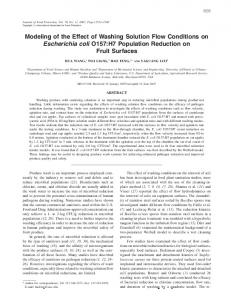
They concluded that using two baffles in suitable position achieve reducing the size of the circulation zone, kinetic energy in sedimentation area, maximum velocity magnitude and create uniform velocity vector inside the settling zone. In present work, the investigations on the baffle position effects on the settling efficiency are performed via some experiments and computational simulation using Flow-3D [12]. It must be noted that the use of baffles without enough concern would result in tanks with the worse performance than the tank without a baffle. A baffle’s cost is also high. These make it essential to investigate the best position of the baffles in settling tanks. In experimental part of the work, the mixture of water and suspended sediments were made to enter the settling tank and a thin baffle is positioned in a laboratory settling tank and the effects of its position on the velocity of flow field (with using Acoustic Doppler Velocimeter) and sediment concentration in the tank were measured. Then, numerical experiments are performed for baffle installation in different distances from the inlet of the tank via sediment scour model. In this study to find the best location of baffle, velocity profile, volume of circulation zone, kinetic energy, suspended sediment concentration and removal efficiency was investigated for different location of baffle installation. The results of the numerical simulation and experimental tests show that primary sedimentation tank performance can be improved by altering the geometry of the tank. The effects of baffle positions on the efficiency of the primary sedimentation tank were investigated by assessing the magnitude of the concentration of the suspended sediments, the circulation zone volume variations, the velocity values and finally, the removal efficiency in the flow field of each case. Laboratory Model Laboratory Setup Details: A set of laboratory measurements was conducted in a rectangular primary sedimentation tank with water depth to tank length ratio of 0.155. Figure 1 illustrates the experimental setup and measurement system. This figure shows a rectangular primary settling tank with a length (L) of 200 cm, width (W) of 50 cm, height (H) of 31 cm, inlet opening height (Hin) of 10 cm, weir height (H )w of 30 cm. An electromagnetic flow meter was used to measure the volumetric flow of conductive liquid. This flow meter is composed of a sensor and an electromagnetic flow rate transducer. Particles precipitated from previous runs were removed and conducted out of the channel.
1297
World Appl. Sci. J., 15 (9): 1296-1309, 2011
Fig. 1(a): schematic diagram of the tank; (b) A photo of baffle in the tank; (c) A Photo of laboratory setup Each experimental result did not exhibit the same degree of influence as that observed in the re-suspension from previous runs. The laboratory experiments were conducted for the settling tank without baffle with flow rate equal to Q=2 L/s. the value of inlet Reynolds number equal to Rein =3972. The Froude Number in the inlet and in the tank were Frin=0.04 and Fr=0.0075, respectively. Laboratory Measurement Device: The three velocity components are measured using Acoustic Doppler Velocimetry (ADV). A 10 MHz Nortek acoustic Doppler velocity meter is used for measuring instantaneous velocities of the liquid flow at different points in the tank. Measurements are performed by measuring the velocity of particles in a remote sampling volume based upon the Doppler shift effect [13, 14]. The probe head includes one transmitter and four receivers. The remote sampling volume is located 5 or 10 cm from the tip of transmitter, but some researchers showed that the distance might change slightly [15], so this is the advantage of the ADV, while the probe is inserted into the flow, the sensing volume is away from the probe and the presence of the probe generally does not effect on the measurement. The accuracy of the measured data is no greater than ±0.5% of measured value ± 1 mm/s, sampling rate output is between 1-25 Hz, random noise approximately equal to 1% of the velocity range at 25 Hz [16]. There are some assumptions when applying ADV in a turbidity flow. First the velocity measured by ADV is related to the velocity of fine particles suspended in the fluid. ADV measures the change in frequency of the
returned sound from fine particles suspended in the water. These fine particles are assumed to move at the same velocity as that of the fluid. Thus, to use ADV, very fine particles of zeolite with low concentrations are added as a seeding material to the water. The second assumption is that the changes in density or density layer of the fluid cause changes in the acoustic velocity. Whereas the sediment concentration in the dense fluid was measured up to 15 g/l, this value was actually lower during the experiments. Therefore, there were no significant changes in the acoustic velocity [17]. After measuring the instantaneous velocity with ADV, the post-processing process should be done on collected data before calculating the flow characteristics. In steady flows, the first step of signal processing is the elimination of all data samples with communication errors, average correlation below 70% or signal-to-noise ratio (SNR) below 15 dB. Then the data may be "despiked" using the phase-space thresholding technique (using WinADV 2.025). In this research ADV is located enough far from the solid boundaries, so the solid boundaries do not effect on the measuring data. Laboratory Concentration Measurement: In this section, the fine sediment was interred into the tank and its concentration from inlet to outlet in at different points was measured to obtain the vertical distribution of concentration. With the system not circulated, the water with suspended sediment concentration (SSC) drained from the flume and flowed to the basin was taken either from an indoor reservoir via tap water. Consequently, tap water was not circulated back to the indoor reservoir,
1298
World Appl. Sci. J., 15 (9): 1296-1309, 2011
resulting in the tank entry getting filled with clear tap water. A pipe was attached at the center of the inlet slot of the sedimentation basin. The diameter of the sediment slurry inflow opening was 0.4 cm. Figure 2 shows the inlet aperture and the pipe that transfer sediment slurry into the tank. The pipe was a silicone tubing directly connected to the mixing box of sediment slurry via one Masterflex pump. The height and width of the inlet slot opening were 10 cm and 50 cm, respectively. The pipe transfers the sediment slurry at a constant discharge of 30 ml/min. The discharge of water through the inlet slot was equal to 2 l/s. When combined, the velocity of the tap water in the inlet slot and the velocity of the sediment slurry in the pipe was the same. Consequently, the proper mix of sediment slurry and water were created in the inlet of the sedimentation tank. Zeolite was used as the suspended sediment for the physical model because its particles do not possess high cohesive properties and have low density, approximately equal to that of water. The density of such particle is 1.049 g/cm3, which is very close to the density of water. Particle size distribution was classified into two classes. Half of the sediment particles have diameters between 75 and 106 µm; the diameters of the other half are between 106 and 150 µm. The particle concentrate was prepared in a 20 L bucket mixed by the circulation created by a submersible pump at the bottom of the mixing bucket. The submersible pump draws sediment slurry from the bottom of the bucket and pushes it out through the 1.25 in diameter opening at the rate of 2.2 L/s. The opening angle was set al. most parallel to the bottom to enhance scouring and re-suspension of zeolite particles. Mixed particle concentrate was delivered using a Masterflex pump (L/S® variable-speed economy drive, Model No: 7524-45), the flow rate of which can be kept constant. The flow rate of the pump was controlled digitally and with the correct tubing size and flow rate, the pump was ready to transfer the sediment slurry into the settling tank. Masterflex platinum-cured silicone tubing (Model No: 96400-16) was used to transfer the sediment slurry into the tank. The flow rate of this model of tubing can adjust between 4.8 and 480 ml/min. Masterflex large cartridges (Model No: 07519-05) were chosen for this tubing model. During the experiment, the flow rate of interring the sediment slurry into the tank was set to 30 ml/min.
Fig. 2: Inlet aperture and the pipe that transfer sediment slurry into the tank
Fig. 3: Masterflex pump and the bottle used for taking the sample Suspended Sediment Concentration Measurement: The length and height of the settling tank were divided into six points to measure the concentration of SSC. The samples were taken at a height of 5 cm and a length of 37 cm in each tank using Masterflex pumps. These pumps are very useful for taking samples because it is possible to adjust the speed of sampling digitally. In these experiments, Masterflex L/S® variable-speed economy drive (Model no: 7524-45, 10-600 rpm, 230V) was used. The flow rate of this pump is adjustable between 0.6 and 3400 ml/min. Masterflex platinum-cured silicone tubing (Model No: 96410-14) was used to take samples inside the settling tank and to decrease the effect of the large size of tubing on the flow field of the settling tank. The inside diameter of this tubing measured 1.6 mm and the flow rate range was 1.3–130 ml/min. The speed of taking samples is very important because if it is greater than the velocity of the real fluid in the settling tank, it can disrupt the flow in the tank. During the experiment, the flow rate for taking samples was set to 2 ml/min; thus, with this flow rate, the speed of taking the sample was equal to the average velocity of the flow in the settling tank. Masterflex small cartridges (Model No: 07519-80) were chosen for this tubing model. At the beginning of the experiment, the sediment was interred to the tank for 4 min to make the sediment flow distribution uniform. After that for 15 min, the samples were then taken from inside the tank. Figure 3 represents the Masterflex pump and the bottle used for taking the sample from inside the settling tank.
1299
World Appl. Sci. J., 15 (9): 1296-1309, 2011
For measuring the concentration of the suspended sediment in each sample, a turbidimeter (HANNA Instrument HI 98703) was used. The instrument is specially designed for water quality measurements, providing a reliable and accurate reading on low turbidity values. The instrument is used to measure the turbidity of a sample in the 0.00 to 1000 Nephelometric Turbidity Units (NTU) range. Conversion of this unit (NTU) to the other units is possible. The instrument is based on an optical system, which guarantees accurate results. The optical system, consisting of a tungsten filament lamp and two detectors (scattered and transmitted), assures long-term stability and minimizes stray light and color interferences. The microprocessor of the instrument calculates from the signals that reach the two detectors (the NTU value) using an effective algorithm. It also compensates for variations in the intensity of the lamp, minimizing the need for frequent calibration. Turbidity of the water is an optical property that causes light to be scattered and absorbed, rather than transmitted. The scattering of the light that passes through liquid is primarily caused by suspended solids. The higher the turbidity, the greater is the amount of scattered light. Given that even the molecules in a very pure fluid scatter light to a certain degree, no solution has zero turbidity. Compuational Model Mathematical Model Time-Averaged Flow Equations: Steady state incompressible flow conditions with viscous effect are generally considered in hydraulic numerical modeling and the Navier–Stokes equation has been well-verified as an effective solution to the governing equation. The Navier–Stokes equation is an incompressible form of the conservation of mass and momentum equations and is comprised of non-linear advection, rate of change, diffusion and source term in the partial differential equation. The mass and momentum equations joined by velocity can be used to obtain an equation for the pressure term. When the flow field is turbulent, computation becomes more complex. Because of this, the Reynolds-Averaged Navier–Stokes (RANS) equation is prevalently used. It is a modified form of the Navier–Stokes equation and includes the Reynolds stress term, which approximates the random turbulent fluctuations by statistics. The governing equations are general mass continuity and momentum. The turbulence model is also solved with these equations to calculate the Reynolds stresses.
The mass continuity equation for fluids is simple. The flow pattern is assumed to be two-dimensional, enabling the calculation of two momentum equations in the x and z directions, as well as the length and height of the tank. The general mass continuity equation is [18, 19]. Vf
∂ ∂ ∂ + ( uA) + ( wAz ) = 0 ∂t ∂x ∂z
(1)
Where Vf is the fractional volume of flow in the calculation cell; is the fluid density; and (u,w) are the velocity components in the length and height (x, z). The momentum equation for the fluid velocity components in the two directions are the Navier–Stokes equations, expressed as follows: ∂u 1 ∂u ∂u 1 ∂P + + wAz = − + Gx + f x uAx ∂t V f ∂t ∂z ∂x ∂w 1 + ∂t V f
(2)
∂w ∂w 1 ∂P + wAz + Gz + f z uAx =− (3) ∂ ∂ ∂z x z
Where Gx, Gz are body accelerations and fx, fz are viscous accelerations. Variable dynamic viscosity µ are as follows: ∂ Vf fx = wsx − ( Ax ∂x
xx
)+
∂ ( Az ∂z
xz
)
(4)
∂ Vf fz = wsz − ( Ax ∂x
xz
)+
∂ ( Az ∂z
zz
)
(5)
Where
∂u ∂w ∂u ∂w −2µ , t zz = −2µ −µ + t xx = , t xz = ∂x ∂z ∂z ∂x (6)
Where, the parameters wsx and wsz are wall shear stresses, respectively. The wall stresses are modeled by assuming a zero tangential velocity on the boundary points for turbulent flows and a law-of-the-wall velocity profile is imposed near the wall boundaries of the domain, which modifies the wall shear stress magnitude [13]. Fluid surface shape is illustrated by volume of fluid (VOF) function F(x, z, t). With the VOF method, grid cells are classified as empty, full, or partially filled with fluid. Cells are allocated in the fluid fraction varying from zero to one, depending on fluid quantity. Thus, in F=1, fluid exists, whereas F=0 corresponds to a void region. This function displays the VOF per unit volume and satisfies the equation [18].
1300
World Appl. Sci. J., 15 (9): 1296-1309, 2011
(9) Where P represents the shear production, G is the buoyancy production, Diff and Ddif represent diffusion and C1 , C2 , C3 are constants. In the RNG model, C1 = 1.42, C2 = 1.68 and C3 = 0.2 [20, 21]. In particular, the RNG model is known to describe lowintensity turbulence flows and flows having strong shear regions more accurately.
increase the solution consistency and the results are more accurate. These semi-implicit formulations of the finite-difference equations enable the efficient resolution of low speed and incompressible flow problems. The semi-implicit formulation, however, results in coupled sets of equations that must be solved by an iterative technique [12]. The computational fluid dynamics (CFD) program in FLOW-3D® solves the RANS equations by the finite volume formulation gained from a rectangular finite difference grid. For each cell, mean values of the flow parameters, such as pressure and velocity, are calculated at discrete times. The new velocity in each cell is computed from the coupled momentum and continuity equation using previous time step values in each of the centers of the cell faces. The pressure term is obtained and adjusted using the estimated velocity to satisfy the continuity equation. With the computed velocity and pressure for a later period, the remaining variables are estimated involving turbulent transport, density advection and diffusion and wall function evaluation [12]. In the utilized software, the boundary condition for the inflow (influent) is considered as constant velocity and free outflow condition was selected for the outlet (effluent). No slip conditions were applied at the non-penetrative rigid walls and the law-of-the-wall velocity profile was imposed near the wall surface, which modifies the wall shear stress magnitude. The position of free surface boundary was calculated by application of the VOF method [18]. In addition, the Fractional Area/Volume Obstacle Representation (FAVOR) method can be used to inspect the geometry in the finite volume mesh [19]. FAVOR appoints the obstacles in a calculation cell with a factional value between zero to one as obstacle fills in the cell. The geometry of the obstacle is placed in the mesh by setting the area fractions on the cell faces along with the volume fraction open to flow [22]. This approach creates an independent geometry structure on the grid and then the complex obstacle can be produced.
Numerical Solver: In this paper, a module of FLOW-3D® flow solver (version 9.4.1), which utilizes a finite volume is used to simulate the free surface flow in these tanks. The flow field is separated into fixed rectangular cells. The local average values of all dependent variables for each cell are computed. Pressures and velocities are associated implicitly by using time-advanced pressures in momentum equations and time-advanced velocities in the mass (continuity) equation. The implicit schemes will
Sediment Scour Model: In FLOW-3D the sediment scour model (estimates the motion of sediment flow by predicting the erosion, advection and deposition of sediment) is done by considering two types in which sediment can exist as suspended and packed sediment. Suspended sediment is typically of low concentration and advects with fluid. Packed sediment does not move with any fluid and exists in the computational domain at the critical packing fraction.
1 ∂ ∂F ∂ + 0 ( FAx u ) + ( FAz w) = (7) ∂t V F ∂x ∂z
F in one phase problem depicts the volume fraction filled by the fluid. Voids are regions without fluid mass that have a uniform pressure appointed to them. Physically, they represent regions filled with vapor or gas, whose density is insignificant in relation to fluid density. Turbulent model: To model turbulence, the RNG model was used and turbulent viscosity was computed using a differential equation. The RNG model is practical for cases with curved streamlines, as in circulation regions and applies statistical methods to derive the averaged equations for turbulence quantities, such as turbulent kinetic energy and its dissipation rate. RNG-based models rely little on empirical constants while setting a framework for the derivation of a range of models at different scales [20, 21]. The RNG model uses equations that are similar to those for the k– model. However, the equation constants found empirically in the standard k– model are derived explicitly in the RNG model. The turbulence kinetic energy, k and its rate of dissipation, , are obtained from the following transport equations: ∂k 1 ∂k ∂k + + wAz uAx = P + G + Diff − ∂t VF ∂x ∂z ∂ ∂t
+
1 VF
{
uAx
∂ ∂x
+ wAz
∂ ∂z
}
=
C1 . k
( P + C3
.G ) + DDif − C2 .
(8) 2
k
1301
World Appl. Sci. J., 15 (9): 1296-1309, 2011
Suspended sediment is transported by advection along with the fluid. Therefore, without considering the VOF and FAVOR functions, the transport equation is:
( )
∂C s
+ ∇. uC s = 0
∂t
(10)
Where Cs is the concentration of the suspended sediment, in units of mass per unit volume and u is the mean velocity of the fluid/sediment mixture. Because sediments typically have a density greater than the surrounding flow, they will sink, or drift, relative to the surrounding flow. The drift velocity is computed based on the assumption that the drift sediment particles can be considered. This is true so long as the particles do not interact with one another, which is usually true for particles in suspension. The rate of this drift is related to the balance between the buoyancy force and the drag force. Therefore, one can write momentum balances for each sediment species and the fluid-sediment mixture (again neglecting the VOF and FAVOR functions): ∂u s ∂t ∂u ∂t
+ u.∇u s =−
+ u.∇ u = −
1
1
fs
ur =
s
ur
∇P Ki
(
s
Where the mixture density,
∑f
1 − u= fs u f +
(13)
= K
g Ki
(
s
−
1
+ u.∇udrift=
)f
s
3 fs
C D ur + 24 4 d s
u drift = (1 − f s ) ur −
∑
f su s
(17)
(18)
−
1 s
Ki
∇P − fs
s
ur
(15)
f ds f
(19)
N ( −i )
∑ j =1
(14)
Where N is the total number of sediment species. Subtracting Eq. (12) from (11) gives
∂t
f
Where ds and CD are the diameter and the drag coefficient for sediment, respectively and µf is the fluid viscosity. Finally, the drift velocity is computed from the relative velocity using the definition of the drift and relative velocities:
N
= j 1= j 1
∂udrift
Note that in many simulations the pressure gradient can become very noisy, mostly close to the free surface. For most problems the ratio of pressure gradient to mixture density is typically equal to the acceleration of gravity, g. With this assumption we get:
and the mean velocity is
s
(12)
ur = us – u f
∑
(16)
A reasonable choice for the drag function K combines form drag and Stokes drag:
∇P + F
N
s
N
∑f
1− s s + i 1 =i 1 =
(11)
Here us is the velocity of sediment particles, iss the density of the sediment material, fs is the volume fraction of sediment, P is the pressure, K is the drag function, F includes body and viscous forces, ui is the relative velocity,
)f
−
, is
N
=
ur =
K
∇P + F −
Where udrift= u s − u is the drift velocity, i.e., the velocity needed to compute the transport of sediment due to drift. Assuming that the motion of the sediment is nearly steady at the scale of the computational time and that the advection term is small (i.e., for small drift velocity udrift), the result of Equation (15) is:
f sur
(20)
Equations (16), (17) and (18) are solved via the quadratic formula to find udrift. Sediment is entrained by the picking up and resuspension of packed sediment due to shearing and small eddies at the packed sediment interface. Because it is not possible to compute the flow dynamics about each individual grain of sediment and it is oftentimes difficult 1302
World Appl. Sci. J., 15 (9): 1296-1309, 2011
to compute the boundary layer at the interface, an empirical model must be used. The model used here is based on [23]. Also, the Shields-Rouse equation [24] can be used to predict the critical Shields number, or a user-defined parameter can be specified. The first step to computing the critical Shields number is calculating the dimensionless parameter R* : 0.1
*
R = ds
(
s
−
f
)
g ds
f
(21)
f
and from this, the dimensionless critical Shields parameter is computed using the Shields-Rouse equation [24]: −R 0.1 = + 0.054 1 − exp 2 10 * R 3
*0.52
cr
(22)
Also included in the model are the effects of armoring, whereby larger sediment particles protect finer particles from becoming entrained. The critical Shields parameter is then modified by the effects of armoring [25]: '
cr
=
1.666667
cr
ds
d 50
log10 19
(23)
2
Note that, according to Eq. (24), if ds is far smaller than d50, the denominator will be a small number and thus enhance the value of 'cr ,i , because the finer particles are surrounded by larger particles. Conversely, for values of di much larger than d 50, Eq. (23) will serve to reduce it, because the coarser particles are more exposed when surrounded by finer particles. The local Shields number is computed based on the local shear stress, : =
g ds
(
s
−
f
)
(24)
Where d* is the dimensionless mean particle diameter, d* = d50
ulift =
ns d*
0.3
(
−
cr
)1.5
(
s f
−
f
)
(25)
(
s
−
f
)g
2
1
3
(26)
is the entrainment parameter, whose recommended value is 0.018 [23] and ns is the outward pointing normal to the packed bed interface. ulift is then used to compute the amount of packed sediment that is converted into suspended sediment, effectively acting as a mass source of suspended sediment at the packed bed interface. Once converted to suspended sediment, the sediment subsequently advects and drifts [12]. The most important parameters for simulating sedimentation process are sediment density, diameter and critical Shields number. The numerical simulation were done for six cases with the same flow rate (equal to Q=2 L/s). Case 1 had no baffle; in cases 2 to 6, a baffle was placed in various distances: inlet-to-tank length ratios of (d/L)=0.10, 0.125, 0.20, 0.30 and 0.40 (using a baffle height-to-depth ratio of Hb/H=0.18). Verification Test: In order to verify the results of computational model, the experimental conditions of the settling tank which mentioned before for the case without baffle was considered. To find the accuracy of the empirical results, the data was plotted on a graph and a fit curves to quantify the scatter of data and determine whether any special trend exists. A polynomial in order n is fitted to data points to find the velocity profile in each section. Figures 4 (a), (b) illustrates a typical experimental data and standard deviations at x/L=0.41 for a tank without baffle. The following relation is then used as the best estimate for standard deviation [26]. 1 = n − 1
∑ ( ui − u )
1/ 2 2
(27)
In which ui is the measured velocity and û is the average velocity in x direction as follows:
Here ||g|| is the magnitude of the gravitational vector. The entrainment lift velocity (volumetric flux) of sediment is then computed as [23]: g ds
f
u=
1 n
n
∑ ui i =1
(28)
The obtained data are shown in Figure 4(b). Higher values of standard deviations mean more uncertainty in the results. The systematic and random 1303
World Appl. Sci. J., 15 (9): 1296-1309, 2011
Fig. 4(a): The curve is fitted to the velocity measured data at x/L=0.41; (b) The standard deviation of the results
Fig. 5(a): Comparison of x-velocity component for the case without baffle; (b) Comparison of vertical distribution of SSC for the case without baffle at (a)47 cm, b)84 cm, (c)121 cm, (d)158 cm, (e)195 cm errors being associated with the measurement in experiment or instrumentation, or both, must be analyzed for a perfect correction. It should be mentioned that in this experiment the temperature fluctuation is one of the important source of errors. The measured values of dimensionless x- velocity and vertical distribution concentration of the suspended sediments are shown in Figures 5 (a) and (b), respectively. In this study, the numerical model was applied to simulate this basin using a uniform rectangular mesh. The boundary condition for the influent is the constant velocity, whereas those selected for the outlet (effluent) is the outflow condition. No slip conditions were applied at the rigid boundaries and these were treated
as non-penetrative boundaries. With no-slip boundary, it is assumed that a law-of-the-wall type profile exists in the boundary region, which modifies the wall shear stress magnitude. In addition, the symmetry condition is applied for zero gradient perpendicular to the boundary. The influent flow rate and sediment concentration is 2 l/s and 100 mg/l, respectively. The flow in the sedimentation tanks is in reality three-dimensional, especially in the inlet section of the tank. This is related to the position of the inlet and outlet of tank, as well as their opening sizes. For simplicity, the flow field can be represented as two-dimensional vertical plane models because in the current study, the inlet and outlet spread out all over the width of the tank.
1304
World Appl. Sci. J., 15 (9): 1296-1309, 2011
Some numerical simulations were thus conducted with various numbers of cells to find the grid-independent solution. Finally, a 69× 288 grid with approximately 19872 cells was chosen for the computation modeling. The numerical results show good agreement with experimental data, but some errors for velocity values are observed near the bed, particularly in the regions near the inlet zone. The discrepancies between the result of the computational model and experimental measurements are probably due to the differences of the flow patterns in the inlet section. Although there is a uniform velocity profile in the numerical model, this condition differs from experimental tests. Also the discrepancy in the SSC measurements between the experimental and numerical simulation results are related to the assumption the flow two-dimensional. So in experimental test some of the sediments particles distribute to width direction of the tank, consequently the numerical model can be predicted the results of the SSC more than the values of experimental tests. However, the SSC results of the numerical model have good trend and accuracy in comparison with the experimental results. RESULTS AND DISCUSSION Discussion on Velocity Laboratory Measurements: To increase the efficiency of the sedimentation tank, the numerical simulation of the above mentioned cases were conducted. The best location for the baffle is obtained when the volume of the circulation zone is minimized or the recirculation region forms a small portion of the flow field. Circulation volume, which is normalized by the total water volume in the tank and calculated by the numerical
Fig. 6:
Volume of the circulation zone according to amount of distances from the inlet to tank length ratios (d/L)
method, is shown in Figure 6. The table indicates the absolute predictability of some cases to exhibit weak performance because of the size of the dead zone. Figure 6 shows that the baffle position at d/L=0.125 has minimum magnitude of circulation volume and consequently exhibits the best performance. In addition, this Figure indicate that if baffle is located in worse position, the efficiency of this tank maybe less than a tank without any baffle. Consequently, it is necessary to investigate about the best position and configuration of the baffle in settling tank. The streamline of different baffle locations in the sedimentation tank are shown in Figure 7. Two circulation zones exist in the tank at d/L=0.125. The circulation volume, however, remains minimized and the baffle presumably separates the dead zone into two sections. The comparison between cases that baffle at d/L=0.125
Fig. 7: Computed streamlines for a)d/L=0.10, b)d/L=0.125, c)d/L=0.20, d)d/L=0.30, e)d/L=0.40 and f)No baffle 1305
World Appl. Sci. J., 15 (9): 1296-1309, 2011
Fig. 8: Computed kinetic energy for a) no baffle, b) d/L=0.125
Fig. 9: Computational results, comparing no baffle and baffle at d/L=0.125 for a baffle height (Hb/Hw =0.18) and no baffle in Figure 8 shows that using the baffle in the settling basin causes the kinetic energy decrease near the bed and the zone with high kinetic energy moves to the upper region of the basin. The baffle creates a region with low amounts of kinetic energy near the bed. The ability of flow to carry the sediment is not significant and the sedimentation process may increase. Figure 9 illustrates the result of the numerical simulations, in which parameters such as velocities in x and z directions (i. e. u and w respectively), as well as kinetic energy in the tank with (at d/L=0.125 for the baffle case with height to depth ratio Hb/Hw=0.18) and without baffle, were compared. The using baffle in the proper position can reducing the velocities in x and z directions in the settling zone of the tank (after baffle position) and make good opportunity for trapping the particles because of the existence uniform and calm velocity field. The presence of a baffle causes increasing turbulent kinetic energy before baffle location, but after, a significant decrease in the quantity of the turbulence kinetic energy is observed. So this means that the
tendency to create a uniform flow in the tank which baffle is located at d/L=0.125 is greater compared to the tank without a baffle. In addition, the slop of velocity profile near the bed is low which means that after the baffle, the shear stress decreases on the bed. The behavior of the flow tends to be calm at the remaining part of the tank so that the baffle can mix current in the flow field right after passing it. Concentration Laboratory Measurements: The theory was used in this part of the simulation is that if a sedimentation tank keeps more sediment particles inside the settling zone; it would attain higher removal efficiency. This trend means that more suspended sediments have the opportunity to be deposited in the settling area at the same time. The SSC inside the settling tank was higher than the other baffle installation positions where the baffle was located from d/L=0.125 to d/L=0.20; the highest SSC was achieved when the baffle was located at d/L=0.125 (Figure 10). 1306
World Appl. Sci. J., 15 (9): 1296-1309, 2011
Fig. 10: Vertical distribution of the suspended sediments concentration along the length of the settling tank at (a)47 cm, b)84 cm, (c)121 cm, (d)158 cm, (e)195 cm = R (%)
Fig. 11: Sediment removal efficiency for various baffle distances from the inlet to tank length ratios (d/L) The measured data of SSC for different cases of experiments prove the outcome of circulation zone volume analysis. The location of the baffle at d/L=0.125 created the lowest value of circulation volume and the maximum amount of SSC in the settling tank. A baffle located between d/L=0.125 and d/L=0.20 seems to suppress the horizontal velocities and kinetic energy effectively, putting force on the suspended sediments to move to the bottom of the tank, thereby reducing the chance for short-circuit to occur. Removal Efficiency Measurements: In this part the solution of the water and sediment was interred to the tank for 15 min. Subsequently, the discharge of sediment was stopped. Then for the duration equal to detention time, clear water flow into the tank. After that the mass of sediment which were interred and settled on the bottom of the tank were measured. Finally the removal efficiency of the settling tank can be achieved by
M settled sediment M interredsediment
× 100
The results of measurements of suspended sediment removal efficiency are shown in Figure 11. An optimum value of the relative location of the reaction baffle existed, under which the highest removal efficiency could be achieved. As the baffle distance from d/L was increased from 0.125 to 0.40, the removal rate decreased from 22.53% to 15.48%. With increasing distance of the baffle location from the inlet slot, the return of the circulation flow increased and the jet effect intensified at the bottom of the baffle. As the baffle distance from d/L was reduced from 0.125 to 0.10, its removal efficiency dropped from 22.53% to 17.38%. Therefore, the smaller the baffle distance, the weaker is its energy dissipation effect. As a result of the experimental test related to the velocity measurement of the flow field, SSC measurement and calculation removal efficiency, an optimum location for the baffle between d/L=0.125 to d/L=0.20 is recommended. CONCLUSION Sedimentation by gravity is one of the most common and extensively applied techniques in the removal of suspended solids from water and wastewater. Investment in settling tanks accounts for about 30% of the total investment in a treatment plant. The calculation of sedimentation performance has been the subject of numerous theoretical and experimental studies. Sedimentation performance depends on the characteristics of the suspended solids and flow field in the tank. A uniform and calm flow field is essential for a tank to have high efficiency. This facilitates particle
1307
World Appl. Sci. J., 15 (9): 1296-1309, 2011
deposition at a constant velocity in less time. In general, circulation regions are always present in settling tanks. Circulation zones are named dead zones, because water is trapped and particulate fluid will have less volume for flow and sedimentation in these regions. The existence of large circulation regions, therefore, lowers tank efficiency. Moreover, the formation of circulation zones diminishes the performance of the sedimentation tank by short circuiting and positioning a baffle in an appropriate location can reduce the formation of these zones. This means that correctly positioning a baffle prevents the formation of the bottom jet moving to the surface of the basin and spilling over at the outlet. In this study, numerical simulation was performed to investigate the effects of baffle location on the flow field. The results of this computational model prove that the baffle should be placed between 0.125 and 0.20 (d/L) based on the smallest volume of the circulation zone and kinetic energy, the maximum concentration of the suspended sediments in the settling zone and the highest value of removal efficiency. REFRENCES 1.
2. 3. 4.
5.
6.
7.
8.
9.
10.
11.
12. 13.
14.
Krebs, P., D. Vischer and W. Gujer, 1995. Inlet-structure design for final clarifiers. J. Environmental Engineering, ASCE, 121(8): 558-564. Metcalf, Eddy, 2003. Wastewater engineering treatment and reuse. McGraw-Hill, New York. Kawamura, S., 2000. Water Treatment Facilites. John Wiley and Sons, Inc. Tamayol, A., B. Firoozabadi and G. Ahmadi, 2008. Effects of Inlet Position and Baffle Configuration on Hydraulic Performance of Primary Settling Tanks. J. Hydraulic Engineering, ASCE., 134(7): 1004-1009. Zhou, S., J. McCorquodale and Z. Vitasovic, 1992. Influences of density on circular clarifiers with baffles. J. Environmental Engineering, ASCE, 118(6): 829-847. Bretscher, U., P. Krebs and W.H. Hager, 1992. Improvement of flow in final settling tanks. J. Enviromental Engineering, ASCE, 118(3): 307-321. Goula, A.M., M. Kostoglou, T.D. Karapantsios and A.I. Zouboulis, 2007. A CFD methodology for the design of sedimentation tanks in potable water treatment case study: the influence of a feed flow control baffle. Chem. Eng. J., 140: 110-121.
15.
16. 17.
18.
19.
20.
1308
Huggins, D.L., R.H. Piedrahita and T. Rumsey, 2005. Analysis of sediment transport modeling using computational fluid dynamics (CFD) for aquaculture raceways. Aquacult. Eng., 31: 277-293. Razmi, A.M., B. Firoozabadi and G. Ahmadi, 2008. Experimental and Numerical Approach to Enlargement of Performance of Primary Settling Tanks. J. Applied Fluid Mechanics, 2(1): 1-13. Liu, B., J. Ma, L. Luo, Y. Bai, S. Wang and J. Zhang, 2010. Two-Dimensional LDV Measurement, Modeling and Optimal Design of Rectangular Primary Settling Tanks. J. Environmental Engineering, ASCE, 136(5): 501-507. Shahrokhi, M., F. Rostami and M.A.M. Said Syafalni, 2011. The Computational Modeling of Baffle Configuration in the Primary Sedimentation Tanks. 2th ICEST, pp: 392-396. FlowScience, 2009. Flow-3D user manual. in. Voulgaris, G. and J.H. Trowbridge, 1998. Evaluation of the Acoustic Doppler Velocimeter (ADV) for Turbulence Measurements J. Atmospheric and Oceanic Technologies, 15: 272-289. McLELLAND, S.J. and A.P. Nicholas, 2000. A New Method for Evaluating Errors in High-Frequency ADV Measurements. Hydrological Processes, 14: 351-366. Chanson, H., S. Aoki and M. Maruyama, 2000. Unsteady Two-Dimensional Orifice Flow: an Experimental Study. in, Toyohashi University of Technology, Japan. Nortek, 2004. Nortek Vectorino Velocimeter-User Guide. in. Kawanisi, K. and S. Yokosi, 1997. Measurements of suspended sediment and turbulence in tidal boundary layer. Continental Shelf Research, 17: 859-875. Hirt, C.W. and B.D. Nichols, 1981. Volume of Fluid (VOF) Method for the Dynamics of Free Boundaries. J. Comp. Phys., 39: 201-225. Hirt, C.W. and J.M. Sicilian, 1985. A Porosity Technique for the Definition of Obstacles in Rectangular Cell Meshes. in: Fourth International Conf. Ship Hydro., National Academy of Science, Washington, DC, pp: 1-19. Yakhot, V. and S.A. Orszag, 1986. Renormalization Group Analysis of Turbulence. I. Basic Theory. J. Scientific Computing, 1: 1-51.
World Appl. Sci. J., 15 (9): 1296-1309, 2011
21. Yakhot, V. and L.M. Smith, 1992. The Renormalization Group, the e-Expansion and Derivation of Turbulence Models. J. Scientific Computing, 7: 35-61. 22. Hirt, C.W., 1992. Identification and Treatment of Stiff Bubble Problems. in, Flow Science Inc. 23. Mastbergen, D.R. and J.H. VondenBerg, 2003. Breaching in fine sands and the generation of sustained turbidity currents in submarine canyons. Sedimentology, 50: 625-637.
24. Guo, J., 2002. Hunter Rouse and Shields diagram. Proc 1th IAHR-APD Congress, pp: 1069-1098. 25. Kleinhaus, M.G., 2002. Sort out sand & gravel: sediment transport and deposition in sand-gravel bed rivers. in, Universitaat Utrecht. 26. Nikora, V.I., D.G. Goring and A. Ross, 2002. The structure and dynamics of the thin near-bed layer in a complex marine environment. Estuarine, Coastal and Shelf Sci., 54: 915-926.
1309