Numerical Modeling of the Seismic Performance of Bituminous Faced ...

M. Albano Numerical modeling of the seismic performance of bitumionous faced rockfill dams

Among the various possible types, the embankment dams with bituminous concrete facing represent an important category, being largely present in the Italian territory and worldwide. From a structural viewpoint, these manufacts are particularly challenging, not only due to their uncommon dimensions and the very high risk potentially connected with their malfunctioning, but also because their mechanical and hydraulic behaviour is dictated by a complex of interlocked factors, not always easy to investigate, characterize and predict. By no means the coupling between embankment, foundation and non-structural components, can be overlooked when performing analyses. The tight coexistence of the granular materials forming the embankment with the multi-composed waterproofing system is a factor of great complexity. Additionally, while support and watertightness functions should be kept clearly distinguished, their interactions are often unavoidable. Geometrical irregularity of the basement and heterogeneity of materials are other factors increasing the complexity of the problem. The role of all these aspects, fundamental when gravity loads induced by normal operating condition are the only applied actions, is even more emphasized when the dam is subjected to extraordinary loading conditions such as those determined by earthquake events. The design of these structures, like the design of any other structure, has to be developed through a number of logical steps, going from characterization of materials to cost assessment, and passing through the considerations on limit states and the respect of standards and Codes of Practice as typical in civil engineering. Investigation and calculation tools allow to get increasingly larger confidence in such kind of analyses. What is new, and strictly related to the problem dealt with in this thesis, is the relevance of the aforementioned aspects in the assessment of existing structures, often designed and controlled with out of date procedures and for which information are often incomplete or totally lacking. The challenge of this research is to investigate by means of numerical modeling, the aspects governing the seismic response of rockfill dams with bituminous concrete face, with the aim of defining a comprehensive assessment procedure for both new and existing manufacts, eventually leading to a rational design of rehabilitation.

Matteo Albano

Numerical Modeling of the Seismic Performance of Bituminous Faced Rockfill Dams Doctoral thesis

University of Cassino and Southern Lazio Department of Civil and Mechanical Engineering

UNIVERSITÀ DEGLI STUDI DI CASSINO E DEL LAZIO MERIDIONALE SCUOLA DI DOTTORATO IN INGEGNERIA DIPARTIMENTO DI INGEGNERIA CIVILE E MECCANICA

Numerical modeling of the seismic performance of bituminous faced rockfill dams Matteo Albano

In Partial Fulfillment of the Requirements for the Degree of PHILISOPHIAE DOCTOR in Civil Engineering XXV Cycle

TUTOR Prof. Paolo Croce

COORDINATOR Prof. Giuseppe Modoni

UNIVERSITÀ DEGLI STUDI DI CASSINO E DEL LAZIO MERIDIONALE SCUOLA DI DOTTORATO IN INGEGNERIA

Date: January 2013 Author:

Matteo Albano

Title:

Numerical modeling of the seismic performance of bituminous faced rockfill dams

Department: Department of Civil and Mechanical Engineering Degree:

Philosophiae Doctor

Permission is herewith granted to University to circulate and to have copied for noncommercial purposes, at its discretion, the above title upon the request of individuals or institutions.

_____________________________ Signature of Author

THE AUTHOR RESERVES OTHER PUBLICATION RIGHTS, AND NEITHER THE THESIS NOR EXTENSIVE EXTRACTS FROM IT MAY BE PRINTED OR OTHERWISE REPRODUCED WITHOUT THE AUTHOR’S WRITTEN PERMISSION. THE AUTHOR ATTESTS THAT PERMISSION HAS BEEN OBTAINED FOR THE USE OF ANY COPYRIGHTED MATERIAL APPEARING IN THIS THESIS (OTHER THAN BRIEF EXCERPTS REQUIRING ONLY PROPER ACKNOWLEDGEMENT IN SCHOLARLY WRITING) AND THAT ALL SUCH USE IS CLEARLY ACKNOWLEDGED.

La tesi di dottorato è stata sviluppata nell’ambito della Convenzione di Ricerca fra il Dipartimento di Ingegneria Civile e Meccanica (DICeM) e la Società delle Risorse Idriche della Calabria (So.Ri.Cal.) S.p.A. dal titolo “Consulenza Geotecnica di supporto alle attivita’ di controllo del comportamento idraulico, statico e dinamico delle opere sul Torrente Menta nel corso degli invasi sperimentali”, di cui è responsabile scientifico per il DICeM il prof. ing. Giacomo Russo

Abstract Among the various possible types, the embankment dams with bituminous concrete facing represent an important category, being largely present in the Italian territory and worldwide. From a structural viewpoint, these manufacts are particularly challenging, not only due to their uncommon dimensions and the very high risk potentially connected with their malfunctioning, but also because their mechanical and hydraulic behaviour is dictated by a complex of interlocked factors, not always easy to investigate, characterize and predict. By no means the coupling between embankment, foundation and nonstructural components, can be overlooked when performing analyses. The tight coexistence of the granular materials forming the embankment with the multicomposed waterproofing system is a factor of great complexity. Additionally, while support and watertightness functions should be kept clearly distinguished, their interactions are often unavoidable. Geometrical irregularity of the basement and heterogeneity of materials are other factors increasing the complexity of the problem. The role of all these aspects, fundamental when gravity loads induced by normal operating condition are the only applied actions, is even more emphasized when the dam is subjected to extraordinary loading conditions such as those determined by earthquake events. The design of these structures, like the design of any other structure, has to be developed through a number of logical steps, going from characterization of materials to cost assessment, and passing through the considerations on limit states and the respect of standards and Codes of Practice as typical in civil engineering. Investigation and calculation tools allow to get increasingly larger confidence in such kind of analyses. What is new, and strictly related to the problem dealt with in this thesis, is the relevance of the aforementioned aspects in the assessment of existing structures, often designed and controlled with out of date procedures and for which information are often incomplete or totally lacking. The challenge of this research is to investigate by means of numerical modeling, the aspects governing the seismic response of rockfill dams with bituminous concrete face, with the aim of defining a comprehensive assessment procedure for both new and existing manufacts, eventually leading to a rational design of rehabilitation. Bearing in mind this purpose, a literature review has been made on the most modern approaches adopted for the seismic analysis of these structures.

Particular care has been devoted to the selection of constitutive models, taking into account their capability in capturing the response under cyclic loading in relation with the reliability attainable when limited data are available. The following sequence of steps for the seismic assessment of existing rockfill dam has been then proposed:  definition of performance objectives;  assignment of seismic inputs taking into account the most recent regulations;  creation of the most accurate geometrical model for the embankment and its foundation;  selection and calibration of the constitutive models adopted for embankment, foundation and bituminous facing;  interpretation of numerical results. The proposed approach has been directly applied on a notable existing example, the dam on the river Menta located in the extreme south of Italy. The performance objectives have been identified, according with the literature, defining a proper series of limit conditions for the embankment and the impervious lining. A deterministic spectrum-compatibility method, particularly customized to the Italian codes and to the hazard of the site where the dam is located, has been adopted for the selection of the input time histories. Two and three dimensional finite difference models have been set-up to reproduce the geometric characteristics of the embankment and its foundation, placing great attention in the defining mesh and boundary conditions in a way that mechanical aspects are preserved and computational effort is not much increased. The stress-strain response of the coarse grained material forming the embankment has been simulated with an elastic-hysteretic-perfectly plastic model derived from the literature. A dependency of stiffness and strength on the actual stress components has been however included to improve the capability in capturing the soil response. A detailed description is given to the calibration of parameters, based on a comparison with the results of available laboratory tests. The performance of the numerical model has been initially tested by comparing the numerical simulations with the results obtained on a small scale centrifuge model of the dam. Finally, the analysis of the full scale performance of the dam has been performed.

Interpretation of results has been accomplished trying to isolate as much as possible the effects of the different factors (characteristics of seismic inputs, presence of water in the reservoir, stiffness of the bituminous facing and geometry of the embankment). To this aim, the results of two and three dimensional analyses have been discussed focusing on the differences among results to extrapolate the role of each factor. Finally the performance of the studied dam has been critically analyzed with reference to the previously defined objectives.

Acknowledgements I would like to express my sincere thanks to my supervisor Prof. Paolo Croce who believed in my ability and gave me the opportunity to study a very challenging geotechnical topic. Special thanks are due to the "Sorical" company and in particular to Ing. Sergio De Marco for supporting this research. I would like also to thank Geom. Demetrio Geria for his helpfulness and kindness. I am grateful to Prof. Giuseppe Modoni, who guided me through this work giving me precious suggestions and motivations. Thanks for supporting and helping me all over three years. I would like to express my gratitude to Prof. Giacomo Russo, for giving me the opportunity, among great difficulties, to carry out my Ph.D. I am grateful to Dr. Michele Saroli, who made me discover the passion for geology. I want to thank all the LaGS group and all may Ph.D. colleagues, especially Rose-Line Spacagna, for sharing with me the good and bad moments that I had during the last three years. Finally, I am grateful to my family, for their constant support and encouragement.

Table of contents List of tables .................................................................................................. 17 List of figures ................................................................................................ 19 List of symbols .............................................................................................. 27 Chapter 1 Introduction .......................................................................... 31 1.1 1.2

Problem description........................................................................ 32 Scope of work................................................................................. 35

Chapter 2 2.1

Seismic analysis of rockfill dams: literature review .......... 37

Factors affecting the response of rockfill dams ............................. 38

2.1.1 Characteristics of the seismic input ............................................ 38 2.1.2 Dependence of rockfill stiffness on confining pressure. ............ 39 2.1.3 Nonlinear-inelastic material behavior of rockfill. ...................... 41 2.1.4 3D canyon geometry. ................................................................. 43 2.1.5 Flexibility of the supporting canyon and presence of underlying alluvia. .................................................................................................... 46 2.1.6 Asynchronous excitation ............................................................ 47 2.1.7 Liquefaction of dam’s soil or underlying alluvia ....................... 48 2.1.8 Other factors ............................................................................... 48 2.2

Dynamic analysis methods: historical review ................................ 49

2.2.1 2.2.2 2.2.3

Pseudo-static analyses ................................................................ 49 Simplified procedures to assess deformations ........................... 51 Dynamic analyses. ...................................................................... 55

Chapter 3 3.1 3.2

Procedure for the assessment of existing rockfill dams .... 61

Definition of performance objectives ............................................. 63 Selection of seismic inputs ............................................................. 65

3.2.1 3.2.2 3.2.3

Deterministic seismic hazard analysis........................................ 65 Probabilistic seismic hazard analysis ......................................... 66 Procedure adopted for the selection of seismic inputs ............... 68

3.2.3.1 Estimation of PGAs and response spectra for selected return periods at the reference site ................................................................ 69 3.2.3.2 Definition of the pairs of values of magnitude-distance that contribute mostly to the seismic hazard of the reference site ............ 71

3.2.3.3 Selection of a series of accelerograms adopting a spectrum compatibility criterion ........................................................................ 72 3.3

Numerical model of the dam .......................................................... 73

3.3.1

Building of the numerical model ................................................ 73

3.3.1.1 3.3.1.2 3.3.1.3 3.3.1.4 3.3.2

Selection and calibration of the constitutive model ................... 77

3.3.2.1 3.3.2.2 3.3.3

Evaluation of the dam’s response................................................... 90

Chapter 4 4.1 4.2 4.3 4.4 4.5

The case study ....................................................................... 93

The case study ................................................................................ 94 Geometry of the dam ...................................................................... 98 Bituminous facing ........................................................................ 103 Brief history of the dam’s construction ........................................ 104 Previous seismic analyses of Menta dam ..................................... 106

Chapter 5 5.1 5.2 5.3

Numerical analysis of the case study ................................ 108

Performance objectives ................................................................ 109 Selection of seismic input ............................................................ 109 Numerical model of the dam ........................................................ 113

5.3.1

Building of the numerical model .............................................. 113

5.3.1.1 5.3.1.2 5.3.1.3 5.3.1.4

Geometry and discretization............................................. 114 Boundary conditions ........................................................ 121 Seismic input application ................................................. 123 Hydrodynamic effects and seepage flow ......................... 124

Constitutive modeling of materials .............................................. 125 5.4.1.1 5.4.1.2 5.4.1.3

5.5

Rockfill material ................................................................. 77 Waterproofing face ............................................................. 83

Hydrodynamic effects and seepage flow ................................... 89

3.4

5.4

Geometry building.............................................................. 74 Model discretization ........................................................... 74 Boundary conditions .......................................................... 75 Seismic input application ................................................... 76

Rocky foundation ............................................................. 125 Body of the embankment ................................................. 128 Bituminous facing ............................................................ 135

Static analysis ............................................................................... 138

Dynamic analysis ......................................................................... 143

5.6

Chapter 6 6.1

Centrifuge experimentation .......................................................... 147

6.1.1 6.1.2 6.1.3 6.1.4

Equipment ................................................................................ 147 Performed tests ......................................................................... 148 Materials ................................................................................... 151 Model building and results ....................................................... 152

6.2

Numerical modelling of centrifuge samples ................................ 154

6.2.1 6.2.2 6.2.3

Numerical models .................................................................... 154 Calibration of the constitutive model ....................................... 154 Results ...................................................................................... 158

Chapter 7 7.1 7.2

Results of the analysis ........................................................ 162

Generality ..................................................................................... 163 2D model results........................................................................... 163

7.2.1 7.2.2 7.2.3 7.2.4

Influence of the seismic input .................................................. 165 Effect of the reservoir’s impoundment..................................... 170 Effect of the bituminous facing ................................................ 170 Pattern of residual displacements ............................................. 174

7.3

3D model ...................................................................................... 176

7.3.1 7.3.2 7.3.3 7.3.4 7.3.5

Topographical effect on the seismic input ............................... 177 Amplification factors................................................................ 179 Response spectra ...................................................................... 181 Residual displacements ............................................................ 188 Pattern of residual displacements ............................................. 194

7.4

Evaluation of the dam’s response................................................. 196

7.4.1 7.4.2

Settlements ............................................................................... 196 Bituminous facing .................................................................... 197

Chapter 8 8.1

Numerical modelling of the centrifuge tests .................... 146

Final remarks...................................................................... 202

Future developments .................................................................... 204

References ................................................................................................... 206

List of tables

List of tables

Table 3.1 – Limit conditions and tolerable probability of failures for dams .......................... 64 Table 3.2 – Nominal life V N , coefficient C U and reference period V R for the three classifications of dams. ...................................................................................... 69 Table 3.3 – Return periods T R for every limit state and for the three classifications of dams. ........................................................................................................................... 69 Table 3.4 – Threshold values for different limit states. .......................................................... 92 Table 5.1 – Accelerometric records selected for the analyses.............................................. 112 Table 5.2 – Parameters adopted for the constitutive model of rocky foundation. ................ 128 Table 5.3 – Parameters adopted in the numerical analysis of the dam. ................................ 135 Table 5.4 – Calculated mean values of temperature for single season for the three thermocouples and for every layer. .................................................................. 137 Table 5.5 - Dominant frequencies, complex Young moduli and Poisson’s ratios for CLS earthquakes. ..................................................................................................... 138 Table 5.6 – Dominant frequencies, complex Young moduli and Poisson’s ratios for DLS earthquakes. ..................................................................................................... 138 Table 6.1 – Scale factors for different variables (Bilotta & Taylor, 2005). ......................... 147 Table 6.2 – Tested models, with indication of relative density (D r ), dry unit weight (γ d ), and presence/absence of water on the upstream facing. ......................................... 151 Table 6.3 - Parameters of the model adopted in the numerical simulation of the centrifuge tests. ......................................................................................................................... 155 Table 7.1 – Configuration for dynamic 2D analyses. ........................................................... 164 Table 7.2 – Crest/base amplification ratio. .......................................................................... 165 Table 7.3 - Configuration for dynamic 3D analyses. ........................................................... 176 Table 7.4 – Values of settlement ratios for CLS and DLS from 2D and 3D models. .......... 197 Table 7.5 – Calculated maximum tensile strain for CLS (%) and estimated threshold values. ......................................................................................................................... 200

- 18 -

List of figures

List of figures

Fig. 1.1 – Placement of major dams in the world: in red: placement of major dams; in blue: areas of high seismic intensity. .......................................................................... 32 Fig. 1.2- Cross section of the Zipingpu dam. ......................................................................... 34 Fig. 1.3 – Backside view of the Zipingpu Dam...................................................................... 34 Fig. 1.4 - Minamikawa Dam. Cracking of the asphalt concrete face (average width of 3mm). ........................................................................................................................... 35 Fig. 2.1 – Effect of modulus inhomogeneity parameter m on natural periods (a), modal displacements (b) and modal strain participation factors (c) (Gazetas, 1987). .. 40 Fig. 2.2 - Effect of m on steady-state crest amplification function for “rigid rock” case (Gazetas, 1987). ................................................................................................. 41 Fig. 2.3 – Effect of degree of inhomogeneity on distribution with depth of peak seismic response variables for m=0; 1/3; 2/3 (Gazetas, 1987)........................................ 42 Fig. 2.4 – For a given excitation, with increasing nonlinear inelastic action: (a) the near-crest peak accelerations decrease and the effects of inhomogeneity tend to diminish; but (b) the peak shear strain distributions remain nearly unchanged, both in magnitude and shape (Gazetas, 1987)................................................................ 42 Fig. 2.5 – Effect of canyon geometry on the fundamental natural period (Gazetas & Dakoulas, 1992). ................................................................................................................. 44 Fig. 2.6 – Steady-state response to harmonic base excitation: (a) semi-cylindrical dam determined from 3-dimensional and from plane shear-beam analysis; (b) effect of canyon shape on midcrest amplification function. (Gazetas & Dakoulas, 1992). ........................................................................................................................... 45 Fig. 2.7 - Crest-to-abutment amplification spectrum of the Ririe Dam in the 1983 Mt. Borah earthquake. The theoretical spectrum (dotted line) was computed with a 2D planestrain model, in which the moduli were selected to account for the apparent stiffening effect of the narrow canyon. (Gazetas & Dakoulas, 1992). ............... 46 Fig. 2.8 - Effect of rigidity contrast (impedance) ratioα=ρC/ρrCr on crest amplification for inhomogeneity parameter m = 2/3 (Gazetas, 1987). .......................................... 47 Fig. 2.9 – Pseudo static approach: forces acting on a rigid wedge sliding on a plan surface (Terzaghi, 1950). ............................................................................................... 49 Fig. 2.10 – Variation of the seismic coefficient k with dam’s height (Ambraseys N. , 1960). ........................................................................................................................... 50

- 20 -

List of figures Fig. 2.11 – Concept of average seismic coefficient (Seed & Martin, 1966). ......................... 51 Fig. 2.12 – Integration of effective acceleration time-history to determine velocities and displacements (Newmark, 1965). ...................................................................... 52 Fig. 2.13 – Variation of “maximum acceleration ratio” with depth of sliding mass (Makdisi & Seed, Simplified procedure for estimating dam and embankment earthquakeinduced deformations, 1978). ............................................................................ 53 Fig. 2.14 - Permanent displacement u vs N/A, based on 348 horizontal components and six synthetic accelerograms (Hynes-Griffin & Franklin, 1984). ............................. 54 Fig. 2.15 – Computed displacements of embankment dams subjected to magnitude 6.5 earthquakes having little or no loss of strength due to earthquake-induced deformations (Seed H. , 1979). .......................................................................... 54 Fig. 2.16 – The shear beam model. ........................................................................................ 55 Fig. 2.17 – Variation of shear modulus (a) and damping ratio (b) with shear strain amplitude (Rollins, Evans, Diehl, & Daily, 1998). ............................................................. 57 Fig. 3.1 – Four steps of a deterministic seismic hazard analysis (Kramer, 1996). ................. 66 Fig. 3.2 – Four steps of a probabilistic seismic hazard analysis (Kramer, 1996). .................. 67 Fig. 3.3 – (a) ag values for different overcoming annual frequencies and (b) acceleration response spectra for different exceedance probabilities in 50 years. ................. 70 Fig. 3.4 – M-R-ε distributions from the disaggregation of seismic hazard calculated for a site in the northern Tuscany for a return period of 72 years (probability of exceedance of 50% in 50 years), (Spallarossa & Barani, 2007)............................................ 71 Fig. 3.5 – Three types of mesh boundaries: (a) elementary boundary in which zero displacements are specified; (B) local boundary consisting of viscous dashpots; (c) lumped-parameter consistent Fig. 3.6 boundary (Kramer, 1996). ................ 76 Fig. 3.7 – Soil element subjected to shear stress varying in time with an irregular law (Lanzo & Silvestri, 1999)............................................................................................... 78 Fig. 3.8 - Behavior of a soil element subjected to shear stress varying in time with an irregular law (Lanzo & Silvestri, 1999)............................................................................ 78 Fig. 3.9 – Variation of friction angle with confining stress from literature data (Nieto Gamboa, 2011). ................................................................................................................. 81 Fig. 3.10 – Comparison between experimental values of friction angle from triaxial tests and the same values calculated with Bolton’s relation. ............................................ 82

- 21 -

List of figures Fig. 3.11 – Correlation between critical state parameter M and uniformity coefficient CU for sands and gravels. .............................................................................................. 83 Fig. 3.12 – Typical results from tests by Wang (2004) (Hoeg, 2005): a) cyclic test with confining stress 400 kPa; b) cyclic axial stress amplitude vs. cyclic strain amplitude for different levels of confining stress. ............................................. 85 Fig. 3.13 – Tensile cracking strain as function of strain rate and temperature, by Kawashima et al, (1997) (Hoeg, 2005). ................................................................................. 86 Fig. 3.14 – Tensile stress vs. tensile strain for a strain rate of 1% and temperature 0°C, from Nakamura et al., (2004) (Hoeg, 2005). .............................................................. 86 Fig. 3.15 - Tensile cracking strain for different strain rates at temperature 0°C from Nakamura et al., (2004) (Hoeg, 2005). ................................................................................ 87 Fig. 3.16 – Dam crest settlement vs. PGA at the Site (Swaisgood, 2003). ............................ 91 Fig. 4.1 – Location of Menta dam. ......................................................................................... 95 Fig. 4.2 – Tectonic assessment of Calabrian arc (Gvirtzman & Nur, 2001). ......................... 96 Fig. 4.3 - (a) Geo-tectonics of the central Mediterranean and Calabrian Arc and (b) geotectonic section of the Calabrian Arc. Left: NO; Right: SE (Van Dijk, et al., 2000). ..... 96 Fig. 4.4 – Italian seismogenetic sources, according to ZS9 project (Meletti & Valensise, 2004). ........................................................................................................................... 97 Fig. 4.5 – General plan and cross sections of the “Menta” dam. The different zones of the dam are indicated with different colors and numbers. ............................................... 99 Fig. 4.6 – Extension of sealing screen below the perimetral tunnel (grey area) and position of drainage tunnels (red box). .............................................................................. 100 Fig. 4.7 – Typical sections of (a) the tunnel at the toe of the dam and (b) the drainage tunnels and positions of sealing injections and drainage pipes. ................................... 100 Fig. 4.8 –Aerial 3D view of the dam. ................................................................................... 102 Fig. 4.9 – Geometrical characteristics of the bituminous facing. ......................................... 103 Fig. 4.10 – Grain size distribution required by the project for the 5 zones. ......................... 105 Fig. 4.11 – Grain size distribution of triaxial and edometric tests and in situ granulometry for zones 1, 2 and 3. .............................................................................................. 106

- 22 -

List of figures Fig. 5.1 – Plot of the maximum PGA on rigid ground defined respectively for Damage Limit State (DLS) and Collapse Limit State (CLS). The red circle defines the site area. ......................................................................................................................... 110 Fig. 5.2 – Acceleration response spectra for DLS and CLS. ................................................ 110 Fig. 5.3 – Disaggregation of seismic risk for the dam site, for (a) DLS and (b) CLS. ......... 111 Fig. 5.4 – Spectral shapes of the selected accelerograms versus those specified by the National Technical Code for serviceability (a) and collapse (b) limit states. ................. 112 Fig. 5.5 – 2D numerical model of section 4 of Menta dam. ................................................. 115 Fig. 5.6 – Conceptual 3D model of the Menta dam. ............................................................ 116 Fig. 5.7 – (a) printed document of the embankment’s foundation; (b) georeferenced DEM surface; (c) IGES surface of the foundation builded in ANSYS. ..................... 117 Fig. 5.8 – Typical section of the Menta dam. ....................................................................... 118 Fig. 5.9 – 3D model of the embankment. (a), top of the embankment; (b) bottom of the embankment. .................................................................................................... 118 Fig. 5.10 – (a) 3D model of the embankment, together with the rocky foundation, and (b) mesh of the numerical model. ................................................................................... 119 Fig. 5.11 – Whole 3D geometry of the Menta dam. ............................................................. 120 Fig. 5.12 – Model for seismic analysis of surface structures and free-field mesh................ 122 Fig. 5.13 – Position of installed piezometers. ...................................................................... 124 Fig. 5.14 – Elastic modulus-compressive strength groupings for intact metamorphic rock materials (Deere & Miller , 1966).................................................................... 126 Fig. 5.15 – Trend of unit weight (a), intact rock Young modulus (b) and Poisson coefficient (c) with depth. .................................................................................................. 127 Fig. 5.16 – Recommended relations between RQD and Em/Er (Zhang & Einstein, 2004). .. 127 Fig. 5.17 – Trend of RQD (a) and rock mass Young modulus (b) with depth. .................... 128 Fig. 5.18 – Natural unit weight (a), dry unit weight (b) and water content (c) estimated during the embankment construction. ......................................................................... 129 Fig. 5.19 – Grain size distribution of tested samples, together with granulometric fuse of insitu material. .................................................................................................... 130

- 23 -

List of figures Fig. 5.20 – Dependency of small-strain Young modulus on the confining pressure p’. ...... 133 Fig. 5.21 – Calibration of the dependency of friction angle with confining pressure p’. ..... 133 Fig. 5.22 – Degradation of stiffness with axial strain. ......................................................... 134 Fig. 5.23 – Damping ratio increase with axial strain. ........................................................... 134 Fig. 5.24 – Geometrical features of the bituminous facing. ................................................. 135 Fig. 5.25 – Young modulus distribution at the end of the static analysis respectively for (a) empty reservoir and (b) full reservoir. ............................................................. 140 Fig. 5.26 - Friction angle distribution at the end of the static analysis respectively for (a) empty reservoir and (b) full reservoir ......................................................................... 140 Fig. 5.27 - Young modulus distribution at the end of static analysis for (a) transversal and (b) longitudinal section of the dam for full reservoir condition............................. 141 Fig. 5.28 – Friction angle distribution at the end of static analysis for (a) transversal and (b) longitudinal section of the dam for full reservoir condition............................. 142 Fig. 5.29 – Contours of vertical (a) and horizontal (b) stress at the end of static analysis. .. 143 Fig. 5.30 – Fitting of the experimental curve of stiffness decay with the sigmoidal FLAC function. ........................................................................................................... 144 Fig. 6.1 – Lateral view of Caltech centrifuge. ...................................................................... 148 Fig. 6.2 – Absolute and relative motions of the basket during the seismic shaking. ............ 149 Fig. 6.3 – Modelled sections of the Menta dam, together with the position of measuring instruments. ...................................................................................................... 150 Fig. 6.4 – Granulometric distributions of the materials used in the centrifuge models. ....... 152 Fig. 6.5 – Typical output from centrifuge tests. ................................................................... 153 Fig. 6.6 – Numerical models of section 4, 6 and typical section. ......................................... 155 Fig. 6.7 – Calibration of the small strain Young modulus. .................................................. 156 Fig. 6.8 – Dependency of the friction angle with spherical stress p’. .................................. 156 Fig. 6.9 – Calibration of stiffness degradation with axial strain........................................... 157 Fig. 6.10 – Calibration of damping ratio increase with axial strain. .................................... 157

- 24 -

List of figures Fig. 6.11 - Comparison of predicted and experimental velocity time histories and acceleration spectra for the two accelerometers positioned in the embankment of section four. ......................................................................................................................... 159 Fig. 6.12 - Comparison of predicted and experimental velocity time histories and acceleration spectra for the two accelerometers positioned in the embankment of typical section. ............................................................................................................. 160 Fig. 6.13 - Comparison of predicted and experimental velocity time histories and acceleration spectra for the two accelerometers positioned in the embankment of section six. ......................................................................................................................... 161 Fig. 7.1 – Position of measure points. .................................................................................. 163 Fig. 7.2 – Peak amplitude profiles at the dam axis computed for DLS and CLS earthquakes, considering (a) empty and (b) full reservoir. ................................................... 166 Fig. 7.3 – Comparison between acceleration spectra for DLS earthquakes, considering full and empty reservoir conditions and maximum and minimum facing stiffness....... 168 Fig. 7.4 - Comparison between acceleration spectra for CLS earthquakes, considering full and empty reservoir conditions and (a) maximum and (b) minimum facing stiffness. ......................................................................................................................... 169 Fig. 7.5 – Horizontal and vertical crest displacement histories for DLS earthquakes. ......... 171 Fig. 7.6 - Horizontal and vertical crest displacement histories for CLS earthquake ............ 172 Fig. 7.7 – Settlement ratios for DLS earthquakes. ............................................................... 173 Fig. 7.8 – Settlement ratios for CLS earthquakes................................................................. 173 Fig. 7.9 – Contour of residual vertical (a) and horizontal (b) displacements for Northridge CLS earthquake and empty reservoir (positive vertical displacements are directed downward; positive horizontal displacements are directed downstream). ....... 175 Fig. 7.10 - Contour of residual vertical (a) and horizontal (b) displacements for Northridge CLS earthquake and full reservoir (positive vertical displacements are directed downward; positive horizontal displacements are directed downstream). ....... 175 Fig. 7.11 – Distribution of Young modulus with depth and measure points on the rocky foundation. ....................................................................................................... 178 Fig. 7.12 – Acceleration spectra for points on the rocky foundation. .................................. 178 Fig. 7.13 –Location of measure points (red symbols) along the dam’s crest. (a) Plain view; (b) section along the dam’s crest. .......................................................................... 180

- 25 -

List of figures Fig. 7.14 – Amplification factors evaluated at different points at the crest for DLS and CLS. ......................................................................................................................... 181 Fig. 7.15 -. Contour of shear strain increment at the end of seismic event for (a) DLS earthquake and (b) CLS earthquake. ................................................................ 182 Fig. 7.16 - Acceleration spectra for some points along the dam’s crest for DLS earthquake, considering maximum facing stiffness. ........................................................... 186 Fig. 7.17 – Acceleration spectra for some points along the dam’s crest for CLS earthquake, considering maximum and minimum facing stiffness. .................................... 187 Fig. 7.18 – Comparison between acceleration spectra of 2D and 3D model, considering full reservoir condition and maximum liner stiffness. ............................................ 188 Fig. 7.19 - Histories of horizontal and vertical displacements for points along the dam’s crest, for DLS earthquake, considering maximum facing stiffness. .......................... 190 Fig. 7.20 – Histories of horizontal and vertical displacements for points along the dam’s crest, for CLS earthquake, considering maximum and minimum facing stiffness. ... 191 Fig. 7.21 – 2D and 3D model horizontal and vertical displacement histories for (a) DLS earthquake and (b) CLS earthquake. ................................................................ 192 Fig. 7.22 – Upstream/Downstream residual horizontal displacements at the dam’s crest. .. 193 Fig. 7.23 – Residual vertical displacements at the end of the earthquake for DLS and CLS. ......................................................................................................................... 194 Fig. 7.24 – Contour of residual displacements for CLS earthquake..................................... 195 Fig. 7.25 – Section A-A’ of Fig. 7.24. Contour of residual displacements for CLS earthquake. ......................................................................................................................... 196 Fig. 7.26 – Settlement ratios for 3D DLS and CLS analyses (red dots) together with literature data (Swaisgood, 2003).................................................................................... 197 Fig. 7.27 – Maximum axial forces for the bituminous facing for (a) 2D analysis and (b) 3D analysis (for 3D model, positive values are extension, negative are compression). ......................................................................................................................... 198 Fig. 7.28 – Tensile cracking strain as a function of strain rate and temperature (Kawashima, Yukimura, & Tsukada, 1997). ......................................................................... 200

- 26 -

List of symbols

List of symbols amax,n = peak ground acceleration (eq.5) amax,r = peak acceleration (eq.5) CU

= uniformity coefficient

CU

= usage coefficient (eq.4)

D

= damping ratio

D5-95

= significant duration

Dmax

= Hardin & Drnevich parameter (eq.22)

Dr

= relative density

e

= void ratio

E0

= small strain Young modulus

E1

= reference Young modulus

Em

= rock mass Young modulus

Er

= intact rock Young Modulus

f

= frequency content

Fs

= amplitude scale factor (eq.5)

G

= shear modulus

h

= height of the dam

Ia

= Arias intensity

k

= Tropeano’s parameter (eq.21)

kav

= average seismic coefficient (eq.2)

l

= length of the dam’s crest

m

= Bolton’s parameter (eq.8)

M

= critical state parameter

m

= sliding mass (eq.2)

Ms

= stiffness modulus (eq.25)

n

= number of resonance period

p’

= mean effective stresss

P200

= cumulative percent retained on the 0.075mm sieve on the total weight of aggregates. - 28 -

List of symbols P3/4

= cumulative percent retained on the 19mm sieve on the total weight of aggregates

P3/8

= cumulative percent retained on the 9.5 mm sieve on the total weight of aggregates

P4

= cumulative percent retained on the 4.75 mm sieve on the total weight of aggregates

pr

= reference pressure

PVR

= probability of failure

Q

= Bolton’s parameter (eq.8)

r

= Pearson coefficient (eq.6)

RQD = Rock Quality Designation Tair

= air temperature

Tm

= mean period

Tpav

= temperature of the bituminous facing

TR

= return period

ua

= absolute acceleration (eq.2)

Va

= volume of voids

Vb-eff

= effective percentage of bitumen

vffx

= x velocity of gridpoint in left free field

vffy

= y velocity of gridpoint in left free field

vmx

= x velocity of gridpoint in main grid at left boundary

vmy

= y velocity of gridpoint in main grid at left boundary

VN

= nominal life

vn

= normal component of the velocity

Vp

= p-wave velocity

VR

= reference period

vs

= shear component of the velocity

VS

= Shear wave velocity

W

= weight of the sliding mass (eq.2) - 29 -

List of symbols ∆Sy

= mean vertical zone size at boundary gridpoint;

α


β

= bitumen viscosity

β


βn

= tabulated value from Dakoulas and Gazetas (1985)

φ’crit

= friction angle at critical state

φ’max = peak friction angle γ

= shear strain (eq. 1)

γ

= unit weight

γr

= reference shear strain (eq.1)

λ

= wavelength

ν

= Poisson ratio

ρ

= mass density

σffxx

= mean horizontal free-field stress at gridpoint

σffxy

= mean free-field shear stress at gridpoint

σn

= applied normal stress

σs

= applied shear stress

τ

= shear stress

- 30 -

Chapter 1 Introduction

Chapter 1 1.1

Introduction

Problem description

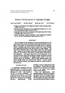
Assessment of the safety conditions of dams is a very challenging task for geotechnical engineers, due to the very big dimensions of these structures and to the presence of different interacting components (foundation, embankment, waterproofing and drainage systems, pipelines and operating machines), so tightly interconnected that evaluating the damage on a single part is impossible without considering the consequences of the whole system. In particular the response of existing earth and rockfill dams under seismic events has nowadays recalled a very large interest due to the increased awareness of the risk connected to seismicity and to the fact that most of these structures are not specifically designed to resist against these stresses. Many dams, constructed for various purposes such as irrigation, energy production, flood control, recreation and earth structures such as highway embankments, fall in earthquake-prone areas (Fig. 1.1).

Fig. 1.1 – Placement of major dams in the world: in red: placement of major dams; in blue: areas of high seismic intensity.

As for the other structures, the safety assessment of earth dams should be investigated with regard to a variety of critical conditions. From the observation of dam behavior during earthquakes occurrences, the following possible failure mechanisms can be identified (Seco e Pinto & Simao, 2010):     

Sliding or shear distortion of embankment or foundation or both; Transverse cracks; Longitudinal cracks; Unacceptable seepage; Liquefaction of dam body or foundation; - 32 -

Chapter 1        

Introduction

Loss of freeboard due to compaction of embankment or foundation; Rupture of underground conduits; Overtopping due to seiches in reservoir; Overtopping due to slides or rockfalls into reservoir; Damages to waterproofing systems in upstream face; Settlements and differential settlements; Slab displacements; Change of water level due to fracture of grout curtain.

The occurrence of these kind of phenomena obviously depends on the typology and the geometry of dam, on the foundation soil, on the type of waterproofing system and on the placement of facilities. For roller-compacted rockfill dams with concrete or bituminous waterproofing face (respectively called CFRD and BFRD), many engineers have argued that these kind of dams are inherently safe against potential seismic damage since the entire embankment is dry and hence earthquake shaking cannot cause pore water pressure buildup and strength degradation. The reservoir water pressure acts externally on the upstream face and hence the entire rockfill mass acts to provide stability (Gazetas & Dakoulas, 1992). In fact in the literature nil or limited have been recorded after strong earthquakes for this kind of dams (Foster, Fell, & Spannagle, 2000). The effects of strong shaking have been acknowledged to manifest primarily in the form of surface cracking (transverse and/or longitudinal cracks) or local slides near the crest of the dam (Ishihara, 2010). For example the Zipingpu dam (Fig. 1.2), a CFRD with height of 156 m and crest length of 663.7 m was shacked during May 12, 2008 by the Wen-Chuan earthquake (magnitude 7.9) in China (Ishihara, 2010). The Zipingpu Dam safely withstood the strong shaking (with peak horizontal accelerations at the crest as high as 2.0g) without collapsing, but high crest settlements of about 74 cm and a downstream horizontal displacement of about 30 cm were observed after the event. A long horizontal offset occurred across the dam about 5m above the water line (the reservoir level was about 830 m u.s.l.) over a length of 600m on the upstream concrete facing. The topmost part of the concrete slab was displaced about 25cm toward the reservoir; in addition, two vertical cracks injured the concrete facing near the left (east) abutment (Fig. 1.3).

- 33 -

Chapter 1

Introduction

Fig. 1.2- Cross section of the Zipingpu dam.

Fig. 1.3 – Backside view of the Zipingpu Dam.

More recently, an extensive inspection carried on after the catastrophic March 11, 2011 Tohoku earthquake (magnitude 9.0) in Japan showed that all the rockfill dams performed well. Most of these showed minor or moderate cracking, but two rockfill dams with bituminous concrete face, the Minamikawa Dam and the Numappara Dam, suffered some cracking in the asphaltic concrete face for a width of about 3mm (Matsumoto, Sasaki, & Ohmachi, 2011) (Fig. 1.4).

- 34 -

Chapter 1

Introduction

Fig. 1.4 - Minamikawa Dam. Cracking of the asphalt concrete face (average width of 3mm).

Therefore, in spite of the overall safety of rockfill dams against collapse due to earthquakes, it is important to limit the occurrence of accidents caused by the lack of functionality of the dam and to prevent secondary effects that can lead to the structure failure. For rockfill dams with concrete or bituminous facing it’s important to guarantee the integrity of the waterproofing element in order to avoid the detrimental effects induced by uncontrolled seepage into the dam body. This may cause the collapse of the structure; as observed for the 71m high Gouhou rockfill dam (Zhang & Chen, 2006) failure was induced by the internal erosion caused by seepage consequent to construction defects of the concrete facing. Furthermore, excessive settlements of the dam’s crest may be not compatible with the functionality of the dam and may be impossible to be restored. In the worst case, they may cause the overtopping of the reservoir water or the inability to adjust the reservoir level due to the damage of the water regulation facilities. 1.2

Scope of work

The prevention of the phenomena described above phenomena is a key aspect for the design of modern, roller-compacted rockfill dams. This goal should be kept for the rehabilitation of existing old dams, often designed with simplified methods and out-of-date codes. For these latter structures a new check should be performed with up to date criteria. The evaluation of the seismic safety for this kind of structures, regardless of the type of construction, must be based on the assessment of the seismic risk, intended as the product of the hazard of the seismic event, the structure vulnerability and the exposition (or potential downstream risk). In Italy the most of the existing dams have been built between 50’s and 90’s. Among them, about 10% are rockfill dams with central clay core or bituminous concrete - 35 -

Chapter 1

Introduction

waterproofing face. The seismic hazard associated to these dams is high, mostly due to the high seismicity characterizing the whole Italian territory; the vulnerability may be also high because of the use of old design criteria; the exposition is generally high due to the presence of urban areas near the reservoirs. This kind of structures, designed with a poor knowledge on their seismic behavior, with limited calculation tools, or without considering seismic actions since the dam’s site was assumed aseismic, could be not respondent to the acceptability criteria fixed in newer codes. The challenge of this research is to investigate the aspects able to influence the seismic response of rockfill dams with bituminous concrete face with the aim of defining a comprehensive procedure, to design countermeasures improving the safety of these structures. However, this very appealing goal requires that the whole building process of the dam (excavation, foundation reinforcement and/or waterproofing, origin and placement of materials) is perfectly reconstructed and sufficiently accurate experimental investigations are available or ad hoc performed. For this purpose, a deep literature analysis has been conducted where the factors that influences the seismic behavior of rockfill dams are identified. Common and uncommon approaches for the seismic analysis of these structures are analyzed. Then, a general review of modern approaches adopted for the seismic assessment of geotechnical structures has been presented. After, a case study has been described and the seismic behavior has been evaluated. A comprehensive analysis of constitutive models available for granular soils has been conducted, in order to select the most suitable model for the studied case. The choice has been made taking into account both the necessity of a constitutive model able to simulate as close as possible the cyclic behavior of soils, and the availability of sufficient data for an effective calibration of the model itself. Results obtained with a 2D and 3D modelling have been critically discussed analyzed in order to verify the seismic safety of the rockfill dam.

- 36 -

Chapter 2 Seismic analysis of rockfill dams: literature review

Chapter 2 2.1

Seismic analysis of rockfill dams: literature review

Factors affecting the response of rockfill dams

To make a realistic prediction of the response of an earth dam to a particular earthquake shaking, careful consideration must be given to the potential effects of the following major phenomena/factors (Gazetas, 1987) (Gazetas & Dakoulas, 1992):        

characteristics of the seismic input; dependence of rockfill stiffness on confining pressure; nonlinear-inelastic material behavior of rockfill; 3D canyon geometry; flexibility of supporting canyon and presence of underlying alluvia; asynchronous excitation; liquefaction of dam’s soil or underlying alluvia; other factors.

Depending on the particular situation, one or more of these phenomena may have an appreciable influence on the response of the dam and will thereby dictate the proper method of analysis. 2.1.1

Characteristics of the seismic input

The seismic input is one of the most important factors influencing the behavior of rockfill dams, in particular the amplitude, the duration and the frequency content are the key factors affecting the response (Kramer, 1996). Known that dams are flexible bodies, high seismic amplitudes may induce high peak accelerations due to the amplification effect induced by dam’s body and, hence, high displacements. The duration of strong motion also can have a strong influence on earthquake damage. Many physical processes, such as the degradation of stiffness and strength of certain types of materials and the buildup of pore water pressures in loose, saturated sands, are sensitive to the number of load or stress reversals that occur during an earthquake. A motion of short duration could not produce enough load reversals for damaging response to build up in a structure, even if the amplitude of the motion is high. On the other hand, a motion with moderate amplitude but long duration could produce enough load reversals to cause substantial damage. Earthquakes produces complicated loading histories with motion components spanning over a broad range of frequencies. It’s known that the dynamic response of compliant objects, be they buildings, such as bridges, slopes, or soil deposits, - 38 -

Chapter 2


is very sensitive to the frequencies at which they are forced; in particular, if the frequency content of the seismic motion (typically expressed in terms of Fourier spectra or response spectra) is closer to the dam’s dominant oscillation frequency, resonance effects may arise with deleterious effects for the overall stability of the embankment. 2.1.2

Dependence of rockfill stiffness on confining pressure.

The material inhomogeneity due to the dependence of soil stiffness on the static confining pressure has been verified by numerous laboratory investigations. It has been recognized to affect the dynamic response of earth dams causing higher acceleration values and displacements at the crest. First studies (Dakoulas & Gazetas, 1985) (1986) have used the inhomogeneous “shear-beam” approach (for method description, see par. 2.2.3) considering 2D ideal dams on a rigid base and expressing the shear modulus in the form of 𝐺𝐺 = 𝐺𝐺𝑏𝑏 (𝑧𝑧⁄𝐻𝐻 )𝑚𝑚 where Gb is the average shear modulus at the base, H is the height of the dam and m is a coefficient depending on the material and the dam’s geometry. Parametric results showed that increasing m (i.e., inhomogeneity) leads to a sharper attenuation of mode displacements (Fig. 2.1b), almost identical fundamental frequency and closer spaced higher natural frequencies (Fig. 2.1a). Also, higher displacement and acceleration values are evident at all resonances, together with greater relative importance of the higher modes on the acceleration response (Fig. 2.2), and occurrence of maximum values of shear-strain modal shapes closer to the crest (Fig. 2.1c). The same analysis, performed on a 120 m tall ideal dam, subjected to the Taft 1952 NE component recorded motion and modeled as a shear beam (Gazetas, 1987) showed that, at the top quarter of the dam, peak acceleration and, to a less extent, peak displacements, are sensitive to m (increase with increasing m) instead of shear stresses that are hardly influenced by m. As a result, shear strains, being at all times inversely proportional to G(z), are strongly affected by inhomogeneity (Fig. 2.3).

- 39 -

Chapter 2


(a)

(b)

(c)

Fig. 2.1 – Effect of modulus inhomogeneity parameter m on natural periods (a), modal displacements (b) and modal strain participation factors (c) (Gazetas, 1987).

- 40 -

Chapter 2


Fig. 2.2 - Effect of m on steady-state crest amplification function for “rigid rock” case (Gazetas, 1987).

2.1.3

Nonlinear-inelastic material behavior of rockfill.

The foregoing conclusions have been obtained considering very weak seismic ground shaking that induces very small shear strain. In this case the constituent materials behave in a quasi-linear elastic manner. Nonlinear elastic soil behavior during strong ground shaking may even reverse some of the observed trends. Considering the same 120 m tall dam defined before and the same seismic input, the dependency of the stiffness on the strain level was considered assuming hyperbolic average stress-average strain backbone relationship for the soil (dependent on the strain level γ) (Gazetas, 1987): 𝜏𝜏 = 𝜏𝜏(𝑧𝑧, 𝛾𝛾) = 𝐺𝐺(𝑧𝑧)

𝛾𝛾 𝛾𝛾 1 + �𝛾𝛾𝑟𝑟

(1)

With G(z) = low strain elastic modulus = Gb(z/H)m; and γr = reference strain = τmax(z)/G(z). The same results of Fig. 2.3 are reported in Fig. 2.4 considering three different values of m (0; 1/3; 2/3) and two different values of γr (0.003; 0.0013). It can be seen that strong nonlinear action (smaller γr) leads to substantial reduced amplification with respect to the linear elastic analysis. Moreover, the increased inhomogeneity (larger m) becomes a secondary effect with respect to the nonlinearity of soil. On the other hand, despite the inelastic action during the nonlinear analysis, the distribution of shear strains essentially retain its linear-elastic shape. On the contrary, the differences between peak - 41 -

Chapter 2


Fig. 2.3 – Effect of degree of inhomogeneity on distribution with depth of peak seismic response variables for m=0; 1/3; 2/3 (Gazetas, 1987).

Fig. 2.4 – For a given excitation, with increasing nonlinear inelastic action: (a) the near-crest peak accelerations decrease and the effects of inhomogeneity tend to diminish; but (b) the peak shear strain distributions remain nearly unchanged, both in magnitude and shape (Gazetas, 1987).

- 42 -

Chapter 2


relative displacements, increases with increasing magnitude of nonlinearity. In general, nonlinearity induced by stronger earthquakes have a beneficial role because it produces a higher damping. It tends to elongate the fundamental dam period which might thus fall well outside the significant period range of ground motion, thus avoiding resonance effects; it also tends to destroy the higher frequency components of recorded ground motions. 2.1.4

3D canyon geometry.

With regard to the effect of geometry, the assumption of plane-strain condition in the analysis of rockfill dams is exactly valid only for infinitely long dams subjected to synchronous lateral base motion. For dams built in narrow valleys, as is frequently the case of rockfill dams built in mountainous regions, the presence of relatively rigid abutments creates a 3D stiffening effect. This condition produces an increase of the natural frequencies; modal displacements tend to become sharper as the canyon becomes narrower. First comparisons between two dimensional and three-dimensional analyses of earth dams have been reported by Hatanaka (1955) and Ambraseys (1960) who studied the seismic behavior of a two dimensional shear wedge located in a rectangular canyon and concluded that for length to height ratios of four or greater, the fundamental longitudinal period of vibration was approximately equal (within 10%) to that of an infinitely long dam. Results of different analyses for different canyon shapes are reported in Fig. 2.5 where T1,∞ represents the natural period of an infinitely long dam under plane deformation, and L/H is the aspect ratio. The figure illustrates that the stiffening effect of narrow canyon geometries on the first natural mode is particularly important for aspect ratios smaller than 3. The results are valid for homogeneous dams. However, for a given aspect ratio and canyon shape, the ratio T1/T1∞ is hardly influenced by inhomogeneity due to the dependence of soil stiffness on the static confining pressure (see par. 2.1.2 ) and hence results of Fig. 2.5 may be used for estimating the canyon effects with any type of dam. With regard to the acceleration values, midcrest “rigid-rock” amplification function for a dam in a semi-cylindrical canyon is compared with the one obtained from a 1D shear-beam analysis for the mid-section of the same dam (Fig. 2.6a). It is evident that, in addition to the prediction of lower natural frequencies, the plane model underpredicts both the amplification at first resonance and the relative importance of higher resonance frequencies that, for dams built in narrow canyons, give an important contribute to the dynamic response. The effect of different canyon shapes (Fig. 2.6b) exhibits a consistent - 43 -

Chapter 2


trend and reveals that the amplification value at first resonance is practically independent of the canyon shape. An interesting case history which provides field evidence to the results showed in Fig. 2.7 regards the 76m tall Ririe dam, built in a narrow canyon (Mejia, Seed, & Lysmer, 1982). Fig. 2.7 shows the amplification ratio between the Fourier spectra at the crest and abutment acceleration records versus frequency, after the 1983 Mt. Borah earthquake. The theoretical curve also plotted was computed from a 2D finite element model of the midsection of the dam. It can be seen that the higher mode amplitudes of the 3D reality exceed those of 2D analysis in a way similar to that suggested by the theoretical 3D vs 2D plot of Fig. 2.6. In all the above examples, the stress-strain behavior of soil was considered linear elastic. Generally speaking, soil nonlinearity tends to reduce peak accelerations due to increased hysteretic dissipation of wave energy and destruction of potential resonances. Additionally the high frequency, high amplitude acceleration components which tend to generate in inhomogeneous 3D dams, tend to be flattened by the decay of stiffness.

Fig. 2.5 – Effect of canyon geometry on the fundamental natural period (Gazetas & Dakoulas, 1992).

- 44 -

Chapter 2


(a)

(b)

Fig. 2.6 – Steady-state response to harmonic base excitation: (a) semi-cylindrical dam determined from 3-dimensional and from plane shear-beam analysis; (b) effect of canyon shape on midcrest amplification function. (Gazetas & Dakoulas, 1992).

- 45 -

Chapter 2


Fig. 2.7 - Crest-to-abutment amplification spectrum of the Ririe Dam in the 1983 Mt. Borah earthquake. The theoretical spectrum (dotted line) was computed with a 2D plane-strain model, in which the moduli were selected to account for the apparent stiffening effect of the narrow canyon. (Gazetas & Dakoulas, 1992).

2.1.5

Flexibility of the supporting canyon and presence of underlying alluvia.

A major assumption in most of the studies is that every point at the interface of the dam and its surrounding medium experiences identical motion (i.e., the base of the dam moves as rigid body). This assumption neglects two potentially important effects: (1) the interaction between the dam and foundation; (2) the destructive or constructive wave interference in the dam due to phase and amplitude differences in the incoming wave motion. Considering the first effect, there’s field evidence of energy dissipation through wave radiation during forced vibration of dams (Abdel Ghaffar & Scott, 1981). By considering deformable canyons of simple shapes, Dakoulas (1993) and Dakoulas & Hsu (1995) found that the amplitude of the dam response strongly depends on the impedance ratio between the dam and the canyon impedances (α = ρC/ ρrCr were ρ;C and ρr;Cr are the density and the shear wave velocity respectively of the dam and the foundation soil). As can be observed in Fig. 2.8, increasing the impedance ratio (i.e., reducing the stiffness of foundation) induces a smoothing effect of the amplification function at the mid-crest of the dam, with consequent lower acceleration - 46 -

Chapter 2


values. Therefore, the presence of a flexible canyon-rock tends to reduce the amplification peaks at resonance.

Fig. 2.8 - Effect of rigidity contrast (impedance) ratioα=ρC/ρ r C r on crest amplification for inhomogeneity parameter m = 2/3 (Gazetas, 1987).

2.1.6

Asynchronous excitation

The previously discussed 3D studies of the seismic response of dams have invariably assumed that the points at the dam-valley interface experience identical and synchronous oscillations and hence that a single accelerogram is sufficient to describe the excitation. In reality, however, seismic shaking is the result of a multitude of body and surface waves striking at various angles and creating reflection and diffraction phenomena. The resulting oscillations differ in phase, amplitude, and perhaps also in frequency content, from point to point along the dam-valley interface. The development of asynchronous motions in earth dams can be related to the features of the input motion (frequency content, amplitude and duration) and to the features of the dam embankment (mainly: geometry, stiffness and damping of the construction soils). In general, asynchronism tends to increase when the higher vibration modes of the dam embankment are excited. This is likely to occur when the seismic signal is rich in high frequencies or the natural frequencies of the dam are relatively low. This is the case of very high dams or embankments made of very deformable materials. Various field examples can be found in the literature (Bilotta, Pagano, & Sica, 2010). - 47 -

Chapter 2


The few attempts produced in the literature to address this problem (Dakoulas et al., 1992; Dakoulas, 1993; (Papalou & Bielak, 2001) (Papalou & Bielak, 2004), have shown a reduction of the dam acceleration compared to the case when seismic input was assumed to be synchronous. 2.1.7

Liquefaction of dam’s soil or underlying alluvia

On bituminous concrete faced rockfill dams, the presence of the waterproofing face guarantees that the entire embankment is dry and hence earthquake shaking cannot cause pore water pressure buildup and strength degradation. The liquefaction phenomenon may affect the underlying alluvia if it’s composed by loose, saturated sand. In saturated loose and medium dense granular materials pore pressure buildup during the ground shaking affect the resistance, and consequently the stability of the embankment under the cyclic loading, during and following the seismic event. Two well-known events due to buildup of pore pressures during earthquakes are the Sheffield Dam failure (Seed, Lee, & Idriss, 1969) and the major slide occurred in the upstream slope of the Lower Sam Fernando Dam (Seed, Pyke, & Martin , 1975). An analysis technique is required which takes into account the pore pressures generated during the cyclic loading and their effects on the stability of the earth structure. A series of methods have been developed by different authors ( (Seed, Martin, & Lysmer, 1976) (Ishihara, Tatsuoka, & Yasuda, 1975) (Finn, Lee, Maartman, & Lo, 1978) in order to include considerations of pore pressure redistribution during and following the earthquake shaking. 2.1.8

Other factors

The reservoir water acts as a load on the upstream face, inducing a stiffening effect due to the increased confining pressure of dam’s soil and contributes to increasing the lateral deformations in the downstream direction, when plastic straining occurs. In general, hydrodynamic effects can be safely ignored in estimating the seismic response of rockfill dams (Bureau, Volpe, Roth, & Udaka, 1985). The stiffness waterproofing membrane, made in general with concrete or bitumen, generally does not affect the dynamic behavior of rockfill dams (Uddin, 1999). All the aforementioned factors plays a different role in dynamic behavior of rockfill dams, depending on the type of dam and on the magnitude of seismic event. For stiff, modern dams subjected to ground shaking having peak - 48 -

Chapter 2


acceleration of the order of 0.2g or less, soil nonlinearity becomes less important respect to the effect induced by the geometry, the inhomogeneity and the dam-foundation interaction. Thus, a preliminary assessment of the importance of each of these factors is a recommended first step, before starting comprehensive sophisticated numerical models. 2.2

Dynamic analysis methods: historical review

All the methodologies developed over the years for the dynamic analysis of earth and rockfill dam can be summarized as follows (Seco e Pinto & Simao, 2010):  pseudo-static analyses;  simplified procedures to assess deformations;  dynamic analyses. This kind of sorting follows the historical development of knowledge in geotechnical earthquake engineering from 1940 to nowadays. 2.2.1

Pseudo-static analyses

In the early stages of geotechnical earthquake engineering, the standard seismic method for earth dams (Terzaghi, 1950) was based on the erroneous assumption that dams were absolutely rigid bodies fixed on their foundation and thus experiencing a uniform acceleration equal to the underlain ground acceleration. The latter was specified in seismic codes in terms of a single peak value and was taken as acting pseudo-statically in one direction, giving rise to a horizontal inertia-like force applied in the barycenter of a potential sliding mass and determined as the product of the weight of the trial unstable mass and a seismic coefficient related to the peak acceleration (Fig. 2.9).

Fig. 2.9 – Pseudo static approach: forces acting on a rigid wedge sliding on a plan surface (Terzaghi, 1950).

- 49 -

Chapter 2


One potential drawback of this procedure was that the horizontal inertia forces do not act permanently and in one direction but rather fluctuate rapidly in both magnitude and direction; thus, even if the factor of safety dropped momentarily below unity the slope would not necessarily experience a gross instability but might merely undergo some permanent deformations (settlements). Embankments made of granular material rarely behave as rigid bodies. In order to take into account the amplification of the seismic motion from the base to the dam’s crest, Ambraseys (1960) analyzed the response of dams with different geometries assuming a viscoelastic behavior. As a result of such analysis, provided correlations between the dam’s height and the seismic coefficient (Fig. 2.10).

Fig. 2.10 – Variation of the seismic coefficient k with dam’s height (Ambraseys N. , 1960).

Seed and Martin (1966) suggested a new method to predict dynamic seismic forces and their variations with time. They investigated viscoelastic response behavior of dams idealized as an infinitely long triangular cross-section with uniform and homogenous material properties under El Centro earthquake - 50 -

Chapter 2


accelerations. Assuming triangular wedge-shaped sliding masses, an average seismic coefficient, kav is defined for the trial wedge as: 𝑘𝑘𝑎𝑎𝑎𝑎 =

1 ∙ � 𝑚𝑚(𝑦𝑦)𝑢𝑢𝑎𝑎̈ (𝑦𝑦) 𝑊𝑊

(2)

where W is the weight of the sliding mass, m is the mass of an incremental slice of the sliding mass, ua is the absolute acceleration of the slice at the instant under consideration and y is the distance to the incremental slice from the top of the dam, as shown in Fig. 2.11.

Fig. 2.11 – Concept of average seismic coefficient (Seed & Martin, 1966).

Despite several attempts to improve the method, many other factors affecting the global stability of the dam are neglected, like the frequency content of the earthquake, the inhomogeneity of the dam’s soil, the asynchronous seismic input. Furthermore, the method accounts for slope instability as the only possible mode of failure and it was not considered likely to occur unless the pseudo-static factor of safety of the trial slide mass occurred to be smaller than unity. It’s well known that several other types of seismic damages may happen in earth dams, but the most important shortcoming is that the pseudo-static approach does not give any idea whether plastic deformations are expected to occur during earthquake or not. 2.2.2

Simplified procedures to assess deformations

In order to assess the permanent displacements of embankments under cyclic loading, Newmark (1965) proposed a new method based on the analysis of a rigid block sliding on a plane. The fundamental principle is depicted in Fig. 2.12. It is assumed that the potential sliding mass .behaves like a rigid block and the shear resistance is assumed as constant. When the inertial force induced by the earthquake motion reaches values such that destabilizing forces (static and dynamic) exceed frictional resistances, the block starts sliding. The first displacements occurs when the induced acceleration exceeds a threshold value - 51 -

Chapter 2


defined as “critical acceleration ay”. Pointing with “kv” the critical seismic coefficient, the critical acceleration is ay = ky g. The yield acceleration can be readily determined using conventional limit equilibrium methods, i.e. by calculating the inertial forces required to produce factor of safety against block sliding lower than 1.0. Several failure surfaces should be analyzed in addition to that producing the lowest static factor of safety. Irreversible displacements are calculated by double integration of the acceleration, when it exceeds the critical one. The sum of partial displacements provides the total final displacement of the slope. One of the major drawbacks of the Newmark approach is that, due to the rigid mass assumption, the acceleration induced by seismic motion is the same in every point of the dam, i.e. coincident with the base acceleration. As observed before, dams are flexible bodies, hence seismic motion induces different inertial forces in any point of the dam, depending on the type of seismic input (duration, amplitude, frequency content) and the material stiffness. In these conditions, the rigid block assumption leads to an overestimation of the irreversible displacements induced by seismic motion.

Fig. 2.12 – Integration of effective acceleration time-history to determine velocities and displacements (Newmark, 1965).

- 52 -

Chapter 2


To take into account the spatial and temporal variability of seismic acceleration into the dam’s body, Makdisi and Seed (1978) suggested to calculate a medium acceleration along the potential slippage surface with the procedure proposed by Chopra (1966) by finite element method. Typical variation of effective peak acceleration on a sliding mass as obtained from the dynamic response of embankments, kmax, with the depth of the dam is depicted in Fig. 2.13, divided by the maximum crest acceleration umax. (Hynes-Griffin & Franklin, 1984) carried out sliding block analyses by employing 348 horizontal earthquake records and six synthetic records. They summarized the results in terms of variation of the computed permanent displacements, u, with the ratio N/A, where N is the critical acceleration and A is the peak earthquake acceleration, as shown in Fig. 2.14. Similar computations carried out by Makdisi & Seed (1978), Sarma (1975), and Ambraseys (1973) for earthquakes with magnitudes of about 6.5, produced results are shown in Fig. 2.15. In Fig. 2.15, km represents the effective peak acceleration as a fraction of the peak acceleration developed at the crest of the embankment, and ky is the yield (or critical) acceleration. From charts such as Fig. 2.14 and Fig. 2.15, the order of magnitude of the potential displacements occurring during shaking of embankments can be estimated.

Fig. 2.13 – Variation of “maximum acceleration ratio” with depth of sliding mass (Makdisi & Seed, Simplified procedure for estimating dam and embankment earthquake-induced deformations, 1978).

- 53 -

Chapter 2


Fig. 2.14 - Permanent displacement u vs N/A, based on 348 horizontal components and six synthetic accelerograms (Hynes-Griffin & Franklin, 1984).

Fig. 2.15 – Computed displacements of embankment dams subjected to magnitude 6.5 earthquakes having little or no loss of strength due to earthquake-induced deformations (Seed H. , 1979).

- 54 -

Chapter 2


Despite the improvements from different authors, such simplified methods are useful only for a preliminary assessment of the safety of dams and in cases with limited nonlinear behavior of soil (weak earthquake motions) due to the simplified soil’s behavior. Also these methods provide only overall horizontal displacements of the trial sliding wedge, without any information about the loss of the freeboard and the overall performance of the dam and facilities. 2.2.3

Dynamic analyses.

At the earlier stages of dynamic analyses, one of the first approaches to the dynamic analysis of two-dimensional earth structures was the shear beam analysis (Mononobe, 1936) (Fig. 2.16). In its basic original form, the shear beam model was based on the following major simplifying assumptions: (a) only horizontal lateral displacements and simple shearing deformations take place; (b) displacements and shear stresses and strains are uniformly distributed along horizontal planes across the dam; (c) the dam consists of a homogeneous material which behaves as a linear viscoelastic solid and is described by a constant shear modulus, damping ratio, and mass density; (d) the dam is either infinitely long or built in a rectangular canyon and is subjected to a synchronous rigid base lateral motion. The approach has then been verified and extended to cover a variety of conditions in order to account for the inhomogeneity of dam’s soil and the 3D effects for dams build in narrow canyons. Different closed form relations have been defined in order to calculate fundamental periods, modal displacements and amplification functions (Gazetas, 1987). This method, still simplified, does not take into account the complex nonlinear behavior of the material, including the necessary assumptions (a) and (b) for shear model, which in some cases may be too restrictive.

Fig. 2.16 – The shear beam model.

- 55 -

Chapter 2


After 1960 the first implementation and subsequent widespread use of the finite-element and finite difference methods appeared in studying the seismic response of earth dams. The popularity of these new methods growed basically due to two factors: (a) its capability for handling any number of zones with different materials, whereas the shear beam model assumed that the elastic properties of the dam could be represented by an average value: and (b) its capability of rationally reproducing the 2D and 3D dynamic stress and displacements field during earthquake shaking, whereas the simplifying assumption of uniform horizontal shear stresses in shear-beam analyses seemed to violate physical requirement of vanishing stresses on the two faces of the dam. The development of new numerical capabilities gave the start for the growth of new dynamic approaches such as equivalent linear approach and nonlinear approach. For the equivalent linear approach (Idriss, Lysmer, Hwang, & Seed, 1983) an equivalent linear analysis is performed in an iterative way. The method utilizes results from laboratory tests in the form of shear modulus and damping ratio versus sinusoidal shear strain amplitude (Fig. 2.17). A set of moduli and damping ratios is initially assumed and a series of linear analyses is conducted, with each calculation using soil moduli and damping ratios compatible with the levels of shear strain calculated in the previous step. To select modulus and damping ratio for each iteration, an “equivalent” effective strain amplitude is estimated as a fraction (usually 2/3) of the peak shear strains.

- 56 -

Chapter 2


(a)

(b)

(b)

Fig. 2.17 – Variation of shear modulus (a) and damping ratio (b) with shear strain amplitude (Rollins, Evans, Diehl, & Daily, 1998).

Clearly, the arbitrary selection of the last factor is a major drawback of the method, also, the method is empirical and its convergence to the correct answer cannot be proved theoretically. For moderately strong levels of shaking the - 57 -

Chapter 2


peak response values seem reasonable, while the response to very strong excitation may be overestimated or even underestimated. Since the method is essentially linear during each iteration, there’s a tendency for spurious resonances to develop and thereby to exaggerate the response. Finally, the method cannot provide information on permanent displacements ad deformations, since it’s basically an elastic method. Hence, there’s the need to develop separate procedures for assessing residual and sliding displacement, e.g. by using the aforementioned Newmark concept. This method is widely used for evaluating the local site seismic response and has been implemented in numerous 1D and 2D codes like Shake91 (Schnabel, Lysmer, & Seed, 1972) and QUAD4M (Hudson, Beikae, & Idriss, 1994). Nonlinear approaches, such as these involving soil nonlinearity at different degree of complexities, are suitable for the prediction of permanent displacements of dams and of the complete performance of these structures. Different possible nonlinear methods are described below. The simplified nonlinear method (Gazetas, 1987) is an approximate method that attempts to overcome in a simple way the two main limitations of equivalent linear method: the arbitrary definition of equivalent shear strain amplitude and the spurious resonance effect. In this method soil moduli and damping ratios can be updated at various time intervals so as to be consistent with the root mean squared values γrms(t) of the shear strain during the same interval. In other words, updating of the soil parameters is enforced at several points along the time axis, in contrast with assigning a single value, to stepwise update the equivalent linear scheme. The Layered Inelastic Shear-Beam (LISB) method attempts to combine the simplicity and efficiency of the one-dimensional shear-beam type of analysis with the versatility of (plane-strain) finite-element in handling zones of different material and nonlinear element behavior. The method involves two stages. In stage I, the dam is discretized into finite elements and is subjected to horizontal static inertia-like forces. The nonlinear deformations of the dam are computed using the best available plane-strain code, while the applied horizontal forces are gradually increased until large enough strains develop in most elements of the dam. This static analysis provides for each horizontal layer (super-element) the backbone curve relating the total horizontal shear force and average horizontal layer distortion; this backbone curve together with the extended Masing criterion provides the complete hysteretic constitutive relation required for the dynamic analysis in stage II. In the second stage the dam is discretized as a one-dimensional layered triangular shear- 58 -

Chapter 2


beam and the dynamic response of the dam is computed using nonlinear shear beam formulations. The approximate 2D nonlinear effective stress analysis (Finn, 1988) extends the 1D hyperbolic Masing model of cyclic behavior in simple shear to approximately account for inelastic soil behavior in two dimensions. The method can handle transient and residual pore water pressures generated and diffused during the shaking, as well as volumetric compaction due to shear. The model for residual pore water pressures (which arise due to plastic deformations) is a straightforward extension of the 1D Martin-Finn-Seed (Martin, Finn, & Seed, 1975) model that has been widely used for siteamplification and liquefaction studies. Applications of this method have been published for embankments and related earth structures. Tested against centrifuge-measured seismic histories of deformations and residual pore water pressures the method seems capable of capturing all the important features of the response with very good engineering accuracy and according to Finn, (Finn, 1988) at a substantially-reduced computational cost in comparison with more rigorous plasticity based models. The rigorous plasticity based FE and FD methods utilize plasticity models of soil behavior in a FE formulation. For example, Prevost and co-workers discretize the dam in eight-node isoparametric “brick” elements or four-node isoparametric elements for three and two dimensions, respectively. The formulation can handle either one of the three orthogonal components of the seismic excitation (upstream-downstream, vertical, and longitudinal). The hysteretic stress-strain behavior of the dam material is modeled by using multisurface kinematic plasticity theory, and a symmetric backbone curve. As a result a Masing-type hysteretic behavior is generated. The time integration of the semi-discrete finite element equations is performed by an implicit-explicit predictor-multi-corrector algorithm, based on the Newmark method. The general validity of the method has been checked against the recorded response of the Santa Felicia (Prevost, Abdel-Ghaffar, & Lacy, 1985) and of the Long Valley dam (Griffiths & Prevost, 1988). Both 2D and 3D analyses were performed in these studies. However, the finite element mesh used in such analyses seems to be very coarse, especially in 3D studies, due to the very substantial computational requirements of the method. It is quite likely that high frequency components are artificially filtered out or at least reduced as they propagate through a coarse mesh; this may especially affect the accelerations computed for the crest zone.

- 59 -

Chapter 2


With the progress of computational capability, this last nonlinear method has been the most used method to assess the performance of new and existing rockfill dams. It takes into account not only the stress-strain behavior of soils, but also the interaction with the pore water and the possibility of liquefaction phenomena.

- 60 -

Chapter 3 Procedure for the assessment of existing rockfill dams

Chapter 3

Procedure for the assessment of existing rockfill dams

In the last years the general evolution of the structural design criteria, and the major importance given to the seismic behavior of existing buildings, have extended the objectives of the seismic analysis. Safety against collapse remains the most important objective, but performance in terms of functionality and economy have assumed a central role in the design criteria. Therefore several authors have discussed the need of improving the current earthquake resistant design methods in order not only to avoid the collapse for destructive earthquake, but also to limit the damage for moderate earthquakes. Moving from a simple force-strength approach, the new design philosophy tends to multi-level probabilistic structural performance criteria called Performance Based Seismic Design (PBSD). In a broad sense, PBSD can be understood as a design criteria whose goal is the achievement of specified performance targets when the structure is subjected to a defined seismic input. The specified performance target could be a level of displacement, level of stress, maximum acceleration, mobilized strength, or a limit state. The use of PBSD is definitely less widespread in geotechnical engineering than in structural engineering. Nevertheless, from the 60s, the earthquake geotechnical community is applying analytical methods for predicting permanent displacements in earth structures, which is basically a performance criterion as opposed to the classical concept of limit equilibrium. From the middle 90s, geotechnical engineers from different countries have promoted the development of PBSD methods, but the application to earth structures, such as earth and rockfill dams, has been pursued only in limited cases. Among various factors to be considered, significant uncertainties exist in the definition of performance targets, since these structures include different components (foundation, embankment, waterproofing and drainage systems, pipelines and operating machines), so tightly interconnected that evaluating the consequences (and/or the repair costs) of a damage on a single part is impossible without considering the whole system. Furthermore, it is widely acknowledged that prediction of the seismic response of earth structures, even with the most modern numerical tools, is not easy due to a number of reasons including three dimensional geometries (Prevost, Abdel-Ghaffar, & Lacy, 1985), nonlinear irreversible stress-strain response of the constituent materials (Modoni, Koseki, & Anh Dan, 2011), interaction between different materials, e.g. core-shell interaction in zoned dams, or embankment body-bituminous facing for rockfill dams. Examples of predictions on dams inspired to the principles of PBSD can be found in the literature (Sica & Pagano, 2009) (Tani, Tsukuni, & Shiomi, 2009).

- 62 -

Chapter 3


In principle, PBSD analyses can be performed even on existing dams, i.e. designed with conventional methods, in order to predict their performance under a variety of events and, eventually, plan countermeasures aimed to optimize their financial management. However, this very appealing goal requires that the whole construction process (excavation, foundation reinforcement and/or waterproofing, origin and placement of materials) is reconstructed with sufficient accuracy and that experimental investigations are available or ad hoc performed. Nowadays, a possible procedure for the assessment of seismic safety of existing rockfill dams has not been defined yet, but after the observation of literature data regarding damages of existing dams, and after the review of traditional and new analysis methods, the procedure proposed for the application of PBSD on existing rockfill dams could be defined into the following four steps:  definition of performance objectives;  selection of seismic inputs  numerical model of the dam;  geometry building process;  selection and calibration of constitutive model;  evaluation of the dam’s response. 3.1

Definition of performance objectives

The definition of adequate performance objectives consists in a clear statement of limit conditions to be avoided with prescribed levels of probability (or return periods). Generally, for new structures, this objective can be achieved only after a cost benefit analysis depending on the type and importance of the structure, the consequences of damage and the cost for repair of the structure. Selection of performance objectives for existing rockfill dams is not straightforward but depends on the type of structure to be studied. International codes and, more recently, Italian codes (M.LL.PP., 2008) have introduced PBSD concepts for the design of structures. With regard to existing earth and masonry dams, specific guidelines have been proposed (C.S.LL.PP., 2007) (C.S.LL.PP., 2009) which give a more clear definition of performance objectives with the identification of different limit states. In particular, a correspondence is established between limit states defined in the EC8 and limit conditions not to be attained by the dam’s response. Furthermore, each of these conditions is related to a tolerated probability of failure Pr which, according to - 63 -

Chapter 3


the expected life of the dam, gives the return periods to be assigned in the analysis (Table 3.1), according to the following relation: 𝑇𝑇𝑅𝑅 = −

𝑉𝑉𝑅𝑅 (1 − ln 𝑃𝑃𝑉𝑉𝑅𝑅 )

(3)

Where VR is the reference period, defined by Italian regulations as the product between expected life of the dam VN and the usage coefficient CU. For every limit state, a corresponding limit condition is defined, such limit condition must not be attained in order to satisfy the corresponding limit state. The OLS and DLS are defined serviceability limit states and, for these limit states, the dam must retain all the functionalities. The LLS and CLS are defined ultimate limit states and for these limit states the dam may suffer damages but must be able to maintain its capability to retain water (no collapse) and to control the reservoir level.

Limit state

Corresponding limit condition

Operational limit state (OLS)

Facilities suffer limited damages but the reservoir level can be controlled Slopes suffer local instabilities but the stability of the embankment is ensured. Facilities are damaged without uncontrolled release of water Cracks or excessive deformations of embankment and/or foundation cause uncontrolled seepage and/or overtopping. Damage of facilities affects the capability to control the reservoir level Global instability or liquefaction of embankment and foundation

Damage limit state (DLS)

Life safety limit state (LLS)

Collapse limit state (CLS)

PVR (%) 81

63

10

5

Table 3.1 – Limit conditions and tolerable probability of failures for dams

For the seismic safety assessment of existing rockfill dams it has been considered only one serviceability limit state (DLS) and one ultimate limit state (CLS).

- 64 -

Chapter 3 3.2


Selection of seismic inputs

A correct selection of seismic inputs requires a seismic hazard analysis to be performed in order to define PGAs and response spectra for the site under investigation (Kramer, 1996), i.e. quantitative estimation of the ground shaking hazards at a particular site. Seismic hazards may be given deterministically, assuming particular earthquake scenarios, or probabilistically, considering uncertainties in earthquake intensity, location, and time of recurrence. 3.2.1

Deterministic seismic hazard analysis

In the past, the use of deterministic seismic hazard analysis (DSHA) was prevalent. It involves the assumption of a particular seismic scenario upon which a ground motion hazard evaluation is based. The scenario is postulated for a specified location by this four-step process (Fig. 3.1): 1. Identification and characterization of all earthquake sources capable of producing significant ground motion in the studied site. Source characterization includes definition of position and potential of the earthquake. 2. Selection of a source to site distance parameter for each source zone. In most DSHAs, the shortest distance between the source zone and the site of interest is selected. Epicentral or hypocentral distance, depending on the measure of distance of the predictive relationships used in the following step, can be taken. 3. Selection of the earthquake expected to produce the strongest level of shaking, based on relevant ground motion parameter. The selection is made by comparing the levels of shaking produced by earthquakes at the distances identified in step 2. The controlling earthquake is described in terms of its intensity (usually expressed as magnitude) and distance from site. 4. The hazard at the site is formally defined, in terms of ground motions produced at the site by the controlling earthquake. Hazard is usually described by one or more ground motion parameters obtained from predictive relationships. Peak acceleration, peak velocity and response spectrum ordinates are commonly used to characterize the seismic hazards.

- 65 -

Chapter 3


Fig. 3.1 – Four steps of a deterministic seismic hazard analysis (Kramer, 1996).

When applied to structures for which failure could have catastrophic consequences, such as large dams, DSHA provides a straightforward framework for evaluation of worst-case ground motions. However, it provides no information on:  the probability of occurrence of the controlling earthquake;  the probability of occurrence in the site where it is assumed to occur;  the level of shaking that might be expected during a finite period of time (such as the useful lifetime of a particular structure);  the effects of uncertainties in the various steps required to compute the resulting ground motion characteristics. 3.2.2

Probabilistic seismic hazard analysis

In the past 20 or 30 years the use of probabilistic concepts has allowed uncertainties in the intensity, location, and rate of recurrence of earthquakes or in the variation of ground motion characteristics with earthquake size and location to quantify. Probabilistic seismic hazard analysis (PSHA) provides a framework in which these uncertainties are identified, quantified, and combined in a rational manner to provide a more complete picture of the seismic hazard. - 66 -

Chapter 3


The PSHA can also be described as a procedure of four steps, each of those bearing some degree of similarity to the steps of the DSHA procedure (Fig. 3.2):

Fig. 3.2 – Four steps of a probabilistic seismic hazard analysis (Kramer, 1996).

1. In the first step, identification and characterization of earthquake sources is identical to DSHA, except that the probability distribution of potential rupture locations within the source must also be considered. In most cases, uniform probability distributions are assigned to each source zone, implying that earthquakes are equally likely to occur at any point within the source zone These distributions are then combined with the source geometry to obtain the corresponding probability distribution of source to site distance. The DSHA, on the other hand, implicitly assumes that the probability of occurrence is 1 at the points in each source zone closest to the site, and zero elsewhere. 2. Next, the seismicity or temporal distribution of earthquake recurrence must be characterized. A recurrence relationship, which specifies the average rate at which an earthquake of some size will be exceeded, is used to characterize the seismicity of each source to zone. The recurrence relationship may accommodate the maximum size earthquake, but it does not limit consideration to that earthquake, as DSHA often do. - 67 -

Chapter 3


3. The ground motion produced at the site by earthquakes of any possible intensity occurring at any possible point in each source zone must be determined with the use of predictive relationships. The uncertainty inherent in the predictive relationship is also considered in a PSHA. 4. Finally, the uncertainties in earthquake location, earthquake size, and ground motion parameter prediction are combined to obtain the probability that the ground motion parameter will be expected during a particular time period. 3.2.3

Procedure adopted for the selection of seismic inputs

The selection of a series of real accelerograms, to be applied in the dynamic analysis of existing rockfill dams, could be made as follows:  Estimation of PGAs and response spectra for selected return periods at the reference site;  Definition of the pairs of values of magnitude-distance that contribute mostly to the seismic hazard of the reference site;  Selection of a series of accelerograms adopting a spectrum compatibility criterion. For the selection of adequate seismic input, it is important to define a return period associated to the selected limit state. According to the Italian propositions (C.S.LL.PP., 2009) the reference period, VR, for the seismic action is defined as product of the nominal life of the structure VN (i.e. number of years in which the structure, subjected to ordinary maintenance, is supposed to be used), and a coefficient CU (depending on the importance of the structure and on the possible damages induced by the collapse): VR = VN ∙ CU

(4)

“Smaller dams” are defined as those not exceeding 15 meters in height and determining a reservoir volume not larger than 1000000 m3; "Large dams" those embankments over 15 meters in height, creating a reservoir volume higher than 1000000 m3. For the purposes of assigning a reference period for the seismic action, it’s possible to define: A. “dams of strategic importance” whose function during an earthquake assumes a fundamental importance for the purposes of civil protection, (e.g. dams used for hydroelectric power and drinking water); - 68 -

Chapter 3


B. “relevant dams”, for which a possible collapse after an earthquake may produce severe consequences and damages, ( e.g. all the dams classified as “relevant” according to regional regulations); C. “normal dams”, not belonging into the types A and B. The Table 3.2 contains the values of nominal lifeVN, CU coefficients and reference period VR for the three dam typologies. Then, the return periods for every limit state are reported in Table 3.3. Dams VN (years) CU VR (years) ≥ 100 2.0 200 Strategic (1) (2) (1) ≥50 ≥100 1.5 75 150(2) Relevant ≥50 1 50 Normal (1) – Small dams; (2) – Large dams Table 3.2 – Nominal life V N , coefficient C U and reference period V R for the three classifications of dams.

Dams Strategic Relevant Normal

OLS

DLS

LLS

CLS

PVR=81%

PVR=63%

PVR=10%

PVR=5%

120 (1)

(2)

45

90 30

200 1900 2475 (2) (1) (2) (1) 75 150 710 1425 1460 2475(2) 50 475 975 (1)

(1) – Small dams; (2) – Large dams Table 3.3 – Return periods T R for every limit state and for the three classifications of dams.

3.2.3.1 Estimation of PGAs and response spectra for selected return periods at the reference site For the determination of PGA and response spectra for a site, recently in Italy a seismic hazard map of Italy has been created with the ESSE1 project (Meletti C. , 2007). By applying a probabilistic hazard analysis, the entire Italian territory has been discretized with a regular grid of 0.05° and, for every point of the grid, various shaking parameters have been estimated and some thematic maps have been created. These maps report two shaking parameters: a(g), the maximum acceleration value on rigid ground (PGA) (Meletti & Montaldo, 2007); and Se(T), the elastic response spectrum, expressed in terms of accelerations, as a function of the period T (Montaldo & Meletti, 2007). The a(g) maps have been defined for different exceedance probabilities in 50 years; the Se(T) maps have been defined for the same exceedance probabilities but also for different periods. For every single node of the previously defined grid values of PGA and Response spectra have been furnished for different - 69 -

Chapter 3


exceedance probabilities (i.e. 2%, 5%, 10%, 22%, 30%, 39%, 50%, 63%, 81%), as showed in Fig. 3.3a and b.

Fig. 3.3 – (a) a g values for different overcoming annual frequencies and (b) acceleration response spectra for different exceedance probabilities in 50 years.

- 70 -

Chapter 3


Known the return periods according to (4) and (3), it’s possible to define the PGA and the response spectra for selected limit states consulting the online database from ESSE1 project. 3.2.3.2 Definition of the pairs of values of magnitude-distance that contribute mostly to the seismic hazard of the reference site For a correct selection of adequate time histories, it’s necessary to define the contribution to the seismic hazard of the seismic sources near the reference site. The disaggregation of the seismic hazard is an operation aimed at evaluating the contribution of different seismic sources to the hazard of the reference site. The most common form of disaggregation is the two dimensional magnitude-distance (M-R). The contribution at distance R of seismogenetic sources capable of generating earthquakes of magnitude M is evaluated. Expressed in other words, the process of disaggregation in M-R provides the earthquake that dominates the seismic scenario defined as the event (of magnitude M at a distance R) that contributes mostly to the seismic hazard. Similarly to the disaggregation in M-R, it’s possible to define a three dimensional disaggregation M-R-ε where ε represents the number of standard deviations for which the shaking (logarithmic) deviates from the predicted median value by a given attenuation law (Spallarossa & Barani, 2007) (Fig. 3.4).

Fig. 3.4 – M-R-ε distributions from the disaggregation of seismic hazard calculated for a site in the northern Tuscany for a return period of 72 years (probability of exceedance of 50% in 50 years), (Spallarossa & Barani, 2007).

- 71 -

Chapter 3


3.2.3.3 Selection of a series of accelerograms adopting a spectrum compatibility criterion The description of the seismic motion can be accomplished using one of the following three categories of accelerograms:  artificial records, compatible with design spectrum;  synthetic records, obtained from seismologic models;  real accelerograms. The artificial accelerograms are records of real events, adjusted in order to match a code spectrum, with specified algorithms (Abrahamson, 1992) (Hancock, et al., 2006). Despite these methods produces records compatible with the code prescriptions, some studies demonstrate that the number of cycles or the signal energy could be far from values of a real record, producing an incorrect response of nonlinear systems (Carballo & Cornell, 2000). The synthetic records are generated through modeling, with deterministic or stochastic methods capable of simulate the effects of physical processes connected with the ground motion, such as the earthquake genesis, the wave propagation and the local site response. This kind of approach is not yet suitable for engineering problems because the skill needed for the generation of such kind of seismic records are, to date, specific of seismologists. The natural accelerograms, finally, appear to be the most direct representation of the ground motion because they have characteristics such as amplitude, frequency content, energy, duration and phase typical of real events. Compared to the past, there is a growing availability of on-line catalogs that provide free access to a large amount of recordings. (PEER, 2010) (ITACA, 2010), but one potential drawback of this method is that is difficult to find compatible records especially for very strong motions. This approach nowadays is widely adopted in the literature (Costanzo, Sica, & Silvestri, 2011) and is the advised method for a dynamic analysis. In order to select the appropriate set of natural accelerograms, a spectrum compatibility criterion must be used based on following indexes (Bommer & Acevedo, 2004):  An amplitude scale factor: Fs =

amax,n amax,r

(5)

Were a max,n is the PGA provided from the seismic hazard map and a max,r is the peak acceleration value of the selected time history. - 72 -

Chapter 3


 A spectral shape factor, that represents the compliance of the content in frequencies between the recorded signal and the one to be reproduced. It’s expressed by the Pearson coefficient: 𝑟𝑟 =

� � ∑𝑁𝑁 𝑖𝑖=1(𝑋𝑋𝑖𝑖 − 𝑋𝑋 )(𝑌𝑌𝑖𝑖 − 𝑌𝑌)

𝑁𝑁 � 2 � 2 �∑𝑁𝑁 𝑖𝑖=1(𝑋𝑋𝑖𝑖 − 𝑋𝑋 ) �∑𝑖𝑖=1(𝑌𝑌𝑖𝑖 − 𝑌𝑌 )

(6)

Where X i and Y i are the spectral values respectively of the reference motion and the selected one, N is the number of spectrum periods. Values of the coefficients Fs and r close to one represents the best choice. Generally, values of r higher than 0.7 and Fs lower than 2 (Kramer, 1996) are considered acceptable. 3.3 3.3.1

Numerical model of the dam Building of the numerical model

Nowadays finite element/finite difference analyses are used to perform two and three dimensional dynamic analyses and to study soil-structure interaction. These kind of approaches treat a continuum as an assemblage of discrete elements whose boundaries are defined by nodal points, and assume that the response of the continuum can be described by the response of the nodal points. The finite difference method is the oldest numerical technique used for the solution of sets of differential equations, given initial and/or boundary values (see, for example, Desai & Christian (1977)). In the finite difference method, every derivative in the set of governing equations is replaced directly by an algebraic expression written in terms of the field variables (e.g., stress or displacement) at discrete points in space; these variables are undefined within elements. In contrast, the finite element method has a central requirement that the field quantities (stress, displacement) vary throughout each element in a prescribed fashion, using specific functions controlled by parameters. The formulation involves the adjustment of these parameters to minimize error terms or energy terms. Both methods produce a set of algebraic equations to be solved. In order to make a good prediction of the dynamic behavior of the selected problem, the following steps must be run:

- 73 -

Chapter 3    


geometry building; model discretization; assigning the boundary conditions; seismic input application.

3.3.1.1 Geometry building As observed in par. 2.1.4, model geometry is a key factor in the dynamic response of rockfill embankments. For very long dams, for which is expected a plane strain behavior, 2D numerical model could be used. For dams built in narrow canyons, a 3D model is desirable. Generally, in order to understand which model must be adopted, an aspect ratio L/H smaller than 3 may suggests to use a 3D environment. Rockfill dams are very complex structures, which comprise not only the dam body, but also facilities such as surficial and bottom discharge, waterproofing face and concrete service tunnels which may span through the embankment. Depending on the analysis to be performed, such kind of structures could be modeled or not. If the objective is to verify the overall stability of the embankment, facilities could be neglected in the model; if the coupled behavior of dam body and waterproofing membrane is of concern, both elements must be modeled and discretized. Considering the exact geometry of facing or drainage tunnels may lead to modelisation and discretization difficulties, so a good solution is to consider “equivalent” elements such as shell elements for the waterproofing face and beam elements for tunnels, assuming equivalent stiffness properties and evaluating the overall stresses which these elements may develop in the analysis, verifying if such stresses are compatible or not (Salah-Mars, et al., 2011). 3.3.1.2 Model discretization The response of both equivalent linear and nonlinear finite-element/finitedifference models can be influenced by discretization. In particular, the use of coarse finite element/finite difference meshes results in the filtering of highfrequency components whose short wavelengths cannot be modeled by widely spaced nodal points. The maximum dimension of any element should be limited to one eight (Kuhleimeyer & Lysmer, 1973) to one-fifth (Lysmer, Udaka, Tsai, & Seed, 1975) of the shortest wavelength considered in the analysis, according to the following relation: ∆𝑙𝑙 ≤

𝜆𝜆 𝑉𝑉𝑠𝑠 = 5−8 (5 − 8) ∙ 𝑓𝑓 - 74 -

(7)

Chapter 3


where λ is the wavelength associated with the highest frequency component that contains appreciable energy, VS is the shear wave velocity and f is the threshold frequency value to be modeled in the analysis. For dynamic input with a high peak velocity and short rise-time, the Kuhlemeyer and Lysmer requirement may necessitate a very fine spatial mesh and a corresponding small timestep. The consequence is that reasonable analyses may be prohibitively time- and memory-consuming. In such cases, it may be possible to adjust the input by recognizing that most of the power for the input history is contained in lower-frequency components. By filtering the time history and removing high-frequency components, a coarser mesh may be used without significantly affecting the results. If a simulation is run with an input history that violates eq. (7) the output will contain spurious “ringing” (superimposed oscillations) that is nonphysical. 3.3.1.3 Boundary conditions For computational efficiency it’s desirable to minimize the number of elements in a finite-element/ finite-difference analysis. Since the maximum dimensions of the elements are generally controlled by the wave propagation velocity and frequency range of interest, minimizing the number of elements usually becomes a matter of minimizing the size of the discretized region. As the size of the discretized region decreases, the influence of boundary conditions becomes more significant. For many dynamic response and soil structure interaction problems, rigid or near rigid boundaries such as bedrock are located at considerable distances, particularly in the horizontal direction, from the region of interest. As a result, wave energy that travels away from the region of interest may effectively be permanently removed from that region. In a dynamic finite element/ finite difference analysis, it’s important to simulate this type of radiation damping behavior. The most commonly used boundaries can be divide into three groups (Kramer, 1996) showed in Fig. 3.5:  elementary boundaries  local boundaries  consistent boundaries Conditions of zero displacements or zero stresses are specified at elementary boundaries (Fig. 3.5a). Elementary boundaries can be used to model the ground surface accurately as free (zero stress) boundary. In dynamic problems, however, such boundary conditions cause the reflection of outward propagating waves back into the model and do not allow the necessary energy - 75 -

Chapter 3


radiation. The use of a larger model can minimize the problem, since material damping will absorb most of the energy in the waves reflected from distant boundaries. However, this solution leads to a large computational burden. The use of viscous dashpots represents a common type of local boundary. It can be shown (Wolf, 1985) that the value of the dashpot coefficient necessary for perfect energy absorption depends on the angle of incidence of the impinging wave. Since waves are likely to strike the boundary at different angles of incidence, a local boundary with specific dashpot coefficients will always reflect some of the incident wave energy. Additional difficulties arise when dispersive surface waves reach a local boundary; since their phase and velocity depends on frequency, a frequency-dependent dashpot would be required to absorb all their energy. The effects of reflections from local boundaries can be reduced by increasing the distance between the boundary and the region of interest. Boundaries that can absorb all types of body waves and surface waves at all angles of incidence and all frequencies are called consistent boundaries. Consistent boundaries can be represented by frequency-dependent boundary stiffness matrices obtained from boundary integral equations or the boundary element method. A greatly simplified example of such an assemblage is shown in Fig. 3.5c.

(a)

(b)

(c)

Fig. 3.5 – Three types of mesh boundaries: (a) elementary boundary in which zero displacements are specified; (B) local boundary consisting of viscous dashpots; (c) lumpedparameter consistent Fig. 3.6 boundary (Kramer, 1996).

3.3.1.4 Seismic input application In order to correctly apply the time histories selected for the dynamic analysis (par. 3.2) some little precautions must be adopted. First of all, according to the selected mesh dimension the seismic input must be filtered by frequencies that do not satisfy the relation (7). If the frequency threshold value is too low, it is possible to reduce the mesh dimension in order to increase the value of

- 76 -

Chapter 3


frequency. In order to filter the seismic input, a low-pass Butterworth filter can be adopted. Moreover, if a “raw” acceleration or velocity record from a site is used as a time history, the numerical model may exhibit continuing velocity or residual displacements after the motion has finished. This arises from the fact that the integral of the complete time history may not be zero, then, the process of “baseline correction” should be performed. It’s possible to determine a low frequency wave which, when added to the original history, produces a final displacement which is zero. The low frequency wave can be a polynomial or periodic function, with free parameters that are adjusted to give desired results (Boore, 2001). Generally, the seismic input is applied at the base of the model, assuming an acceleration or velocity time history, acting simultaneously on the bottom nodes of the model Design earthquake ground motions developed for seismic analyses are usually provided as outcrop motions, often rock outcrop motions. However, for general numerical analyses, seismic input must be applied at the base of the model rather than at the ground surface, so the appropriate input motion at depth can be computed through a “deconvolution” of the outcrop motion using a 1-D wave propagation code such as the equivalent linear program SHAKE (Schnabel, Lysmer, & Seed, 1972), for further details about the deconvolution procedure, refer to Mejia and Dawson (2006). 3.3.2

Selection and calibration of the constitutive model

Depending on the typology of dam to be analyzed, different materials must be considered in the analysis. As an example, for a dam with clay core, different constitutive models should be used for clay core and for rockfill abutments. Regarding rockfill dams with waterproofing facing, a model for the rockfill material and also for the facing must be selected in order to perform coupled analyses. 3.3.2.1 Rockfill material In order to understand the behavior of soils under cyclic loading, the stress strain behavior of a soil element, subjected to simple shear irregular law τ(t) can be observed (Fig. 3.7). The stress-strain law is nonlinear, irreversible (with energy dissipation) and highly dependent on the past applied stresses (Fig. 3.8). Such complex behavior induces accumulation of plastic deformations during material yielding. - 77 -

Chapter 3


Fig. 3.7 – Soil element subjected to shear stress varying in time with an irregular law (Lanzo & Silvestri, 1999).

Fig. 3.8 - Behavior of a soil element subjected to shear stress varying in time with an irregular law (Lanzo & Silvestri, 1999).

According to the literature, a hierarchy of constitutive models are available for characterization of the stress-strain behavior of cyclically loaded soils. These models, as previously described in par. 2.2.3, ranges so considerably in complexity and accuracy that a model that is appropriate for one type of problem may be inappropriate for another. The nonlinear stress-strain behavior of soils can be simulated with advanced constitutive models that follow the actual stress path during cyclic loading by keeping memory of the past stress history with a series of nested yield surfaces (Modoni, Koseki, & Anh Dan, 2011) (Manzari & Dafalias, 1997) (Papadimitriou, Bouckovalas, & Dafalias, 2001). Such models serves of yield surfaces that describe the limiting stress conditions for the plastic behavior, hardening laws that describe changes in the size and shape of the yield surface - 78 -

Chapter 3


as functions of the plastic deformations, flow rules that relates the increments of the plastic strain components. Although advanced constitutive models allow considerable flexibility and generality in modeling the response of soils to cyclic loading, their implementation requires a large number of parameters. Evaluation of these parameters may require that difficult testing conditions are reproduced. With regard to seismic analyses of “existing” rockfill dams, it’s often difficult to perform these tests suitable for the calibration of these parameters. A compromise must be thus chosen between complexity of constitutive models and calibration of the required parameters in order to make a realistic dynamic analysis. One of the widely used model for the prediction of seismic behavior of rockfill dams is the equivalent linear hysteretic model (Schnabel, Lysmer, & Seed, 1972), associated with a Mohr-Coulomb failure criterion. The following parameters are required for the calibration of this model:  a small strain Young modulus;  a Poisson ratio;  a function describing the degradation of the shear modulus with shear strain;  a function describing the increment of damping ratio with shear strain;  friction angle;  dilatancy angle. This model operates in the same way of the equivalent linear model described in par. 2.2.3, adding a threshold yield strength beyond which the deformations are continuing at constant load. The model is relatively simple to be calibrated, and takes into account many of the factors characterizing the cyclic behavior of soils, such as the dependency of stiffness to the strain level and the increasing dissipation of energy but, because it’s still an elastic-perfectly plastic model, it does not take into account the accumulation of plastic deformations below the failure surface, underestimating or overestimating in some cases the residual plastic displacements. This limitation is most evident especially in cases inducing a quasi-elastic behavior of the structure such as low energy earthquakes used for serviceability limit states. Thanks to its simplicity this model has been applied with success in many cases to reproduce real registrations of seismic events on the embankment dams during earthquakes, and to simulate the experimental data observed with

- 79 -

Chapter 3


dynamic centrifuge tests (Uddin & Gazetas, 1995) (Tani, Tsukuni, & Shiomi, 2009) (Feng, Tsai, & Li, 2010) (Kim, Lee, Choo, & Kim, 2011). In order to improve the model, which in its original form does not take into account the dependency of soil stiffness on the confining pressure p’, many authors have provided relations expressing the small strain shear modulus Gmax as function of the confining pressure p’. These relations have been obtained experimentally, after performing laboratory tests on different cohesionless materials (Hardin & Black, 1966) (Seed & Idriss, 1970) (Hardin & Drnevich, 1972) (Kokusho & Esahsi, 1982). After calibration with experimental data, these relations may be implemented in finite element/finite difference codes capable to handle user defined functions. Furthermore, the dependency of stiffness on the void ratio and the anisotropy of granular materials is well known form the literature. The experimentation on granular material (Kohata, Muramoto, Yajima, Maekawa, & Bacasaki , 1997) has established that to the decrease of void ratio corresponds an increase of stiffness moduli, confirming the results previously obtained by Hardin e Richart (1963). The experimental evidences (Hardin, 1978) (Graham & Houlsby, 1983) (Tatsuoka & Kohata, 1995) have also shown the role of anisotropy and the stress dependency of the elastic soil properties. To the inherent anisotropy it is also summed the anisotropy induced by anisotropic stress applied, that determine a dependency of the vertical and horizontal stiffness with the stress component direction. All these aspects have been combined into a cross isotropic model proposed by Tatsuoka and Kohata (1995), which could be implemented in finite difference/finite element codes. Regarding the shear strength of rockfill materials, many authors (Leps, 1970) (Marsal, 1977) have experimentally observed the dependency of friction angle on the confining pressure p’. In particular the friction angle has been found inversely proportional to the confining pressure.

- 80 -

Chapter 3


Fig. 3.9 – Variation of friction angle with confining stress from literature data (Nieto Gamboa, 2011).

A good solution for the simulation is then to consider a stress dependency of the friction angle. Bolton (1986) has provided an experimental relation between friction angle, relative density and confining pressure p’ for sands: ′ ′ 𝜙𝜙𝑚𝑚𝑚𝑚𝑚𝑚 = 𝜙𝜙𝑐𝑐𝑐𝑐𝑐𝑐𝑐𝑐 + 𝑚𝑚 ∙ [𝐷𝐷𝑟𝑟 ∙ (𝑄𝑄 − ln(𝑝𝑝′ )) − 1]

(8)

Where φ’crit represents the friction angle at critical state, m is equal to 3 for triaxial strain or 5 for plane strain, Dr is the relative density and Q is a parameter depending on soil’s mineralogy. An attempt to verify the effectiveness of Bolton’s relation with rockfill materials was made considering the experimental data obtained by Marsal (1977). He performed various triaxial monotonic tests on various rockfill materials at different densities and confining stresses. The relative density, the mineralogy of the tested material and the friction angle at critical state were known for every test performed; such parameters have been inserted in the Bolton’s relation and calculated friction angles for different values of p’ have been compared with the experimental ones. In Fig. 3.10 are plotted experimental and calculated friction angles. Most of the data are distributed

- 81 -

Chapter 3


along the 1:1 line, indicating a fairly good agreement between experimental and calculated friction angles. 60

Experimental friction angle φs (°)

55

50

45 El Infernillo silicified conglomerate El Infernillo diorite Pinzadaran sand and gravel Malpaso conglomerate San Francisco basalt, grad.1 San Francisco basalt, grad.2 Mica, granitic gneiss, grad. X Mica, granitic gneiss, grad. Y Mica, granitic gneiss +30%schist, grad. X Mica, granitic gneiss +30%schist, grad. Y El Granero state, grad. A, dense state El Granero state, grad. A, loose state El Granero state, grad. B, dense state El Granero state, grad. B, loose state

40

35

30

25

20 20

25

30

35

40

45

50

Calculated friction angle φc (°)

55

60

Fig. 3.10 – Comparison between experimental values of friction angle from triaxial tests and the same values calculated with Bolton’s relation.

The data that do not fit well with the Bolton’s relation refer to loose specimens, for which probably the determination of maximum and minimum void index has been obtained with unconventional methods, providing very small and, sometimes, negative values of relative density. The friction angle at critical state φ’crit must be defined to apply the relation. In the absence of a direct estimation of this parameter, an attempt has been made ′ ′ ⁄(3 − sin 𝜙𝜙𝑐𝑐𝑐𝑐𝑐𝑐𝑐𝑐 ) to the to correlate the critical state parameter M = 6 ∙ sin 𝜙𝜙𝑐𝑐𝑐𝑐𝑐𝑐𝑐𝑐 uniformity coefficient Cu = D60/D10 for sandy and gravelly materials. In Fig. 3.11 are reported the results for different materials tested (Marsal, 1977).

- 82 -

Chapter 3


1.9

y = 1.2909x0.0576 R² = 0.1425

1.7

y = 1.1558x0.0731 R² = 0.5025

Critical state M=q/p'

1.5

1.3

1.1

0.9

Sands Gravels

0.7

0.5 1

10

100

Uniformity coefficient Cu Fig. 3.11 – Correlation between critical state parameter M and uniformity coefficient C U for sands and gravels.

In spite of a large scattering, the plot shows a general increase of φ’crit with the uniformity coefficient. The grading of gravels and rockfill is generally very heterogeneous and this invokes their use for the construction of embankments particularly convenient. 3.3.2.2 Waterproofing face The response to external stress of bituminous conglomerate depends not only on the magnitude, but also on the time or rate by which loads are applied, as well as by the temperature. In other words, the stiffness of a bitumen can be very different if load is applied statically or dynamically or if, for a given load, the material is at a higher or lower temperature. Characteristic of asphalt are:  creep with accumulation of permanent deformation under the action of static loads;  fatigue failure, as a result of changes of the internal fabric, caused by the deformation in the material;  stiffer responses if higher stress rates are applied. - 83 -

Chapter 3


Constitutive models reproducing these effects can be grouped in two categories:  pseudoelastic;  viscoelastic. Pseudoelastic models assume a linear elastic response, characterized by Young modulus and Poisson coefficient. Bituminous conglomerates may be considered isotropic and homogeneous, but they do not behave like a perfectly elastic material, therefore, in order to apply these kind of models, pseudoelastic parameters are defined to capture the viscoelastic properties of the material: the complex modulus and the complex Poisson ratio. Viscoelastic methods consider, instead, the effective rheological properties of the asphalt and the effective type of loads. In order to select the appropriate constitutive model, it’s important to understand the behavior of asphalt concrete facing under seismic loads. Despite nowadays many new Asphalt Faced Rockfill Dams have been built in highly seismic regions, there are only few papers that provide information on the behavior of asphalt concrete used as impervious barrier in dams (upstream facing or interior core) when subjected to earthquake loading. A review has been made of documented laboratory testing on asphalt concrete used as impervious water barriers in dams subjected to cyclic loading by Høeg (2005). As shown in Fig. 3.12, Fig. 3.13 and Fig. 3.14, some important findings are: I.

II.

For usual earthquake loading the asphalt concrete does not undergo material degradation and cracking. Under cyclic stress of constant amplitudes, the residual (permanent) strains are negligible. For a large number of loading cycles, much larger than in earthquakes, residual strains are accumulated, but this effect is mainly due to creep rather than due to degradation of material properties caused by the cyclic loading (Fig. 3.12) The tensile strength and the tensile strain (elongation) at which tension cracks open, depend on the properties of the asphalt concrete mix, temperature and loading rate (strain rate). At a given temperature, the tensile strain producing cracking decreases by approximately a factor of 5 when the strain rate is increased by two orders of magnitude, (from 102%/s to 1%/s). For an earthquakes the strain rate is typically be in the order 10-1%/s (Fig. 3.13, Fig. 3.14 and Fig. 3.15). - 84 -

Chapter 3 III.


For a conventional asphalt concrete used as water barrier in dams, the bending cracking strain at 5°C may typically be 4 % at a strain rate of 102%/s and 1% at a strain rate of 1%/s. At -5°C the corresponding bending cracking strains are 1% and 0.2%. At cold temperatures the tensile cracking strains are significantly reduced (Fig. 3.13).

Fig. 3.12 – Typical results from tests by Wang (2004) (Hoeg, 2005): a) cyclic test with confining stress 400 kPa; b) cyclic axial stress amplitude vs. cyclic strain amplitude for different levels of confining stress.

- 85 -

Chapter 3


18 16 Stretching strain (%)

30°C

14 12 15°C

10 8 10°C

6

5°C

4 2

0°C -5°C -15°C

0 0.00001

0.0001 0.001 0.01 Strain velocity (1/s)

0.1

Fig. 3.13 – Tensile cracking strain as function of strain rate and temperature, by Kawashima et al, (1997) (Hoeg, 2005).

Fig. 3.14 – Tensile stress vs. tensile strain for a strain rate of 1% and temperature 0°C, from Nakamura et al., (2004) (Hoeg, 2005).

- 86 -

Chapter 3


Fig. 3.15 - Tensile cracking strain for different strain rates at temperature 0°C from Nakamura et al., (2004) (Hoeg, 2005).

The main conclusions reported from Høeg demonstrates that the behavior of asphalt concrete facing during cyclic loading is essentially elastic, with no accumulation of permanent stains and material degradation. The facing is subjected essentially to a tensile state of stress that can produce cracks at a defined level of strain depending on the temperature and the strain rate. Then, in order to effectively model the asphalt concrete facing, an acceptable solution is to use a pseudoelastic model, assuming different values of stiffness depending on maximum and minimum recorded temperatures and on the frequency content of the applied input motion. The determination of the parameters characterizing the asphalt requires rather complex laboratory tests for which sophisticated and expensive equipment are necessary. To overcome these drawbacks a noticeable effort in research has been spent to express the complex modulus, as a function of other parameters of more easy estimation (penetration, softening point of the bitumen, the composition of the mixture, etc.). One of the most applied methods for the estimation of complex moduli is the provisional method of Maryland University, in its recent version proposed by AASTHO (AA.VV., 2004). The functional form of the model proposed by the University of Maryland is as follows:

- 87 -

Chapter 3


Where:

|𝐸𝐸 ∗ | = 689.5 ∙ 10𝑎𝑎

(9)

𝑎𝑎 = 𝛿𝛿 +

(10)

𝛼𝛼 1 + 𝑒𝑒𝛽𝛽+𝛾𝛾

With: 𝛿𝛿 = −1.249937 + 0.029232 ∙ 𝑝𝑝200 − 0.001767 ∙ (𝑝𝑝200 )2 − 0.002841 ∙ 𝑝𝑝4 − 0.058097 ∙ 𝑉𝑉𝑎𝑎 − 0.802208 ∙

𝑉𝑉𝑎𝑎

𝑉𝑉𝑏𝑏 +𝑉𝑉𝑎𝑎

2

𝛼𝛼 = 3.871977 − 0.0021 ∙ 𝑝𝑝4 + 0.003958 ∙ 𝑝𝑝3/8 − 0.000017 ∙ �𝑝𝑝3/8 � + 0.00547 ∙ 𝑝𝑝3/4

𝜂𝜂 �� 106

𝛽𝛽 = �−0.603313 − 0.393532 ∙ 𝑙𝑙𝑙𝑙𝑙𝑙 �

𝛾𝛾 = [−0.313351 ∙ log(𝑓𝑓)]

The parameters involved in the proposed formulation are:  bitumen viscosity η (Poise);  frequency of the applied loads f (Hz);  the volume of voids in the asphalt mixture V a (%);  effective percentage of bitumen in volume V b-eff (%);  cumulative percent retained on the 19mm sieve on the total weight of aggregates P 3/4 (%);  cumulative percent retained on the 9.5 mm sieve on the total weight of aggregates P 3/8 (%);  cumulative percent retained on the 4.75 mm sieve on the total weight of aggregates P 4 (%);  cumulative percent retained on the 0.075mm sieve on the total weight of aggregates P 200 (%). The Poisson's ratio for conventional bituminous mixtures normally assumes values ranging between 0.15 and 0.30 and is a function of temperature. It can be evaluated by the expression (AA.VV., 2004): 𝜐𝜐 = 0.15 +

0.35

6 ∙|𝐸𝐸 ∗ |

1 + 𝑒𝑒 −1.63+3.84∙10 - 88 -

(11)

Chapter 3


where |𝐸𝐸 ∗ | is the complex modulus, defined for a specific temperature and frequency, expressed in psi. All the previously defined parameters involved in the proposed formulation can be simply determined by conventional laboratory tests for aggregates such as grain size distribution and density, and for bitumen such as density, penetration index (IP), softening point and Fraas breakage point. 3.3.3

Hydrodynamic effects and seepage flow

Hydrodynamic effects of the reservoir water upon the concrete facing were disregarded by Seed et al. (Seed, Seed, Lai, & Khamenehpo-Ur, 1985), considering that this effect is no important for rockfill dams where slopes are with 1(V): 3 (H). These effects have deserved more attention by Boureau et al. (1985) for concrete faced rockfill dams, located in high seismic zones, where slopes are with 1 (V): 1.3 (H) and water pressures are applied directly to the concrete facing. Important conclusions of the Bureau et al. study are that hydrodynamic effects can be safely ignored in estimating the seismic response of concrete faced rockfill dams, and that the static water pressure from the reservoir contributes to increase the lateral deformations in downstream direction, when plastic straining occurs. Generally, concrete face rockfill dam are dry because the seepage flow through the embankment’s body is avoided by means of drainage mats on the embankment foundation and by the construction of a sealing shield, made of cement-water injections or armed concrete, depending on the foundation soil. Therefore, the numerical analysis of the embankment can be performed in terms of total stress. Regarding the foundation soil, seepage flow due to the reservoir water infiltration must be considered depending on the type of soil forming the foundation. If the foundation is made of rock, seepage flow may be ignored because of the strength is generally very high and primary permeability induced by fracturing is such that does not develop water overpressures during earthquake shaking. If the foundation is constituted of sandy materials, the presence of water cannot be neglected. The tendency of sands to densify during earthquake shaking is well known, such densification may induce further settlements on the embankment body. Also, in the presence of water, densification may induce excess of pore pressure. The amount of excess pore pressure may induce liquefaction phenomena which may produce weakening instability due to reduced strength of soil.

- 89 -

Chapter 3 3.4


Evaluation of the dam’s response

After the dynamic analysis of the dam with reference to all the limit states defined above, the evaluation of the performance must be performed. A detailed prediction of the response with currently available tools is affected by large uncertainty because the response depends on several factors. These limit conditions should be more practically referred to levels of displacements, stress or strains in the embankment or foundation. Generally, the seismic safety of embankment dams is controlled by the permanent deformations induced as a result of strong shaking and the intactness of the seepage control system. Field observations indicate that the induced seismic deformations are commonly manifested as dam crest deformations and bulging of the dam body (Seed H. , 1979) (Marcuson, Hynes, & Franklin, 2007). Following review of various types of a number of embankment dams, Swaisgood (2003) concluded that:  The vertical crest settlement experienced due to an earthquake is an index of the amount of deformation and damage incurred by the embankment;  The amount of crest settlement is related primarily to two factors: peak ground acceleration at the dam site and the magnitude of the contributing earthquake;  Sliding failure along a distinct shear plane is remote. Therefore, as far as the freeboard of the dam reservoir is concerned, the dam crest permanent deformations is a good measure to assure safe post-shaking dam performance. Also, this is an index that represents the general response of a dam to a given earthquake. Fig. 3.16 is suggested by Swaisgood (2003) to estimate the dams crest settlement using previous data from past earthquakes based on site Peak Ground Acceleration (PGA), assuming also different levels of degree of damage. Nowadays, universally accepted limits based on a comprehensive collection of case studies has not been yet provided for rockfill dams. Particularly useful in this direction are the studies of Ishihara (2010) and Sêco e Pinto (2010), where the effects of earthquakes on several zoned and rockfill dams are summarized. In both cases the ratio between measured settlements at crest (S) and height (H) (settlement ratio) of dams has been related to the peak horizontal acceleration recorded at the dam’s base.

- 90 -

Chapter 3


Fig. 3.16 – Dam crest settlement vs. PGA at the Site (Swaisgood, 2003).

The main conclusion of both studies is that a direct proportionality exists between the two variables and that settlements at crest in the order of 1% of the dam’s height do not compromise the stability or the serviceability of the dam and the reservoir. Such result is in agreement with Fig. 3.16, where the threshold value of 1% of settlement ratio defines the transition between moderate and serious damage, found on dams shacked by earthquakes. Another important aspect for rockfill dams is the integrity of waterproofing face. The potential damage or cracking of facing can also be related to the horizontal displacements of the dam’s crest. In fact, excessive displacements in the downstream direction may induce severe traction forces that can eventually induce longitudinal cracks on the facing; also, the asynchronous movement of the dam may produce also transverse cracks. Together with the displacements, it’s also necessary to check stresses in waterproofing face. Then, in attempt to define clear limit conditions and threshold values for every limit state to be analyzed, the limit values reported in Table 3.4 have been assumed for the verification of safety of existing rockfill dams.

- 91 -

Chapter 3 Limit state DLS CLS

Procedure for the assessment of existing rockfill dams Embankment S/H < 1% no sliding Settlement < freeboard (F)

Facing εt < εtl

Table 3.4 – Threshold values for different limit states.

In Table 3.4, for DLS, in order to guarantee the complete serviceability of the dam, threshold values of settlement ratio S/H have been assumed according to literature. For CLS, the collapse of the embankment due to global sliding must be avoided, also, the settlement must be smaller than the freeboard F. Regarding the waterproofing face, one of possible solutions is to prevent any possible damage or crack of the facing, which may arise to uncontrolled seepage into the dam body. Maximum tensile strain, hence, must be controlled for both limit states, verifying that the maximum calculated values (εt) are smaller than threshold values (εtl). As observed in Fig. 3.13, threshold values of tensile strain depend on the velocity of applied load and on the temperature of the facing. Such values can be defined performing cyclic triaxial tests on bituminous conglomerate samples or, in absence of such data, referring to literature data.

- 92 -

Chapter 4 The case study

Chapter 4

The case study

The previously defined methodology has been applied to the dynamic analysis of an existing dam, made of compacted rockfill. This chapter is devoted to the presentation of this case study. A brief description of the geological and seismic assessment of the construction site is firstly showed, then the history of the dam’s construction and the actual geometrical and geotechnical characteristics of the embankment are presented. Finally, a brief summary of previous dynamic safety assessment made on the dam is described, according to the national codes valid at that period. 4.1

The case study

The dam analyzed in the present study is located at about 1400 m above the sea level and breaks the course of a stream flowing along the slopes of the Aspromonte Mountain, in southern Calabria (Fig. 4.1). A reservoir of 18 million of cubic meters is formed. The rockfill embankment was raised in the period 1984-2000 and coated on the upstream face by a layered lining of bituminous asphalt. The site where the dam is located is characterized by the presence of rocky slopes affected by different tectonic movements that lifted the ground level to its actual elevation, at around 2000 meters above the sea level. The actual configuration of the Calabria region is due to the rapid southeast advance of the Calabria Arc, with subduction ahead and extension behind. This movement is believed to be driven by rollback and the retreat of the subduction zone due to the sinking of the old Mesozoic seafloor of the Ionian Sea. In the first panel of Fig. 4.2, the geometry existing about 15 million years ago is showed. Calabria was connected to Sardinia and an old deep ocean existed instead of the actual Tyrrhenian Sea. In the second panel, eastward rollback of the trench occurred splitting off Calabria from Sardinia. From 3 million years, the advance of Calabria is lifting the old sea floor.

- 94 -

Chapter 4

The case study

2

1

Menta dam

3

Embankment

Reservoir

Fig. 4.1 – Location of Menta dam.

Behind it, magmatism is creating the volcanic arc of the Aeolian Islands. The separation of Calabria and Sardinia has also resulted in the creation of a new oceanic crust. The northern part of the subduction zone has collided with Italy creating the Apennine Mountains. The last panel shows the current configuration. The collision of the subduction zone has formed the Apennines chain. Calabria, the remaining piece of the subduction zone, is wedged between Sicily and Peninsular Italy. It is uncertain if this collision has halted the advance of Calabria, or whether Calabria, or a piece of it, will continue its advance into the Ionian Sea. After the previously described tectonic layout, the present tectonic setting of Calabria arc is described in Fig. 4.3. - 95 -

Chapter 4

The case study

22

11

33

44

Fig. 4.2 – Tectonic assessment of Calabrian arc (Gvirtzman & Nur, 2001).

(a)

(b)

Fig. 4.3 - (a) Geo-tectonics of the central Mediterranean and Calabrian Arc and (b) geotectonic section of the Calabrian Arc. Left: NO; Right: SE (Van Dijk, et al., 2000).

- 96 -

Chapter 4

The case study

It is constrained between the subduction zone on SE and the extension zone on the NW (Tyrrhenian Sea). This configuration leads to uplift of the Calabria accretionary wedge. The ground has then suffered two different tectonic movements, translation and uplift, which movements have produced two different series of discontinuities. The first ones induced by translation are characterized by bands of friction; the second ones induce by uplift are formed by a series of vertical discontinuities with great scarps. According to the previously described tectonic framework, Calabria region is one of the most active seismic regions in Italy and probably in the world. The presence of subduction zone produces deep earthquakes with very high values of magnitude. A series of active faults can be identified, between two seismogenetic zones. According to the ZS9 project (Meletti & Valensise, 2004) the Calabria arc is comprised between two different seismogenetic zones, named 929 and 930 (Fig. 4.4), which reflects two different seismicity levels.

Fig. 4.4 – Italian seismogenetic sources, according to ZS9 project (Meletti & Valensise, 2004).

- 97 -

Chapter 4

The case study

Earthquakes with higher magnitude values have been noticed in the basins of Crati, Savuto and Messina (zone 929), like the 1783 sequence and the 1905 and 1908 earthquakes, where magnitude values higher than 7 were recorded. On the contrary only four events have exceeded magnitude 6 on the Ionian coast of Calabria, (zone 930). More particularly, the project area is characterized by the presence of the “Calabrian complex”, this complex comprehends four lithological fundamental types of metamorphic rocks: a) b) c) d)

Micashists and paragneiss sometimes granatiferous: Pegmatitic quartz; Sericitic quartzite; Amphibolic gneiss.

A series of boreholes performed in the area have confirmed the presence of three principal lithological types; micascists, paragneiss and pegmatitic quartz, these lithologies, are highly fractured in the upper part due to the weathering effects, with values of Rock Quality Designation (RQD) comprised between 35% and 70% in the upper 10 meters, and generally higher than 70% below. On the right side, where a natural saddle is placed (Fig. 4.5), a series of parallel discontinuities oriented in direction EW are placed, produced during the Oligocene translation, with a total maximum length of about 600 meters. These fractures have been considered not influencing the overall mechanical behavior of the dam, since facilities like surface and bottom discharge are placed near the saddle. Regarding the seepage flow of reservoir’s water into the foundation rock, a series of service tunnels have been created at different levels into the saddle (Fig. 4.8) and stitching injections have been made in order to close the fractures. 4.2

Geometry of the dam

The crest height is fixed at 1431.75 m above sea level, the normal reservoir level is at 1424.75 m a.s.l. and the maximum level is 1426 m a.s.l., with a maximum freeboard of about 5 meters. The total volume of the embankment is about 2.1x106 m3; the maximum height on the foundation level is about 85.75 m on the upstream and 89.75 m on the downstream part of the embankment. The slope of the upstream and downstream face is equal to 1:1.8 and the crest length is about 450 m.

- 98 -

Chapter 4

The case study

Section 4

Section 3

Section 3 Downstream

1

2

3

4 5

Saddle Section 4

1

2

3

4 5

Upstream

Section 6

Longitudinal section

4 3

1

Fig. 4.5 – General plan and cross sections of the “Menta” dam. The different zones of the dam are indicated with different colors and numbers.

- 99 -

2

Chapter 4

The case study

The dam presents, in plain view, a straight trend on the part closing the main valley and a curved shape in correspondence of a saddle on the right side. The straight principal part of the dam presents a length of about 325 meters, the secondary embankment on the saddle is about 125 m long, with a radius of 179 m and an angle of about 59°. The site plan and some characteristic sections of the dam body are showed in Fig. 4.5. The main body of the dam is placed in a very steep valley (crest length /eight ratio is about 3) so a 3D behavior is expected and part of the dam’s body is curved, and is placed on a natural saddle. The bottom of the dam’s body is extremely irregular. The upstream base of the dam is restrained in a perimetric concrete tunnel that goes up along the banks till the crest. In order to guarantee the hydraulic seal of the dam’s foundation, a series of cement-water injections were performed along the perimetric tunnel, with a depth equal to about 2/3 of the maximum hydrostatic load. Immediately downstream the injections, a series of drainage pipes were installed to capture possible seeping deep water. (Fig. 4.6 and Fig. 4.7).

Fig. 4.6 – Extension of sealing screen below the perimetral tunnel (grey area) and position of drainage tunnels (red box).

(a)

(b)

Drainage pipes

Drainage pipes

Sealing screen Fig. 4.7 – Typical sections of (a) the tunnel at the toe of the dam and (b) the drainage tunnels and positions of sealing injections and drainage pipes.

- 100 -

Chapter 4

The case study

A series of tunnels, embedded in the foundation rock, were also created in order to seal all the fractures of the rock foundation with supplementary injections (red square of Fig. 4.6). The waterproofing face was made with a layered sandwich made by two bituminous impermeable strata interbedded with a draining layer made of coarser material bonded by a lower amount of bitumen. The lining is placed all over the upstream face, on a regularly packed basement of compacted sandy gravel and is anchored to the reinforced concrete tunnel running all along the dam’s base. This latter acts simultaneously as foundation for the lining and as header for the complex drainage system described above. In Fig. 4.8 a 3D model showing the geometrical complexity of the embankment is represented. The material forming the embankment is made of rockfill, extracted from a quarry located few hundred meters uphill the river. The dam’s body is divided in 5 different zones, each one constituted by rockfill with different grain size distribution (Fig. 4.5). Each zone plays a different role in the overall behavior of the embankment: The Zone 1 material is placed immediately below the bituminous face and serves as a drainage layer and transition (in terms of grain size distribution and permeability) between the bituminous face and the materials of zone 2 and 3. The maximum grain size of the material is about 25 mm. The Zone 2 is placed between zone 1 and 3 and covers all the dam’s foundation with a thickness of about 2 meters. It serves as a transition layer, in terms of granulometry and permeability, between the material of zones 1 and 3 and works as a drainage mat on the bottom of the dam, in order to capture all the water eventually filtered from the reservoir. The maximum grain size is about 100mm. The Zone 3 material constitutes the embankment main body and defines the heart of the dam. It serves to guarantee the strength of the embankment. The maximum grain size is lower than 500mm. The Zone 4 serves as a protection for the downstream slope. The grain size is contained between 100 mm and 500 mm. The Zone 5 material forms the downstream toe of the dam, with elements dimension able to guarantee the stability of the embankment. The grain size ranges between 300 mm and 800 mm. In Fig. 4.10 are reported the design grain size distributions for all the previously defined zones.

- 101 -

Chapter 4

The case study Saddle

DOWNSTREAM Drainage cabin

Surface discharge

Exaustion discharge

Perimetric tunnel

Service tunnels UPSTREAM

Bottom discharge

Fig. 4.8 –Aerial 3D view of the dam.

- 102 -

Chapter 4 4.3

The case study

Bituminous facing

The bituminous facing covering the dam’s upstream is constituted by six layers, each one presenting a different amount of bitumen and grain size distribution of inert (Fig. 4.9). Sealing layers Bituminous sealing Separation layer Drainage layer

Leveling layer

Bituminous primer

Fig. 4.9 – Geometrical characteristics of the bituminous facing.

The layers that constitute the facing are thus distinct from the bottom upwards:  Bitumen emulsion in the amount of 2 kg/m2;  Leveling layer of asphalt (binder) with a minimum thickness of 6 cm with the function to regularize the upstream face and constitute the carrier of the seal structure;  Separation layer of bituminous conglomerate of minimum thickness of 5 cm with waterproofing function;  Drainage layer of bituminous conglomerate of minimum thickness of 8 cm with draining function; the function of this layer is of draining bed, able to convey to the perimetric tunnel any filtering water through the waterproofing face;  Two superposed sealing layers of bituminous conglomerate of minimum thickness of 6 cm, each one with waterproofing function;  Surficial seal.

- 103 -

Chapter 4 4.4

The case study

Brief history of the dam’s construction

In order to provide drinking water to the population of southern Calabria (from Scilla to Melito di Porto Salvo) the “Cassa per il Mezzogiorno” department, in the context of “Special Project n°26”, planned to build a dam and in the period between 1979-1980 and started to define the position and the typology of a dam along the stream “Menta”, on the basis of lithological and structural considerations. Considering the position and the seismic assessment of the area, a rockfill dam with bituminous facing was chosen. After the choice of the construction site, a series of boreholes were performed in order to define the characteristics of granular materials to be used for the dam body, and a quarry was located about 600 meters upstream the dam site. A series of blasting tests confirmed that the material obtained was healthy, with high volume unit weight and easily compactable with vibrating tools, but it presented a very high degree of crushing due to the smoothing of the edges caused by the elongated, rectangular shape of grains. A series of laboratory tests were performed by scalping the grain size distribution of the material expected in the project, respectively in 1979 at ISMES laboratory with monotonic triaxial and edometric tests, and in 1984 at polytechnic of Zurich with monotonic, cyclic triaxial and resonant column tests (Fig. 4.11). Such tests showed that the material was suitable for the dam’s construction. On the basis of deformability and strength values determined from tests, some limit equilibrium stability analyses were performed to assess the static and seismic safety of the embankment, considering the regulations at that time. Also some dynamic centrifuge test were performed on some 2D prototypes of the dam at Caltech University in order to understand the seismic behavior of the dam. Before the dam’s construction, in 1987, an experimental embankment was raised to select appropriate techniques of compaction (type of machines, number of passes, layer thickness) and also to define the compaction level and the crushing effect at real scale. Results from the experimental embankment showed that the material, after compaction, presented a grain size distribution finer than provided by project and with a smaller permeability coefficient. Despite the increment of finer components, strength characteristics still remained the same or better than for tested material. Also the density of in situ compacted material compacted was higher than laboratory tests, therefore a better strength was expected. Regarding the reduction of permeability, some countermeasures were taken extending the filter material on zone 2 not only - 104 -

Chapter 4

The case study

on the upstream part but also on the embankment foundation. Also the grain size distribution of zone 2 material was modified deleting the fraction smaller than 50mm. The construction of the dam body started in 1989 but, during 1992, it was observed that the materials produced from the quarry were compatible with particle size distributions required by project, but not in the same amounts required by the project. In fact, the production was lacking of the higher size of aggregates, necessary for volumes of parts 4 and 5 of the dam. Consequently, the finer fraction exceeded the quantity necessary for the other materials. In order to resolve these problems the volumes of zones 4 and 5 were reduced; for material zone 1, the finer grain size distribution was judged suitable for the function of that zone (foundation for bituminous liner) and the finer material in excess from zone 1 was mixed with the material of zone 3, producing a grain size distribution finer than provided by project (Fig. 4.11). In order to verify the strength characteristics of the new material, in 1993 new triaxial tests were performed at the ISMES laboratory considering a granulometric distribution representative of the new in situ material. Results from triaxial tests confirmed that the strength of materials was equal or better than before. The dam’s body was completed at the end of 1996, and the bituminous facing was constructed till 2000. A series of granulometric and triaxial tests were performed on the bituminous facing during the construction, in order to control the perfect execution of every single layer. After some years of stop, filling test started in 2010 and at this time they are still performing.

Fig. 4.10 – Grain size distribution required by the project for the 5 zones.

- 105 -

Chapter 4

The case study

Fig. 4.11 – Grain size distribution of triaxial and edometric tests and in situ granulometry for zones 1, 2 and 3.

4.5

Previous seismic analyses of Menta dam

Regarding the earthquake safety assessment of the “Menta” dam, a series of 2D limit equilibrium analyses were performed in 1982 considering the national current code at that time (M.LL.PP., 24/03/1982) that assumed different factors of safety considering two different situations:  at the end of construction;  with full reservoir level. The seismic actions were applied pseudostatically and calculated considering the seismic assessment of Calabria region present at that time. All calculated safety factors were higher than the threshold values. In addition to the pseudostatic method, the Makdisi and Seed (1978) procedure was applied to determine the maximum crest settlement. The reference response spectrum was defined considering a probability of failure equal to 15% (in return period of Tr = 300 years) and a maximum acceleration equal to 0.3g; obtaining a maximum crest settlement smaller than one meter, then compatible with the available freeboard (equal to 5.75 meters). In the period between 1985 and 1987 a series of experimental centrifuge dynamic analyses were performed on 2D prototypes of the Menta dam. A series of four - 106 -

Chapter 4

The case study

prototypes, shaked with a seismic input compatible with the response spectrum previously defined, showed that the model was stable, with only some small surficial deformations of the downstream slope. An equivalent linear 2D numerical model, calibrated with the results of the experimental prototype, has then been used to predict the seismic behavior of the real dam, to determine the maximum horizontal crest displacement, and to verify the integrity of the bituminous face. The results of the analyses confirmed the stability of the dam and the integrity of the bituminous facing. In 1992 after the variation of the granulometric distribution of the zone 3 material, another series of 2D limit equilibrium, pseudostatic analyses were performed in order to assess the stability of the embankment against collapse, considering also the damage of the bituminous face and the subsequent seepage flow inside the embankment body. All the analyses confirmed the overall stability of the embankment.

- 107 -

Chapter 5 Numerical analysis of the case study

Chapter 5

Numerical analysis of the case study

In this chapter the previously described procedure has been applied to the study of Menta dam, following the steps proposed in Chapter 3. First the performance objectives are selected for every limit state from Table 3.1; adequate seismic inputs are then assigned, according to the calculated return periods. Then the numerical model of the Menta dam is presented, according to the criteria described in Chapter 3, and the calibration of models is performed respectively for the rock foundation, the embankment and the bituminous facing. 5.1

Performance objectives

According to limit states defined in Table 3.3, DLS and CLS have been selected as representative of moderate and strong input motions, to study the response of the dam under operability and ultimate conditions. 5.2

Selection of seismic input

According to the aforementioned procedure (par. 3.2.3), a series of natural accelerograms were selected to be applied at the base of the dam, the selection procedure has been accomplished as follows:  Estimation of PGAs and response spectra for selected return periods at the reference site;  Definition of the couples of magnitude-distance mostly contributing to the seismic hazard of the reference site;  Selection of a series of real accelerograms with a spectrum compatibility criterion. Considering the dimensions of the embankment, the reservoir volume, the usage and the position of the Menta dam, it can be classified as a strategic structure, according to the Italian propositions (C.S.LL.PP., 2009). From Table 3.2 and Table 3.3, par. 3.2.3, the calculated return periods for DLS and CLS are respectively Tr= 200 years and 2475 years. According to the ESSE1 project (Meletti C. , 2007), the values of PGAs defined for these return periods at the dam’s site are respectively 0.179g (DLS) and 0.496g (CLS) (Fig. 5.1). The two response spectra, given by national Italian codes (M.LL.PP., 2008) are plotted in Fig. 5.2 for rigid and horizontal ground at the dam site.

- 109 -

Chapter 5


DLS

CLS

Fig. 5.1 – Plot of the maximum PGA on rigid ground defined respectively for Damage Limit State (DLS) and Collapse Limit State (CLS). The red circle defines the site area. 1.4 1.2

Sa (g)

1

CLS spectrum (T=2475 years) DLS spectrum (T=200 years)

0.8 0.6 0.4 0.2 0 0

0.5

1

1.5

2

2.5

3

3.5

4

T (s) Fig. 5.2 – Acceleration response spectra for DLS and CLS.

The intervals of magnitude “M” and distance from the source “R” have been selected, respectively for DLS and CLS, considering the disaggregation of Italian territory defined in the ESSE1 project. Disaggregation for DLS and CLS for the reference site is plotted in Fig. 5.3a and b. For both limit states, the same intervals of magnitude and distance have been selected, comprised between 4.5 and 7.5 for magnitude and 1 km and 30 km for distance to the reference site.

- 110 -

Chapter 5


(a)

(b)

Fig. 5.3 – Disaggregation of seismic risk for the dam site, for (a) DLS and (b) CLS.

A series of natural time histories have been then selected considering the previously defined magnitude-distance intervals. About 200 accelerograms have been initially extracted form national and international databases (PEER, 2010) (ITACA, 2010), including the two horizontal components and the vertical one. They correspond to ten different occurred earthquakes in different regions of the world. These accelerograms have been selected considering a rigid outcrop (800 m/s < Vs < 1500 m/s), in order to limit the influence of the local conditions of the subsoil on their amplitude, frequency and duration. Afterwards, three different accelerograms have been selected for every limit state, adopting the spectrum compatibility criterion described in par. 3.2.3 (Bommer & Acevedo, 2004). Fig. 5.4 shows the compatibility between the response spectra of the selected records and code spectra.

- 111 -

Chapter 5


Earthquake

Date

Station Griffith Observatory 270 Gilroy Array #1 - 000

Compatibiliy parameters

amax

Tm

D5-95

Ia

(g)

(s)

(s)

(m/s)

FS

R2

6.9

0.289

0.43

8.91

1.518

1.71

0.87

6.93

0.41

0.29

6.53

1.055

1.2

0.83

M

1994

Loma Prieta

1989

Friuli

1976

Tolmezzo – 000

6.4

0.357

0.4

4.24

0.786

1.39

0.94

Irpinia - 01

1980

Sturno – 000

6.9

0.25

0.67

15.06

1.192

0.71

0.81

1999

Izmit – 090

7.51

0.22

0.58

13.25

0.813

0.81

0.74

1991

Mt Wilson – 000

5.61

0.276

0.25

3.18

0.411

0.65

0.89

CLS

Northridge

DLS

KoçaelyTurkey Sierra Madre

M = magnitude; amax = unscaled peak acceleration; Tm = mean period; D5-95 = significant duration; Ia = Arias Intensity; Fs = amplitude scale factor; R2 = Pearson coefficient. Table 5.1 – Accelerometric records selected for the analyses. 2.2 Sierra Madre (1991) - Mt Wilson – 000

Spetral acceleration Sa(g)

2 1.8

Turkey (1999) - Izmit – 090

1.6

Irpinia (1980) - Sturno – 000 Mean spectrum

1.4

(a)

Italian NTC2008 spectrum

1.2 1

DLS – Tr = 200 years

0.8 0.6 0.4 0.2 0 0

0.2

0.4

0.6

0.8

1

1.2

1.4

1.6

1.8

2

Period T (s) 2.2

Friuli (1976) - Tolmezzo – 000

Spectral acceleration Sa(g)

2

Northridge (1994) - Griffith Observatory - 270

1.8

Loma Prieta (1989) - Gilroy Array #1 - 000

1.6

Italian NTC2008 spectrum

1.4

Mean spectrum

(b)

1.2 1

CLS – Tr = 2475 years

0.8 0.6 0.4 0.2 0 0

0.2

0.4

0.6

0.8

1

1.2

1.4

1.6

1.8

2

Period T (s)

Fig. 5.4 – Spectral shapes of the selected accelerograms versus those specified by the National Technical Code for serviceability (a) and collapse (b) limit states.

- 112 -

Chapter 5


The selected earthquake records are reported in Table 5.1, together with ground motion parameters like magnitude, amplitude parameters (peak acceleration amax), frequency content parameters (mean period Tm), duration parameters (significant duration D5-95) and energy content (Arias intensity Ia). It can be seen that DLS earthquakes present a better agreement of response spectra with respect to the CLS earthquakes (Fig. 5.4) due to the difficulty of finding a great number of motions meeting the compatibility criteria (Fs and R2) for very strong ground motions. Although they meet the spectrum compatibility criteria, the selected records present duration and energy content parameters very different to each other. 5.3 5.3.1

Numerical model of the dam Building of the numerical model

An accurate research has been initially conducted for the selection of the most appropriate software to appropriately model the dynamic behavior of the dam. Recent methods developed for dam earthquake analysis include nonlinear (NL) finite element or finite difference analysis. These methods apply when loss of strength, large deformations, or liquefaction are of concern for the embankment or its foundation. A significant advantage of NL analysis is that the same numerical model can be used for both static and dynamic conditions. Post-earthquake stability can also be evaluated by pursuing the analysis through a period of quiet time after the end of the excitation and verifying whether the dam maintains a stable configuration. Nonlinear analyses include elastic-plastic (EPNL) and direct nonlinear (DNL) solutions. Dynamic pore pressures are semicoupled or fully coupled with deformations and volume changes. EPNL (two-dimensional) computer programs include DYNAFLOW (Prévost & Hughes, 1981), DYNARD (Moriwaki et al., 1988) and FLAC (Itasca, 2005). A three-dimensional version of FLAC (FLAC 3D) was released in 1995. DNL (two-dimensional) programs include TARA-3 and TARA-3L (Finn & Yogendrakumar, 1989) and GEFDYN (Coyne, Bellier, & ECP/EDF-REAL, 1991). The Bureau of Reclamation (USBR) has also used ADINA/BM (Bathe, 1978) with hyperbolic and cap models and an endochronic pore pressure generator based on computed strains (Harris, 1986). The previously mentioned programs use various constitutive models. TARA 3 and TARA-3L use total or effective stresses, hysteretic cyclic shear behavior, and undrained strength parameters. Response depends on the mean effective - 113 -

Chapter 5


normal stress and hyperbolic stress-strain curves, with the tangent shear and bulk moduli being continuously updated during the calculations. Excess pore pressures are coupled with the strain response through the Martin–Finn–Seed model (1975). Permanent deformations accumulate due to gravity action and consolidation of the softened soils. If liquefaction is triggered, the specified residual strength replaces the undrained shear strength. GEFDYN relies on the Hujeux–Aubry constitutive model (Aubry, Hujeux, Lassoudière, & Meimon, 1982). This model attempts to reproduce fully coupled fluid-soil behavior based on elastic-plastic strain softening/hardening and the concept of critical state, where soils continue to deform at constant stress and void ratio. GEFDYN requires common soil parameters (effective friction angle and cohesion; stress-dependent moduli and Poisson’s ratio) and critical state, dilatancy, deviatoric, and isotropic parameters (Martin & Niznik, 1993). Among all these software, FLAC and FLAC3D (Itasca, 2005) were selected because of their capability in handling complex geometries and in creating or modifying constitutive models. These are explicit finite difference programs where constitutive equations are incrementally solved (Cundall, 1976), thus allowing large strains, material anisotropies, sliding interfaces, and other nonlinearities. For dam analysis, the Mohr–Coulomb constitutive model has been shown to be particularly applicable (Roth, Scott, & Cundall, 1986). Other models are available in the program or can be coded through a macro programming language FISH. At every calculation step, incremental strains are computed in each elementary zone and resulting stress increments are derived from the applicable constitutive relationship. Zone stresses and gridpoint displacements are updated, and new incremental strains are computed. Mass and stiffness-dependent Rayleigh damping is used at low strain. At higher strains, damping occurs primarily through hysteretic looping. 5.3.1.1 Geometry and discretization. According to statements defined in par 3.3, the numerical model of the Menta dam was constructed considering a 2D section correspondent to section 4 in Fig. 4.5, and a complete 3D model considering also a portion of the dam’s foundation. The 2D model of section 4 is reported in Fig. 5.5, the mesh is formed by regular hexahedral elements with maximum dimensions of 5x5 meters, according to the Kuhleimeyer & Lysmer (1973) relation (7) where the frequency content of the applied input motions, and the considered mesh dimensions are linked each other. All the input motions have been filtered with a low-pass Butterworth - 114 -

Chapter 5


filter for frequencies below 5Hz. The geometry includes part of the rocky foundation, extending for about 80 m below the embankment base and 100 m sideways, the latter dimensions have been selected after a comparative analysis applying different mesh sizes and different extension of the rocky foundation. The bituminous facing on the upstream face has been modeled with a liner, tightened to the embankment and to the rocky foundation. The water table has been applied with a triangular pressure diagram starting 5.75 meters below the dam’s crest. Hydrodynamic effects due to the presence of water in the reservoir have been neglected. z

liner 85 m

DAM

x 100 m

80 m

FOUNDATION ROCK

Fig. 5.5 – 2D numerical model of section 4 of Menta dam.

For the 3D analysis, the process to build the geometrical model has requested much knowledge because of a more complex geometry of the foundation basement and of the embankment with respect to the 2D model. The whole building process has requested the use of different supports for the georeference, vectorization, surface modelling, volume building and discretization. All data regarding dam’s geometry and basement shape were available from 30 years old printed documents. Such data were rectified and georeferenced with a GIS system using the reference UTM/WGS84 fuse33. First of all, a conceptual 3D model of the embankment, together with service tunnels, hydraulic facilities, and reservoir has been built, in order to better understand the complex geometry of the dam (Fig. 5.6). Then, the table reporting the shape of embankment foundation has been manually vectored with splines, each one with an assigned height, these lines have been interpolated in order to create a DEM surface for the basement (Fig. 5.7a-b). After the construction of the DEM surface, the geometry of the 3D model has been assigned by using a preprocessor software capable to handle complex geometries (ANSYS Inc., 2009) (Ingeciber, S.A., 2009). From the GIS system, the DEM surface has been discretized with a 5x5 meters regular grid of points, each one with its own xyz coordinate. - 115 -

Chapter 5


Fig. 5.6 – Conceptual 3D model of the Menta dam.

- 116 -

Chapter 5


Then, a series of parallel splines have been created, passing from the above defined points, and the surface has been created by “skinning” between every spline. Afterwards, the surface has been saved as an IGES surface, in order to recall it during the 3D model construction. Every single step required for the surface building has been managed by a routine in order to automate all the procedure and eventually export it for other geometries. The imported surface is showed in Fig. 5.7c. (a)

(b)

(c)

Fig. 5.7 – (a) printed document of the embankment’s foundation; (b) georeferenced DEM surface; (c) IGES surface of the foundation builded in ANSYS.

- 117 -

Chapter 5


The building of 3D model has then started in ANSYS-CivilFEM where a simplified 3D geometry of the dam has been created. Extrusion has been done of the typical section reported in Fig. 5.8, along the dam’s crest. All the coordinate’s points have been referred to the mean sea level for consistency with the surface previously defined surface.

Fig. 5.8 – Typical section of the Menta dam.

The simplified 3D model has been cut importing the previously built basement surface, obtaining the model of Fig. 5.9. For the foundation basement, the same surface has been extruded, in the negative z direction and then cut with a horizontal plane, defining a minimum thickness of the rock foundation of about 50 meters. The basement has then extruded horizontally for 50 meters respectively in the upstream and downstream direction. These two regions have then linked each other (Fig. 5.10). (a)

(b)

Fig. 5.9 – 3D model of the embankment. (a), top of the embankment; (b) bottom of the embankment.

- 118 -

Chapter 5


(a)

(b)

Fig. 5.10 – (a) 3D model of the embankment, together with the rocky foundation, and (b) mesh of the numerical model.

With regard to the model discretization, a “free” mesh has been built, with dimensions of elements continuously varying from 5x5 meters on the upstream, downstream faces, and dam’s crest, to 10x10 meters towards the center and the bottom of the dam’s body, according to the increment of shear stiffness (i.e. shear wave velocity) with the confining pressure p’. Regarding the foundation rock, a free mesh has been applied with dimensions varying from 10x10 meters below the dam’s body to 40x40 meters on the bottom and sideways of the model (Fig. 5.10b). The created model has then exported into FLAC3D software thanks to the built-in tool present in ANSYS-CivilFEM. In FLAC3D the material properties were assigned to each region, according to the previously defined properties of rock and embankment rockfill (Table 5.2 and Table 5.3). For the bituminous facing, shell elements, tightened on the upstream face and to the foundation rock have been assumed. An isotropic behavior has been considered, with stiffness parameters defined as a function of temperature and input motions. The entire model is showed in Fig. 5.11. - 119 -

Chapter 5

Numerical analysis of the case study Bituminous facing Foundation rock Embankment body

80m

50m

Fig. 5.11 – Whole 3D geometry of the Menta dam.

- 120 -

Chapter 5


5.3.1.2 Boundary conditions Different boundary conditions have been assumed for static and dynamic analysis. For static analysis, elementary boundaries (see par. 3.3.1.3) have been assumed, with total fixities applied at the bottom, and horizontal fixities sideways of the rock basement. After the static analysis, local (viscous) boundaries called “quiet boundaries” have been applied to the bottom of the rock foundation. The viscous boundary developed by Lysmer and Kuhlemeyer (1969) is used in FLAC. It is based on the use of independent dashpots in the normal and shear directions at the model boundaries. The method is almost completely effective for the absorption of body waves approaching the boundary with angles of incidence greater than 30◦. For lower angles of incidence, or for surface waves, there is still good although not perfect energy absorption. However, this scheme has the advantage that it operates in the time domain. Its effectiveness has been demonstrated in both finite-element and finite-difference models (Kunar, Beresford, & Cundall, 1977). The dashpots provide viscous normal and shear tractions given by: 𝑡𝑡𝑛𝑛 = −𝜌𝜌 ∙ 𝑉𝑉𝑝𝑝 ∙ 𝑣𝑣𝑛𝑛 𝑡𝑡𝑠𝑠 = −𝜌𝜌 ∙ 𝑉𝑉𝑠𝑠 ∙ 𝑣𝑣𝑠𝑠

(12) (13)

Where vn and vs are the normal and shear components of the velocity at the boundary; ρ is the mass density and Vp and Vs are the p- and s-wave velocities. Sideways, “free-field” conditions have been assumed; such kind of boundary conditions consists of a one-dimensional “column” of unit width, simulating the behavior of an extended medium. An explicit finite-difference method was selected for the model. The height of the free field is equal to the length of the lateral boundaries. It is discretized into n elements corresponding to the zones along the lateral boundaries of the FLAC mesh. Element masses are lumped at the n+1 gridpoints. A linear variation of the displacement field is assumed within each element; the elements are, therefore, in a state of uniform strain (and stress). The lateral boundaries of the main grid are coupled to the free-field grid by viscous dashpots to simulate a quiet boundary (see Fig. 5.12), and the unbalanced forces from the free-field grid are applied to the main-grid boundary. Both conditions are expressed in eqs. (12) and (13), which apply to the left-hand boundary. Similar expressions may be written for the right-hand boundary:

- 121 -

Chapter 5

Numerical analysis of the case study 𝑓𝑓𝑓𝑓

𝑓𝑓𝑓𝑓

(14)

𝑓𝑓𝑓𝑓

𝑓𝑓𝑓𝑓

(15)

𝐹𝐹𝑥𝑥 = −�𝜌𝜌𝑉𝑉𝑝𝑝 �𝑣𝑣𝑥𝑥𝑚𝑚 − 𝑣𝑣𝑥𝑥 � − 𝜎𝜎𝑥𝑥𝑥𝑥 �∆𝑆𝑆𝑦𝑦 𝐹𝐹𝑦𝑦 = −�𝜌𝜌𝑉𝑉𝑠𝑠 �𝑣𝑣𝑦𝑦𝑚𝑚 − 𝑣𝑣𝑦𝑦 � − 𝜎𝜎𝑥𝑥𝑥𝑥 �∆𝑆𝑆𝑦𝑦

where: ρ = density of material along vertical model boundary; Cp = p wave speed at the left-hand boundary; Cs = s wave speed at the left-hand boundary; ∆Sy = mean vertical zone size at boundary gridpoint; vmx= x velocity of gridpoint in main grid at left boundary; vmy= y velocity of gridpoint in main grid at left boundary; vffx = x velocity of gridpoint in left free field; vffy = y velocity of gridpoint in left free field; σffxx = mean horizontal free-field stress at gridpoint; and σffxy = mean free-field shear stress at gridpoint. By this way, plane waves propagating in upward direction suffer no distortion at the boundary because the free-field grid supplies conditions that are identical to those in an infinite model. If the main grid is uniform, and there is no surface structure, the lateral dashpots are not activated because the free-field grid produces the same motion as the main grid. However, if the main-grid motion differs from that of the free field (due, say, to a surface structure radiating secondary waves), then the dashpots absorb energy behaving similarly as quiet boundaries.

Fig. 5.12 – Model for seismic analysis of surface structures and free-field mesh.

- 122 -

Chapter 5


5.3.1.3 Seismic input application The dynamic input is applied at the bottom of the model with a stress history, converting the acceleration time histories with the following formula: 𝜎𝜎𝑛𝑛 = 2(𝜌𝜌 ∙ 𝑉𝑉𝑝𝑝 )𝑣𝑣𝑛𝑛 𝜎𝜎𝑠𝑠 = 2(𝜌𝜌 ∙ 𝑉𝑉𝑠𝑠 )𝑣𝑣𝑠𝑠

(16) (17)

where: σn = applied normal stress; σs = applied shear stress; ρ = mass density; Vp = speed of p-wave propagation through medium; Vs = speed of s-wave propagation through medium; vn = input normal particle velocity; and vs = input shear particle velocity. In the formulae plane-wave condition is assumed. The factor 2 in eqs. (16) and (17) is introduced to take into account that the applied stress must be double that observed in an infinite medium, since half the input energy is absorbed by the viscous boundary at the bottom. The natural input motions provided by national and international databases are usually provided as outcrop motions. The appropriate input motion at higher depths can be computed through a “deconvolution” analysis using a 1D wave propagation code such as the equivalent-linear program SHAKE (Schnabel, Lysmer, & Seed, 1972). The motion applied at the base of the model is then a “within” motion, i.e. given by the superposition of the upward and downward propagating wave trains. The outcrop motion is the motion that would occur at a free surface at that location. Hence the outcrop motion is twice the upward-propagating wave train motion. In the present case, the basement is a rock, which is modelled as an elastic material, thus the correct input motion for FLAC is simply 1/2 of the target outcrop motion. If a “raw” acceleration or velocity recorded at a site is used as a time history, the model may exhibit continuing velocity or residual displacements after the motion has finished. This is consequence of from the fact that the integral of the complete time history may not be zero. The “baseline correction” process should be performed, determining a low frequency wave which, when added to the original history, produces zero final displacement. The low frequency wave can be a polynomial or periodic function, with free parameters adjusted - 123 -

Chapter 5


to give the desired results; every seismic input has been corrected using the “baseline correction” procedure implemented in the software Seismosignal (Seismosoft Ltd., 2011). 5.3.1.4 Hydrodynamic effects and seepage flow According to the statements of par. 3.3.3, hydrodynamic effects of the reservoir have been neglected in the analysis. The presence of the reservoir water has been considered assuming a hydrostatic, triangular distribution of water pressure on the upstream facing of the dam. Such pressures act as a total pressure on the dam body. With regard to the seepage flow below the embankment, a series of piezometers have been installed into the dam’s body and the foundation rock in order to control the effectiveness of the bituminous upstream facing and of the water-cement injections performed along the basement tunnel to seal the rock joints. In Fig. 5.13 are showed the positions of the different types of installed piezometers.

Fig. 5.13 – Position of installed piezometers.

- 124 -

Chapter 5


The detected piezometric levels, considering a reservoir level of about 1400 m above the sea level (crest elevation = 1437.75m a.s.l.; dam’s bottom = 1350m a.s.l.), reveal that the seepage flow is confined between the rocky foundation and the drainage mat formed by very coarse materials. Therefore the embankment body is essentially dry. Therefore, the dynamic numerical analysis has been performed in terms of total stresses, considering the embankment fully dry and neglecting the seepage flow in the foundation rock. 5.4

Constitutive modeling of materials

The dynamic analysis of the Menta dam requires the definition and the calibration of the correct constitutive model for each of the materials involved in the analysis. The materials involved are essentially three: the rock foundation, the embankment rockfill and the bituminous concrete facing. 5.4.1.1 Rocky foundation As described before, the dam’s foundation is formed by metamorphic rock, weathered in its top part. In order to characterize the material, a series of boreholes were performed in the period between 1979 and 1984 and a series of geo-mechanical laboratory tests were carried out on samples at the Institute of Mining Art of the Polytechnic of Turin. The following properties were determined on the rock samples:  Bulk density;  Tensile strength, determined by Brazilian test;  Uniaxial compressive strength, with estimation of: o tangent Young modulus E T50 o secant Young modulus E S50 o tangent and secant Poisson’s coefficients, defined in correspondence of an axial stress value equal to 50% of the strength;  Shear strength, with the determination of the peak shear stress of the intact rock and the minimum shear stress obtained after reassembling the broken specimen. The classification proposed by Deere & Miller (1966) has been adopted, based on the uniaxial compression strength and the tangent modulus of elasticity ET50. From Fig. 5.14 it can be seen that the intact rock can be classified as a

- 125 -

Chapter 5


metamorphic rock, essentially constituted by marble and schist with steep foliation, generally with strength ranging from low to medium.

Young's modulus, Et (kg/cm2x105)

20

2

0.2 70

700 Unconfined compressive strength, σc(ult) (kg/cm2)

Fig. 5.14 – Elastic modulus-compressive strength groupings for intact metamorphic rock materials (Deere & Miller , 1966).

The rock has been modelled with a linear elastic model, a constant value, equal to the median value from specimens has been selected as unit weight (Fig. 5.15.a). A distribution with depth has been assigned to the Young modulus of the rock mass Em according to the empirical relation proposed by Zhang & Einstein (2004) (18) which relates the rock mass modulus Em to the intact rock Young modulus (Er), found from uniaxial tests on intact rocks and assumed constant with depth (Fig. 5.15.b), and to the mean Rock Quality Designation (RQD). This latter has been obtained from boreholes performed in the construction site. The following relation has been in particular derived: 𝐸𝐸𝑚𝑚 = 100.0186∙𝑅𝑅𝑅𝑅𝑅𝑅−1.91 𝐸𝐸𝑟𝑟

(18)

Which represents the trend among the experimental data analysed by the authors (Fig. 5.16). From Fig. 5.17a, where the mean trend of RQD with depth is reported, it is noted that the fracturing level is independent on the different - 126 -

Chapter 5


lithology found in the area. Its values are comprised in fact between 30 % and 80% in the first 30 metres, higher than 80 % for the lower strata. A logarithmic trends have therefore been assumed for RQD, between 0 and 70 meters and for the Young modulus Em of the rock mass (Fig. 5.17). 2.4

Depth from ground level (m)

0

Unit weight γ(g/cm3) 2.6 2.8 3

Intact rock Young modulus (kPa) 3.2

0.00E+00 0

1.00E+08

0

2.00E+08

0.1

Poisson coefficient 0.2 0.3 0.4 0.5

0

10

10

10

20

20

20

30

30

30

40

40

40

50

50

50

60

60

60

70

70

70

80

80

80

90

90

90

100

100

100

Fig. 5.15 – Trend of unit weight (a), intact rock Young modulus (b) and Poisson coefficient (c) with depth.

Fig. 5.16 – Recommended relations between RQD and E m /E r (Zhang & Einstein, 2004).

- 127 -

0.6

Chapter 5

Numerical analysis of the case study RQD - mean Rock Quality Designation (%)

Depth from ground level (m)

0

Em (MPa) 0

10 20 30 40 50 60 70 80 90 100

0

0

10

10

20

20

30

30

40

20000

40000

60000

80000

40 Pegmatitic quarz

50

Micashist Paragneiss

50

60

60

70

70

80

80

90

90

100

100

Fig. 5.17 – Trend of RQD (a) and rock mass Young modulus (b) with depth.

A unique Poisson coefficient has been assumed for the rock mass, equal to the mean value estimated from uniaxial test performed on specimens (Fig. 5.15c). The parameters of the model are summarized in Table 5.2. RQD (%) E (MPa) γ(kN/m3) 27 RQD=17.536*Ln(z)+24.847 eq.7 (Er=70821MPa) Table 5.2 – Parameters adopted for the constitutive model of rocky foundation.

ν 0.25

5.4.1.2 Body of the embankment As described in par. 3.3.2, the constitutive model adopted for the rockfill forming the embankment is the equivalent linear hysteretic model (Schnabel, Lysmer, & Seed, 1972), associated with a Mohr-Coulomb failure criterion. The following parameters are required for the calibration of this model:  a small strain Young modulus;  a Poisson ratio;  a function describing the degradation of the shear modulus with shear strain;  a function describing the increment of damping ratio with shear strain;  friction angle;  dilatancy angle. - 128 -

Chapter 5


All the parameters of the model have been calibrated thanks to a series of insitu and laboratory tests performed before and during the dam’s construction. Regarding in-situ tests, grain size distributions, unit weight, permeability and water content were estimated during the embankment construction (Fig. 5.18). 1.5

2

γnat (t/m3)

2.5

3

1.5

2

γd (t/m3)

2.5

3

0

2

w (%) 4

6

8

10

1440

Top of the dam (1431.75 m.u.s.l.)

1435 1430 1425 1420 1415

Height on the sea level (m)

1410 1405

Zone 1

1400

Zone 2

1395 1390 1385

Zone 3 Zone 4

1380 1375 1370 1365 1360 1355 1350 1345 1340 1335

Bottom of the dam (1335 m.u.s.l.)

1330

Fig. 5.18 – Natural unit weight (a), dry unit weight (b) and water content (c) estimated during the embankment construction.

According to figure Fig. 5.18a, a constant value of natural unit weight equal to the mean value from experimental data has been assumed for the analysis, because of the absence of seepage flow into the embankment body thanks to the upstream waterproofing face. A series of experimental laboratory tests were performed in three different investigation campaigns: 1) 1979: ISMES – Bergamo:  1 TXCD on a sample with natural water content (D=350mm; H=700mm)  1 TXCD on a saturated sample (D=350mm; H=700mm);  1 Edometric test on a sample with natural water content (σ vmax =12kg/cm2);  1 Edometric test on a saturated sample (σ vmax =12kg/cm2);  1 Edometric test on a sample with natural water content (σ vmax =24kg/cm2); - 129 -

Chapter 5


 1 Edometric test on a saturated sample (σ vmax =24kg/cm2) 2) 1984: Zurich Polytechnic:  6 resonant column tests (D=150 mm; H=300 mm ÷ 450 mm);  6 cyclic triaxial tests (D=150mm; H=300mm);  6 monotonic triaxial tests (samples from resonant column tests) 3) 1993: ISMES – Bergamo:  3 anisotropically consolidated TXCD on samples with natural water content (D=500mm; H = 1000mm);  3 anisotropically consolidated TXCD on saturated samples (D=500mm; H=1000mm) In Fig. 5.19 the grain size distributions of the samples tested during the three campaigns are reported, together with the in-situ granulometric distribution of materials forming the embankment (zone 1, 2 and 3 of Fig. 4.5). Despite the scalping of the grain size distribution, necessary to ensure the representativeness of samples, the grain size distribution of specimens is not far from grading of in-situ material.

Fig. 5.19 – Grain size distribution of tested samples, together with granulometric fuse of insitu material.

According to statements of par. 3.3.2.1, an isotropic equivalent elastic hysteretic model, associated to a Mohr-Coulomb failure criterion, has been adopted for the material forming the embankment. The elastic stiffness at small strain is expressed by the following relations:

- 130 -

Chapter 5

Numerical analysis of the case study E0 = E1 ∙ f(e) ∙ p′n ∙ p1−n r ν=ν0

(19) (20)

where p’ represents the current mean effective stress, pr is a reference pressure (=1 kPa), f(e)= (2.17-e)2/(1+e) (Hardin & Richart , 1963), E1, n and v0 are parameters to be calibrated with experimental results. Masing-like hysteresis loops have been assumed to model the dependency of stiffness and energy dissipation on strains. According to this model, the following relations have been adopted to respectively express the degradation of Young modulus (Tropeano, 2010) and the damping ratio (Hardin & Drnevich, 1972): 𝐸𝐸 = 𝐸𝐸0

1 − 𝑘𝑘 𝜀𝜀𝑞𝑞 𝛼𝛼 1 + 𝛽𝛽 �𝜀𝜀 � 𝑟𝑟

𝐷𝐷 = 𝐷𝐷𝑚𝑚𝑚𝑚𝑚𝑚 ∙ �1 −

𝐸𝐸 � 𝐸𝐸0

(21)

(22)

where k, α, β and εr and Dmax are fitting parameters. Since experimental results for the evaluation of ν0 were missing, this parameter was fixed equal to 0.2 as typically found for these materials (Modoni, Koseki, & Anh Dan, 2011). The other parameters (E1, n, k, α, β, εr and Dmax) have been determined by best fitting of the available experimental results with the above defined relations. In order to calibrate the above relations, experimental data from resonant column tests and cyclic triaxial tests have been initially considered. Unfortunately, only the results from cyclic triaxial tests were suitable for calibration, because of lack of numerical data from resonant column tests. Young moduli estimated from cyclic triaxial tests were determined considering an axial strain comprised between 0.03% and 0.4%, values far from the strains associated to pseudo-elastic values of stiffness (generally lower than 0.001% for gravels). In order to estimate the pseudoelastic Young moduli the Tropeano (2010) relation (21) has been used for the calculation of elastic Young moduli E0, calibrating coefficients with experimental data obtained for higher values of strain. A trial and error procedure has been adopted in order to calibrate parameters with experimental data. Results are reported in Fig. 5.20 and Fig. 5.22respectively for pseudoelastic young modulus trend with mean confining pressure p’ and degradation of Young modulus with strain. Damping values from cyclic - 131 -

Chapter 5


triaxial data have been fitted with the Hardin and Drnevich (1972) experimental relation. Together with experimental data, ranges experimentally observed on sands (Seed & Idriss, 1970) and gravels (Seed, Wong, Idriss, & Tokimatsu, 1986) for E/E0, and for damping ratio (Rollins, Evans, Diehl, & Daily, 1998) have been reported in Fig. 5.22 and Fig. 5.23. The comparison shows that experimental data are included in the gravels region for E/E0 data, and falls on the upper bound of Rollins et al. (1998) data for damping ratio. With regard to the strength of rockfill, all the monotonic triaxial tests performed on embankment material were considered for the calibration of M.C. parameters. Such tests showed nil or limited dilatancy at failure; on the other side a reduction of friction angles was seen, together with increasing mean effective stresses p’, possibly as an effect of grain crushing (Fig. 5.21), as observed by different authors in Fig. 3.9. Therefore, the Mohr-Coulomb failure criterion has been applied considering rockfill as a cohesionless material, expressing the dependency of friction angle φ' on the mean stress p’ and on the soil relative density Dr with the following relation (Bolton, 1986), assuming nil dilatancy at failure: ′ 𝜙𝜙′𝑚𝑚𝑚𝑚𝑚𝑚 = 𝜙𝜙𝑐𝑐𝑐𝑐𝑐𝑐𝑐𝑐 + 𝑚𝑚 ∙ [𝐷𝐷𝑟𝑟 ∙ (𝑄𝑄 − 𝑙𝑙𝑙𝑙(𝑝𝑝′ ) − 1]

(23)

In this relation, φ'crit represents the friction angle at critical state, m is equal to 3 for triaxial strain or 5 for plane strain, Dr is the relative density and Q depends on soil’s mineralogy. In order to investigate the effectiveness of correlation between Uniformity coefficient CU and critical state friction angle φ'crit (e.g. critical state parameter M) defined in Fig. 3.11 par. 3.3.2.1, a value of CU equal to 30 has been estimated from in-situ material of zone 3 Fig. 5.19. From curve fitted for gravels of Fig. 3.11 a value of φ'crit =36.45 (M=1.48) has been defined, together with m= 3 and Q=10 (this latter value is suggested by Bolton for the soil mineralogy encountered in the present case). An acceptably good fitting of experimental data is represented in Fig. 5.21, were dashed black line represents the Bolton’s relation together with experimental data.

- 132 -

Chapter 5


3.50E+06 y = 25164x0.6686 R² = 0.8699

3.00E+06

E (kPa)

2.50E+06 2.00E+06 1.50E+06 1.00E+06 5.00E+05 0.00E+00 100

300

500

700 p'(kPa)

900

1100

1300

Fig. 5.20 – Dependency of small-strain Young modulus on the confining pressure p’.

55

Friction angle φ (°)

Experimental data 50

Bolton (1986)

45 40 35 30 0

500

1000

1500

2000 2500 p'f (kPa)

3000

3500

Fig. 5.21 – Calibration of the dependency of friction angle with confining pressure p’.

- 133 -

4000

Chapter 5


1 0.9 0.8 0.7

E/Eo

0.6 0.5 0.4

Tropeano, 2010

0.3

Seed et al, 1986 (gravels)

0.2

Seed et al, 1970 (sands)

0.1

Experimental data

0 0.0001

0.001

0.01 εq (%)

0.1

1

Fig. 5.22 – Degradation of stiffness with axial strain.

30 25

Experimental data Rollins et al, 1998

D (%)

20

Hardin & Drnevich,1972

15 10 5 0 0.0001

0.001

0.01 εq (%)

Fig. 5.23 – Damping ratio increase with axial strain.

- 134 -

0.1

1

Chapter 5


The complete set of parameters for the embankment and foundation materials is reported in Table 5.3. E Dmax γ φ’ γr k ν α β (MPa) (%) (kN/m3) (°) (%) eq.23 eq.21 (φcv=36°; (E1=25164 0.2 0.013 0.76 0.03 1 24 23 m=3; kPa; Dr=90%; n=0.67) Q=10) Table 5.3 – Parameters adopted in the numerical analysis of the dam.

5.4.1.3 Bituminous facing According to the main conclusions of the study performed by Høeg (2005), reported in par. 3.3.2.2, the bituminous concrete cover can be conveniently simulated with an elastic model, assuming different couples of Young moduli and Poisson’s ratios depending on temperature and frequency content of the applied input motion. The provisional method of Maryland University (AA.VV., 2004) (see par. 3.3.2.2) has been applied to estimate the complex Young modulus and the Poisson’s ratio. The waterproofing facing of the Menta dam is formed by five layers each with a different percentage of bitumen, for a total thickness of about 31cm. In the numerical model it has been simulated with a single layer with thickness equal to 31 cm and stiffness parameters equal to the weighted average of stiffness data defined for every single layer.

Sealing layers Bituminous sealing Separation layer Drainage layer

Leveling layer

x

Bituminous primer z Fig. 5.24 – Geometrical features of the bituminous facing.

- 135 -

Chapter 5


For the determination of the maximum and minimum temperatures in every single layer of the bituminous facing, reference has been to the annual temperatures recorded during 2009 by three thermocouples placed at different levels in the inner face of the lining. From the detected temperature, values for every layer were estimated according to the relation provided by Marchionna (Domenichini & Di Mascio, 1990): 𝑇𝑇𝑝𝑝𝑝𝑝𝑝𝑝 (𝑧𝑧) = (1.467 + 0.043 ∙ 𝑧𝑧) + (1.362 − 0.005 ∙ 𝑧𝑧) ∙ 𝑇𝑇𝑎𝑎𝑎𝑎

(24)

where Tpav is the temperature of the layer at height “z” and Tam is the air temperature. For the estimation of maximum and minimum temperatures of the lining to be considered into the analysis .For every thermocouple has been calculated the mean temperature value for autumn, winter, spring and summer from detected values. Such value is the mean temperature at z=31 cm (see Fig. 5.24). Then the air temperature Tam for every thermocouple and for every season has been calculated with the Marchionna’s relation (24), known the temperature at z=31cm. Afterwards the temperature in the middle of every single layer has been calculated with the same relation (24) for the four seasons and for every thermocouple, obtaining values in Table 5.4. Finally, for every layer, the maximum and minimum temperatures have been selected (bold values in Table 5.4). In order to apply the Provisional Method of Maryland University, a series of laboratory tests were conducted on bitumen, aggregates and bitumen conglomerate forming the waterproofing face. Regarding the aggregates, the laboratory tests consisted in:          

granulometry; density of grains; porosity; shape of grains; absorption coefficient; presence of organic matter; crushing or fragmentation resistance; consumption resistance by friction; abrasion resistance (Los Angeles test); frost susceptibility and alterability (some rocks are sensitive to frost in the presence of water);  cleanness.

- 136 -

Chapter 5


The tests performed for bitumen consisted in:       

density; penetration index IP; softening point (ring and ball test) (CNR B.U. n°35/73); Fraass Breaking Point; Loss on heating; content of asphaltenes; stripping

After were performed other tests on the bituminous mixtures:     

Real density of the mixture aggregates – bitumen; Porosity or void index Marshall stability and sliding Stability on an inclined plane Permeability.

All data obtained from the performed test have been used, for the determination of stiffness parameters through the Provisional Method of Maryland University, considering the maximum and minimum temperatures previously defined and the frequency content of the seismic inputs to be applied at the dam’s base. Stiffness values are reported in Table 5.5 and Table 5.6 for CLS and DLS earthquakes. Season

Winter

Spring

Summer

Autumn

Tpav_TC 7

Sealing lyr. 1 4.08

Sealing lyr. 2 4.29

Drainage lyr. 4.52

Separation lyr. 4.74

Leveling lyr. 4.93

Tpav_TC 8

6.09

6.25

6.43

6.61

6.75

Tpav_TC 9

1.42

1.68

1.99

2.27

2.51

Tpav_TC 7

2.94

3.17

3.44

3.68

3.89

Tpav_TC 8

13.97

13.96

13.94

13.92

13.90

Tpav_TC 9

15.02

14.98

14.93

14.89

14.85

Tpav_TC 7

9.87

9.95

10.03

10.11

10.18

Tpav_TC 8

25.77

25.49

25.16

24.86

24.60

Tpav_TC 9

25.96

25.68

25.34

25.04

24.78

Tpav_TC 7

7.65

7.77

7.92

8.05

8.16

Tpav_TC 8

14.64

14.61

14.57

14.53

14.50

Thermocouple

14.11 14.09 14.07 14.05 14.03 Tpav_TC 9 Table 5.4 – Calculated mean values of temperature for single season for the three thermocouples and for every layer.

- 137 -

Chapter 5

f(Hz)

Tmin Tmax

Numerical analysis of the case study CLS earthquakes Northridge 270 Loma Prieta 1.95 2.64 E E ν ν N/cm2 N/cm2 1392868 0.160 1428145 0.159 269628.7 0.335 289110.5 0.327

Friuli 2 E N/cm2 1395829 271219.8

ν 0.160 0.335

Table 5.5 - Dominant frequencies, complex Young moduli and Poisson’s ratios for CLS earthquakes.

f(Hz)

Tmin Tmax

DLS earthquakes Kocaely-Turkey Irpinia 1.7 2.34 E E ν ν 2 2 N/cm N/cm 1376783 0.160 1414140 0.159 261123.1 0.339 281237.2 0.330

Sierra Madre 3.24 E ν 2 N/cm 1451789 0.158 302830.2 0.321

Table 5.6 – Dominant frequencies, complex Young moduli and Poisson’s ratios for DLS earthquakes.

5.5

Static analysis

Each dynamic analysis has been preceded by a static calculation, in which all the stresses, stiffness and strength parameters have been set up. Such phase, which is extremely important for a good dynamic analysis, has been performed according to the following steps:  Generation of stresses for rock foundation with a “gravity loading” procedure, assuming average stiffness values;  Construction of the dam, considering five layers, with a “gravity loading procedure”, assuming average values of stiffness and strength parameters for each layer;  Construction of bituminous liner, assuming isotropic stiffness parameters, depending on the considered value of temperature and the frequency of the input motion;  Application of hydrostatic load induced by reservoir’s level, for analyses performed with full reservoir conditions;  Introduction of the dependency of the rock foundation stiffness on the depth (eq. 18) and of the dependency of the rockfill stiffness and strength on the mean effective stress p’ (eqs. 19 and 23). Such phase has been performed writing different subroutines with the built-in - 138 -

Chapter 5


programming language FISH. In such subroutines the values of the mean stress p’ are calculated for each single grid-point of the model and new values of stiffness and friction angle are assigned;  Regeneration, with a “gravity loading” procedure, of the stresses acting on the embankment and foundation, according to the new stiffness and strength distribution;  Modification with the previously defined subroutines of strength and stiffness distribution according to the new distribution of stresses;  Application of the last two steps until the difference of stress distributions between the n-step and the n+1-step is negligible. In Fig. 5.25 and Fig. 5.26 the stiffness and friction angle distribution for 2D section for empty and full reservoir are reported. It can be observed that higher values of stiffness are expected near the embankment foundation, due to the increment of the mean stress p’. On the contrary, higher values of friction angle are expected on the embankment’s sides, according to Fig. 3.9. For full reservoir conditions, the stiffness and strength distributions change slightly due to the presence of the reservoir pressure, acting as a total stress on the upstream face. In Fig. 5.27 are reported the same values for 3D model, considering only the full reservoir condition. In Fig. 5.29 the horizontal and vertical stress distribution for the 2D model are reported at the end of the previously defined steps, such static distributions are in good agreement with results available in the literature data (Central Board of Irrigation and Power, 1992).

- 139 -

Chapter 5


(a)

Young Modulus (kPa) 0.0 200000 400000 600000 800000 1000000

(b)

Fig. 5.25 – Young modulus distribution at the end of the static analysis respectively for (a) empty reservoir and (b) full reservoir.

(a)

Friction angle (°) 42 44 46 48 50 52 54

(b)

Fig. 5.26 - Friction angle distribution at the end of the static analysis respectively for (a) empty reservoir and (b) full reservoir

- 140 -

Chapter 5


(a)

Young modulus (Pa) (b)

Fig. 5.27 - Young modulus distribution at the end of static analysis for (a) transversal and (b) longitudinal section of the dam for full reservoir condition.

- 141 -

Chapter 5


Friction angle (°)

Fig. 5.28 – Friction angle distribution at the end of static analysis for (a) transversal and (b) longitudinal section of the dam for full reservoir condition

- 142 -

Chapter 5

Numerical analysis of the case study kPa 3000 2500 2000 1500 500 0.00

(a)

kPa 1000 800 600 400 200 0.00

(b)

Fig. 5.29 – Contours of vertical (a) and horizontal (b) stress at the end of static analysis.

5.6

Dynamic analysis

At the end of the static phase all the settings are defined to perform the dynamic analysis. The “ordinary” boundary conditions used for static analysis are replaced by “quiet” boundaries for the bottom of the model and “free-field” boundaries sideways. With regard the dependency of the rockfill on the strain level induced by seismic motion, the decay curve E/E0 showed in Fig. 5.20 has been implemented in the model interpolating such curve with a built-in, three parameters “sigmoidal” function: 𝑀𝑀𝑠𝑠 =

𝑎𝑎

1 + exp(−

𝐿𝐿 − 𝑥𝑥0 ) 𝑏𝑏

(25)

where Ms is the stiffness modulus, L = log10(γ) and a, b and x0 are parameters to be fitted with the experimental curve. In Fig. 5.30 the sigmoidal function, together with the experimental curve of stiffness degradation is showed.

- 143 -

Chapter 5


Fig. 5.30 – Fitting of the experimental curve of stiffness decay with the sigmoidal FLAC function.

At the same time, the hysteretic, strain dependent damping has introduced in the model, simply comparing the experimental curve of Fig. 5.23 with the numerical one obtained exercising a one-zone FLAC model at several cyclic strain levels, to develop both a modulus reduction curve and a damping ratio curve. Then, the seismic input has been applied at the model’s base as described in par. 5.3.1.3.

- 144 -

Chapter 6 Numerical modelling of the centrifuge tests

Chapter 6 6.1

Numerical modelling of the centrifuge tests

Centrifuge experimentation

In 1985, a simulation of the dynamic behavior of the dam was conducted at the Caltech University in Los Angeles. This kind of modelling technique allows to simulate the static and dynamic behavior of real earth structures, analyzing a smaller model subjected to a gravitational field N times more intense than the terrestrial one, where N is the scale factor. For a model subjected to inertial accelerations N times greater than the terrestrial one, the vertical stress at a depth h m is identical to the vertical stress acting in the real structure, at a depth h p = Nh m . This is the most important law of centrifuge modeling: the stress similarity in homologous points is attained accelerating the scaled model N times the value of the earth’s gravity, where N is the scale factor. In Table 6.1 the principal scale factors used for different variables are synthetized. Variable Scale factor (model : prototype) Length 1:N Acceleration N Density 1 Stresses 1 Strains 1 Deformations 1 Displacements 1:N Permeability 1 Hydraulic gradient N Loading frequency N Time (inertial effects) 1/N Time (seepage, consolidation, spread) 1/N2 Table 6.1 – Scale factors for different variables (Bilotta & Taylor, 2005).

6.1.1

Equipment

The adopted equipment is represented in Fig. 6.1. It was composed by an aluminum cylindrical chamber wrapping the rotating arm of the centrifuge, an electrical engine, a rotary hydraulic unit, mounted on the roof of the protective cylindrical chamber at the center of rotation and switches of the centrifuge engine. The centrifuge arm was made in aluminum, with a length of about 203.2 cm, and a maximum “payload capacity” of 10000 g-lb. Two tilting frames were arranged at the ends of the arm, with dimensions of 55.88 cm x 58.42 cm and a maximum load capacity of 90.72 kg at 50g. The seismic input was applied orthogonally to the rotation axis of the centrifuge, through a shaking table. - 147 -

Chapter 6 6.1.2


Performed tests

The reduction scale of the model is chosen depending on the acceleration that can be given by the centrifuge. For example, a model scaled 100 times must be subjected to an acceleration of 100g to be representative of real structure. Due to the big dimension of the embankment and to the limited dimensions and capacity of the centrifuge, a model 500 times smaller than the Menta dam was constructed. Then, an acceleration of 100g was given to the model (maximum centrifuge acceleration was 175g), i.e., the scaling factor N was equal to 100. It was not possible to model the real dam with these settings, but an equivalent embankment five times smaller than the original one.

Fig. 6.1 – Lateral view of Caltech centrifuge.

- 148 -

Chapter 6


Fig. 6.2 – Absolute and relative motions of the basket during the seismic shaking.

Only plain models have been built, because it was very difficult to reproduce the exact geometry of the embankment. Four different sections of the Menta dam were modelled (see Fig. 6.3) each one with a thickness of 20cm. These sections are geometrically similar to section three, four and six of Fig. 4.5 and the typical section of the dam in Fig. 5.8. Every model was equipped with horizontal and vertical accelerometers, pressure cells and displacement transducers. The position of the measuring instruments is shown in Fig. 6.3. The foundation was previously constructed using gypsum, but later, due to the heavy weight, plywood was used. Different analyses were conducted for every model, considering the presence of the water on the upstream facing, previously coated with a plastic film. All the performed analyses are reported in Table 6.2. For every single section different

- 149 -

Chapter 6


tests were conducted (for a total amount of 16) considering empty and full reservoir conditions.

Fig. 6.3 – Modelled sections of the Menta dam, together with the position of measuring instruments.

- 150 -

Chapter 6 Section n°

Numerical modelling of the centrifuge tests Model n°

Test Dr Water γ d (kg/cm3) n° (%) T1 x 1932 91.2 2 T2 x 3 2I x 1990 88.1 3 3I x 4 2069 100 3II x 4I x 5 2001 90.7 4II x 1 01,02,03,W5 1930 91.2 5I x 4 6 2009 92.6 5II x 7 6I x 2019 94.9 7I 1944 76.8 8 6 7II 9 1920 70.7 9I x 10I Typical 10 2023 95.9 10II x Table 6.2 – Tested models, with indication of relative density (D r ), dry unit weight (γ d ), and presence/absence of water on the upstream facing.

At the base of the models an artificial accelerogram was applied, defined according to the response spectrum defined for the Menta dam. 6.1.3

Materials

Generally the same soil of the real earth structure is used for the construction of centrifuge models. The use of the same soil could be a problem in case of rockfill dams made with coarse grained soils, especially if the model is small compared to the real earth structure. In this case the particle size would be significant when compared with the size of the model and it is unlikely that the model can mobilize the same stress-strain curves in the ground as if it were in the prototype. The behavior would in fact be influenced by local effects of single grains rather than from the ground globally considered as a continuous. Therefore, a scalping of the original grain size distribution is necessary. The material used in the centrifuge models was a fluvial sand, taken from an alluvial deposit near Los Angeles. The grain size distributions used for all the analyzed model are plotted in Fig. 6.4, together with the median granulometric distribution of the rockfill of the Menta dam.

- 151 -

Chapter 6


100 Tested material Curve B Curve C1 Curve C

90

Passing (%)

80 70 60 50 40 30 20 10 0 0.001

0.01

0.1 1 10 Equivalent diameter (mm)

100

Fig. 6.4 – Granulometric distributions of the materials used in the centrifuge models.

The choice to cut the granulometric distribution of the rockfill was dictated by the limited dimensions of the centrifuge models. A granulometric distribution scaled about 50 times respect to the mean grain size distribution of the embankment soil was judged suitable to reproduce a dam 100 times higher. The material curve B of Fig. 6.4 was used for model 1. Such granulometric distribution is 80% parallel to the mean grain size distribution of the rockfill of zone 3 (see Fig. 4.5), and is scaled about 50 times. Material curve C was used for centrifuge models n°2 and material curve C1 was used for the other remaining models from 3 to 10 (see Table 6.2). This material was tested with cyclic triaxial tests for the definition of stiffness characteristics. No monotonic triaxial tests were performed on specimens, hence, no information was available about the strength of the material. 6.1.4

Model building and results

Models were built placing and manually compacting horizontal strata till the maximum height of the model. Such procedure was applied in order to obtain a dry unit weight similar to that obtained for the dam (≅ 2 kN/m3). Results were expressed in terms of horizontal and vertical accelerations at the base and at the crest of the model, pressure variations in some points, surficial deformations and displacements of some points along the model profile (see Fig. 6.5.

- 152 -

Chapter 6


Fig. 6.5 – Typical output from centrifuge tests.

- 153 -

Chapter 6 6.2


Numerical modelling of centrifuge samples

The previously described dynamic centrifuge tests on small scale models of the dam have been numerically simulated in order to check the model for rockfill defined in par. 5.4.1.2. Three of the sixteen test reported in Table 6.2 were selected (the selected models are reported in bold in Table 6.2). The selection has been made considering models for which good quality results in terms of registered accelerations were available. Unfortunately no information about displacements were retrieved, so only a comparison between acceleration and response spectra has been performed. 6.2.1

Numerical models

The software used for the purpose is the finite difference software FLAC2D (Itasca, 2005). This software is capable to handle complex 2D geometries and allows to implement user defined functions with a built-in programming language. The numerical models are showed in Fig. 6.6 and refer to the centrifuge models of Fig. 6.3. Those comprehend the embankment, imagining its construction as carried out in a single phase, and the foundation, assumed to be infinitely stiff. A triangular pressure distribution has been applied on the upstream face to reproduce the presence of water. The seismic input applied at the base of every numerical model is the same recorded by the accelerometer located at the base of every centrifuge model (point A of Fig. 6.3), reduced by a factor of N (i.e. the scale factor of Table 6.1). 6.2.2

Calibration of the constitutive model

The constitutive model defined in par.5.4.1.2 has been specified for the sandy material of the model by calibrating necessary parameters via experimental laboratory tests. Small strain stiffness dependency on mean pressure p’ and its decay with axial strain have been calibrated with the relations (19) and (21), using results of available cyclic triaxial tests performed on that material (Fig. 6.7 and Fig. 6.9). Due to the lack of data regarding damping ratios, the parameter D in equation (22) has been assigned to reproduce the average trend among those proposed by Rollins et al. (1998), as showed in Fig. 6.10. Regarding shear strength parameters, unfortunately no data from monotonic triaxial tests were available. In order to define the dependency of friction angle with mean stress p’, the Bolton’s relation (23) has been used. The critical - 154 -

Chapter 6


friction angle φ’ cv , has been defined according to the experimental correlation of Fig. 3.11 between the uniformity coefficient C U ( equal to 9.25 for the grain size distributions of Fig. 6.4 ) and the critical state parameter M ( = ′ ′ ⁄(3 − sin 𝜙𝜙𝑐𝑐𝑐𝑐𝑐𝑐𝑐𝑐 )), obtaining a value of φ’ cv =36°. The dependency 6 ∙ sin 𝜙𝜙𝑐𝑐𝑐𝑐𝑐𝑐𝑐𝑐 of friction angle with mean pressure p’ is plotted in Fig. 6.8. Values of dry unit weight reported in Table 6.2 have been used for the different models, furthermore, a value of Poisson ratio equal to 0.25 has been assumed in the analysis, as typically found for these materials. The calibrated parameters are reported in Table 6.3. γ (kN/m3)

E D max γr k β ν α (MPa) (%) (%) eq.23 eq.21 Table 6.2 (E 1 =48297 0.25 0.029 0.85 0 1 20 (φ cv =36°;m=3; D r =90%;Q=10) Kpa;n=0.52) Table 6.3 - Parameters of the model adopted in the numerical simulation of the centrifuge tests. φ’(°)

Typical section B

C

A

Section 4 B C

A

Section 6 B

C

A

Fig. 6.6 – Numerical models of section 4, 6 and typical section.

- 155 -

Chapter 6


2000000 1800000 1600000

y = 48297x0.5287 R² = 0.8231

E (kPa)

1400000 1200000 1000000

Experimental data

800000 600000 400000 200000 0 0

200

400

600

800

1000

p' (kPa) Fig. 6.7 – Calibration of the small strain Young modulus.

52 50

φ (°)

48 46 44 42 40 0

100

200

300

400 500 p' (kPa)

Fig. 6.8 – Dependency of the friction angle with spherical stress p’.

- 156 -

600

700

800

Chapter 6


1 0.9 0.8 0.7

E/Eo

0.6 0.5 0.4

Experimental data Seed et al, 1986 (gravels)

0.3

Seed et al, 1970 (sands)

0.2

Tropeano, 2010

0.1 0 0.0001

0.001

0.01 εq (%)

0.1

1

Fig. 6.9 – Calibration of stiffness degradation with axial strain.

30 Selected curve 25

Rollins et al,1998

D (%)

20 15 10 5 0 0.0001

0.001

0.01 εq (%)

Fig. 6.10 – Calibration of damping ratio increase with axial strain.

- 157 -

0.1

1

Chapter 6 6.2.3


Results

The comparison of predicted and experimental results, expressed in terms of velocity time histories and acceleration spectra, is shown in Fig. 6.11, Fig. 6.13 and Fig. 6.12 respectively for section four, six and the typical section of Menta dam. The comparison is shown for the three points A, B and C of Fig. 6.6 for every section, correspondent to the horizontal accelerometers of centrifuge models of Fig. 6.3. The velocity time histories of the numerical model are compared with those calculated by the accelerometers (V model /V prototype =1). Also the acceleration spectra of the numerical model are compared with those measured at the accelerometers reduced N times (A model /A prototype =N).For every section, the same set of constitutive model parameters has been used (Table 6.3). For section 4 (Fig. 6.11) comparison of velocity time histories shows a good agreement; velocity inversions are “in phase” with the measured ones, indicating a good calibration of the stiffness parameters. For point B some underestimation of the maximum peak velocity is observed. Computed acceleration spectra for points B and C shows spikes at the same periods of the experimental data, but magnitudes at peaks differs especially for the first period. It is about 1.5 times lower than the experimental one for point B. For typical section of Fig. 6.12 results are similar to those obtained for section 4. Some differences in shape between measured and predicted velocity time histories, especially for point C, are due to some low frequency wave affecting measured data. Computed response spectra are almost identical to the experimental spectra for point C, an underestimation of peak spectral acceleration is observed for computed acceleration spectrum of point B. For section 6 (Fig. 6.13) a clear reduction on the acceleration spectra is observed. Generally, a good agreement between experimental and calculated velocity histories and acceleration spectra is observed. The stiffness of the numerical model reproduces very well the stiffness of the centrifuge models, because of the correspondence of peak spectral periods. The overall underestimation of peak acceleration spectra at the crest of the numerical model is probably associated to higher energy dissipation (i.e. high damping ratio) induced by mobilized shear strains, indicating a possible overestimation on the calibration of damping curve.

- 158 -

Chapter 6

Numerical modelling of the centrifuge tests B C A

70

Measurement Prediction

Velocity (cm/s)

50 30 10 -10 0

10

20

30

40

50

-30 -50

Spectral acceleration (g)

SECTION 4 Point A 3.5 3 2.5 2 1.5 1 0.5 0

-70

0

Time (s)

1

2 Period (s)

4

3

Point B 70

3.5 Prediction

3 Acceleration (g)

Velocity (cm/s)

50 30 10 -10 -30 -50

Measurement

2.5 2 1.5 1 0.5

-70 0

10

20

30

40

0

50

0

Time (s)

1

2 Period (s)

3

4

Point C 3.5

70

Acceleration (g)

Velocity (cm/s)

30 10 -10 -30 -50

Prediction Measurement

3

50

2.5 2 1.5 1 0.5

-70 0

10

20

30 Time (s)

40

50

0 0

1

2 Period (s)

3

4

Fig. 6.11 - Comparison of predicted and experimental velocity time histories and acceleration spectra for the two accelerometers positioned in the embankment of section four.

- 159 -

Chapter 6

Numerical modelling of the centrifuge tests B C

A

Fig. 6.12 - Comparison of predicted and experimental velocity time histories and acceleration spectra for the two accelerometers positioned in the embankment of typical section.

- 160 -

Chapter 6

Numerical modelling of the centrifuge tests B

C

A

SECTION 6 Point A

Velocity (cm/s)

3.5


60 40 20 0 -20

0

5

10

15

20

25

30

35

40

45

-40

5


80

-60

2 1.5 1 0.5 0

Time (s)

-80

0


0

10

20

30

40

50

20

30

40

Acceleration (g)

Velocity (cm/s)


10

3

4

0

1

2 Period (s)

0

1

2 Period (s)

3

4

Point C

C

0

2 Period (s)

4 3.5 3 2.5 2 1.5 1 0.5 0

Time (s)

100 80 60 40 20 0 -20 -40 -60 -80 -100

1

Point B

103 B

100 80 60 40 20 0 -20 -40 -60 -80 -100

Acceleration (g)

Velocity (cm/s)

3 2.5

50

Time (s)

4 3.5 3 2.5 2 1.5 1 0.5 0 3

Fig. 6.13 - Comparison of predicted and experimental velocity time histories and acceleration spectra for the two accelerometers positioned in the embankment of section six.

- 161 -

4

Chapter 7 Results of the analysis

Chapter 7 7.1

Results of the analysis

Generality

A series of different scenarios were investigated to understand the effects on the dynamic behavior of the dam induced by:  different earthquake inputs;  presence of water in the reservoir;  stiffness of the bituminous facing. A synopsis of the analyses performed on the Menta dam is reported in Table 7.1. All earthquakes corresponding to the considered limit states have been applied considering full and empty reservoir and facing temperature equal respectively to the maximum and minimum values recorded during one year (i.e. giving respectively minimum and maximum stiffness of the bituminous facing). A total number of 24 simulations has been thus performed. Because of the long time necessary for 3D analyses, each simulation has been performed considering the 2D model of Fig. 5.5. Afterwards, the worst cases have been selected to be investigated by 3D analyses. 7.2

2D model results

Results expressed in terms of amplification ratios and response spectra for the two limit states (DLS and CLS) are presented in Fig. 7.3 and Fig. 7.4, considering all the events and conditions analyzed in Table 7.1. In all plots the acceleration spectra assigned at the dam’s base are compared with those calculated at the embankment’s crest (points A and B in Fig. 7.1) Each figure shows the results obtained from the analysis conducted in full and empty reservoir, compared with response spectrum of the input motion, while the role of the bituminous facing stiffness can be appreciated by comparing the plots (a) and (b) for the same earthquake. In Fig. 7.5 and Fig. 7.6 horizontal and vertical displacements histories of the point B at the embankment’s crest are also plotted, considering all the conditions described above. B liner

z DAM

85 m

x 100 m

A

FOUNDATION ROCK

Fig. 7.1 – Position of measure points.

- 163 -

Chapter 7 Limit state

Results of the analysis Earthquake

Reservoir

Facing temperature Max

Full Min

Irpinia - 01 Empty Full DLS

Koçaely Empty

Max Min Max Min Max Min Max

Full Min

Sierra Madre

Max Empty Min Max Full Min

Northridge Max Empty Min Max Full Min CLS

Loma Prieta Max Empty Min Max Full Min Friuli Max Empty Min

Table 7.1 – Configuration for dynamic 2D analyses.

- 164 -

Chapter 7 7.2.1


Influence of the seismic input

It’s well known that the dynamic behavior of earth structures is influenced by the characteristics of applied input motions, i.e. peak horizontal acceleration (PHA), frequency content and duration of the event. The effect of different PHA is clearly evident comparing crest/base amplification ratios Ac/Ab for DLS and CLS. The values reported in Table 7.2 show higher amplification ratios for DLS, ranging between 2.48 and 4.86, than CLS earthquakes, for which amplification values are comprised between 1.07 and 2.57. Also, in Fig. 7.2 is plotted the profile of the maximum amplification ratios for points along the dam axis (crosses in Fig. 7.1). For all the DLS earthquakes it is observed that the seismic signal undergoes a constant amplification trend for empty and fill reservoir condition. For SLC accelerograms, it is observed that the seismic signal, propagating from the base to the top of the dam, undergoes attenuation, or at least a very slight amplification of acceleration amplitude. This behavior is attributed to the increase in energy dissipation resulting from the higher level of deformation mobilized by the SLC earthquakes. Reservoir

Facing stiffness

DLS Irpinia

Kocaely

3.42 max 3.34 3.79 3.22 min 2.98 3.81 max Empty 3.46 4.86 min Table 7.2 – Crest/base amplification ratio. Full

Sierra Madre 2.48 4.76 3.46 3.10

CLS Loma Northridge Prieta 2.05 1.85 2.05 1.64 2.57 1.50 1.83 1.33

Friuli 1.51 1.89 1.07 1.31

Additionally, the response spectra of the two points A and B, placed respectively at the dam’s base and crest (Fig. 7.1) shows larger base/crest spectral amplifications for DLS earthquakes than for CLS earthquakes. Peak spectral acceleration at the crest varies between 5-6 times the peak spectral acceleration at the base for DLS, while about 1.5 times for CLS. Such difference is related to the higher shear strains, and hence the higher energy dissipation (quantified by the damping ratio) induced by stronger earthquakes. As a result, residual horizontal and vertical displacements for CLS earthquakes are larger in comparison with DLS (see Fig. 7.5 and Fig. 7.6). Also, the first fundamental period at the dam’s crest for DLS earthquakes remains essentially the same of the input motion, ranging between 0.3 and 0.4 seconds, while for CLS earthquakes it tends to translate towards higher periods (i.e. lower frequencies) due to the decay of stiffness induced by the higher shear strains.

- 165 -

Chapter 7


The frequency content, or alternatively the fundamental period, of the input motion also influences the dynamic response. This aspect has been investigated comparing earthquakes with the same PHA but with different frequency contents. In fact, despite the different applied earthquakes (for both DLS and CLS) are scaled to give the same PHA value, differences in spectral amplitude and residual displacements are observed. With regard to DLS earthquakes, peak spectral crest amplification equal to about 4.26 is attained for the Irpinia earthquake, which has a fundamental period of about 0.4 seconds. (b) Full reservoir 1440

1430

1430

1420

1420 Height a.s.l. (m)

Height a.s.l. (m)

(a) Empty reservoir 1440

1410 1400

DLS

1390 1380 Irpinia Kocaely Sierra Madre

1370 1360 1350 0.00

1.00

2.00

3.00

1410 1400

1380 1370 1360 1350 0.00

4.00

1440

1430

1430

1420

1420

1410

1410

Height a.s.l. (m)

Height a.s.l. (m)

amax,c/amax,b 1440

1400 1390

CLS

1380 1370 1360 1350 0.00

Friuli Loma Prieta Northridge 1.00 2.00 3.00 amax,c/amax,b

4.00

DLS

1390

Irpinia Kocaely Sierra Madre 1.00 2.00 3.00 amax,c/amax,b

4.00

1400

CLS

1390 1380

Friuli

1370

LomaPrieta

1360

Northridge

1350 0.00

1.00 2.00 3.00 amax/amax,b

4.00

Fig. 7.2 – Peak amplitude profiles at the dam axis computed for DLS and CLS earthquakes, considering (a) empty and (b) full reservoir.

- 166 -

Chapter 7


For the other two earthquakes, which present fundamental periods of about 0.3sec, peak spectral amplifications of 2.30 and 1.97 are observed. To understand this behaviour the first fundamental frequency of the embankment has been calculated with the Dakoulas and Gazetas (1985) relation: 𝑇𝑇1 =

16𝜋𝜋 𝐻𝐻 ∙ (4 + 𝑚𝑚)(2 − 𝑚𝑚)𝛽𝛽𝑛𝑛 𝑉𝑉𝑠𝑠,𝑚𝑚

(26)

where m is the exponent of the relation G(z) = GH(z/H)m, which express the dependency of shear stiffness with depth; VS,m is the mean shear wave velocity into the embankment body, and βn is a tabulated value depending on m and the number n of the resonance period to be calculated. The calculated first fundamental period of the 2D dam is equal to about 0.39s (2.56 Hz), very close to the fundamental period of Irpinia earthquake, and hence higher amplification is due to resonance effect, respect to the other two earthquakes. For CLS earthquakes (Fig. 7.4), this effect is less clear because of the translation of fundamental period due to the decay of stiffness. Finally, the duration of the ground motion has also a strong influence on the damage induced by earthquakes. It is in fact well known that a motion of short time length may not produce enough load reversals, even though amplitudes of the motion can be very high. On the other hand, a motion with a moderate amplitude but lasting for a long time interval can produce a large number of load reversals to cause substantial damage (Kramer, 1996). The horizontal and vertical crest displacements produced by DLS and CLS earthquakes are plotted respectively in Fig. 7.5 and Fig. 7.6. In all cases an asymptotic residual displacement is attained after a great part of the earthquake energy has been released. However, the larger displacements are attained for earthquakes which presents higher significant duration D5-95, (see Table 5.1). Confining the attention to DLS earthquakes, Irpinia and Koçaely ground motions present comparable values of residual displacements. This observation can be explained considering their similar significant duration. Among all CLS earthquakes, Northridge motion presents a higher duration, and hence higher residual vertical and horizontal displacements are observed. The same results can be also seen from Fig. 7.7 and Fig. 7.8 where the settlement ratios S/H are summarized for all DLS and CLS earthquakes.

- 167 -

Chapter 7


DLS earthquakes (a) Max liner stiffness (b) Min liner stiffness Koçaely 3


2.5


3

0.33

2

1.5 1

0.5 0 0

0.2

0.4

0.6

0.8 1 1.2 Period T (s)

1.4

1.6

1.8

2.5

0.34

2 1.5 1 0.5 0 0

2

0.2 0.4 0.6 0.8 1 1.2 1.4 1.6 1.8 Period T (s)

2

Sierra Madre 2.5

2.5


3


3

0.32

2

1.5 1

0.5 0 0

0.2

0.4

0.6

0.8 1 1.2 Period T (s)

1.4

1.6

1.8

2

0.34

2 1.5 1 0.5 0 0

Irpinia

2

3

3

0.42 Spectral acceleration (g)

2

1.5 1

0.5 0 0

0.44

2.5

2.5


0.2 0.4 0.6 0.8 1 1.2 1.4 1.6 1.8 Period T (s)

0.2 0.4 0.6 0.8 1 1.2 1.4 1.6 1.8 Period T (s)

2

2 1.5 1 0.5 0 0

0.2 0.4 0.6 0.8 1 1.2 1.4 1.6 1.8 Period T (s)

2

Dam’s base spectrum Dam’s crest spectrum – empty reservoir Dam’s crest spectrum – full reservoir Fig. 7.3 – Comparison between acceleration spectra for DLS earthquakes, considering full and empty reservoir conditions and maximum and minimum facing stiffness.

- 168 -

Chapter 7


CLS earthquakes (a) Max liner stiffness (b) Min liner stiffness Friuli Spectral acceleration Sa (g)

Spectral acceleration Sa (g)

3.5 0.44

3 2.5

0.52

2 1.5 1 0.5 0 0

0.2 0.4 0.6 0.8 1 1.2 1.4 1.6 1.8 Period T (s)

3.5

0.38

3 2.5 2

0.54

1.5 1 0.5 0

2

0

Loma-Prieta Spectral acceleration Sa (g)

0.28

3

2.5 0.48

2

1.5 1

0.5

3

0.32

2.5

0.46

2 1.5 1 0.5

0

0 0

0.2 0.4 0.6 0.8 1 1.2 1.4 1.6 1.8 Period T (s)

2

0

0.2 0.4 0.6 0.8


3.5

0.6

3 2.5 2 1.5 1 0.5 0 0

0.2 0.4 0.6 0.8 1 1.2 1.4 1.6 1.8 Period T (s)

1

1.2 1.4 1.6 1.8

2

Period T (s)

Northridge Spectral acceleration Sa (g)

2

3.5

3.5


0.2 0.4 0.6 0.8 1 1.2 1.4 1.6 1.8 Period T (s)

3.5 0.56

3 2.5 2 1.5 1 0.5

2

0 0

0.2 0.4 0.6 0.8 1 1.2 1.4 1.6 1.8 Period T (s)

2

Dam’s base spectrum Dam’s crest spectrum – empty reservoir Dam’s crest spectrum – full reservoir Fig. 7.4 - Comparison between acceleration spectra for CLS earthquakes, considering full and empty reservoir conditions and (a) maximum and (b) minimum facing stiffness.

- 169 -

Chapter 7 7.2.2


Effect of the reservoir’s impoundment

As already observed in Fig. 5.25 and Fig. 5.26, the presence of water in the reservoir produces a modification of stiffness and strength distribution in the embankment’s body, which may affect the dynamic behavior of the dam. In particular, higher Young’s moduli and lower friction angles occur due to the increased mean effective stresses. Differences between the response spectra for full (blue line) and empty (green line) reservoir are negligible for DLS earthquakes (Fig. 7.4): frequency peaks remains almost the same, while only small differences can be seen on the amplitudes. On the contrary, a larger influence of the reservoir level can be noticed on CLS response spectra (Fig. 7.5): larger spectral amplitudes and lower fundamental periods are obtained for full than for empty reservoir. This effect can be explained considering that the increase of mean effective stress produced by the pressure applied on the upstream face turns into a stiffer and less dissipative response. Such stiffening effect is more evident for seismic events involving higher nonlinearities. On the contrary, for relatively weak motions, the pseudo-elastic behavior of the embankment produces lower shear strains, and hence energy dissipation is similarly low for both full and empty reservoir. With regard to the observed displacements, Fig. 7.5 and Fig. 7.7, no great differences on the residual horizontal and vertical displacements (or settlement ratios) between full and empty reservoir conditions are observed when DLS earthquakes are applied. For CLS earthquakes, higher vertical and horizontal displacements are observed for the empty than for full reservoir (Fig. 7.6 and Fig. 7.8). Such result is due to the stiffer response of the embankment induced by the reservoir’s load. This effect can be also seen from the lower residual displacements. 7.2.3

Effect of the bituminous facing

To analyze the effect induced by the stiffness of the bituminous facing on the dynamic behavior of the embankment, the maximum and minimum stiffness found in Table 5.5 and Table 5.6 have been assigned to the liner. The crest response spectra for DLS and CLS are reported in Fig. 7.3 and Fig. 7.4 distinguishing with (a) and (b) the two conditions. From these plots it is clearly evident that the influence of the facing stiffness on the overall response of the dam is negligible. In fact the shapes of the spectra calculated for the different earthquakes are similar for both conditions.

- 170 -

Chapter 7

Results of the analysis DLS earthquakes Koçaely

Irpinia

0.2 0.1 0 0

5

10

15

20

25

30

35

40

-0.1

5

10

15

20

25

30

35

40

Time (s)

0

5

10

15

20

25

30

-0.1

1 0 -1

0

5

10

15

20

25

30

Time (s)

0

5

10

15

20

25

30

35

40

0.1 0 0

5

10

15

0

5

10

15

0

5

10

15

20

25

30

35

40

20 25 Time (s)

30

35

40

30

35

40

-0.1

1 0 -1

-2 0.05

0.05

0

0.2

-0.2 2

0 0

5

10

15

-0.05 -0.1 -0.15 -0.2

20

25

30

Vertical displacement (m)


0

-2

-2 0.05

-0.25

0.1

0.3

Acceleration (m/s2)

0 -1

-0.2

0.2

Acceleration (m/s2)

0


Acceleration (m/s2)

1

-0.15

0.3

-0.2 2

-0.2 2

-0.1

0.4 Horizontal displacement (m)

Horizontal displacement (m)


0.3

-0.05

Sierra madre

0.4

0.4

0 -0.05

20

25

-0.1 -0.15 -0.2 -0.25

-0.25

Full reservoir – max liner stiffness Full reservoir – min liner stiffness Fig. 7.5 – Horizontal and vertical crest displacement histories for DLS earthquakes.

- 171 -

Empty reservoir – max liner stiffness Empty reservoir – min liner stiffness

Chapter 7

Results of the analysis CLS earthquakes Northridge

Loma-Prieta

0.8 0.5 0.2

-1 -1.5 -2 -2.5 -3 -3.5

0.8 0.5 0.2 -0.1

5

5

10

10

15

15

20

20

25

25

30

30

35

35

40

40

5

10

15

20

25

35

40

1.1 0.8 0.5 0.2 -0.1

0

5

10 15 20 25 30 35 40 45 50

3 1 -1 0 -3

5

10 15 20 25 30 35 40 45 50 Time (s)

5

10

15

-1 0 -3

5

10

15

5

10

15

20

25

30

35

40

20 25 Time (s)

30

35

40

30

35

40

3 1

-5 0.5

0 -0.5

0

5

-5 0.5

30

1.4

5

Time (s)

0 -0.5 0

1.1

0

5

10 15 20 25 30 35 40 45 50

-1 -1.5 -2 -2.5 -3 -3.5


0 5.0 3.0 1.0 -1.0 0 -3.0 -5.0 0.5


1.1

1.4

1.7

Acceleration (m/s2)

1.4

1.7

Acceleration (m/s2)

Acceleration (m/s2) Vertical displacement (m)


1.7

-0.1

Friuli 2

2



2

0 -0.5

0

20

25

-1 -1.5 -2 -2.5 -3 -3.5

Full reservoir – max liner stiffness Full reservoir – min liner stiffness Fig. 7.6 - Horizontal and vertical crest displacement histories for CLS earthquake

- 172 -

Empty reservoir – max liner stiffness Empty reservoir – min liner stiffness

Min liner stiffness - empty reservoir Min liner stiffness - full reservoir Max liner stiffness - empty reservoir Max liner stiffness - full reservoir

Koçaely Izmit DLS earthquakes

Irpinia

0.04

0.05

0.07

0.05

0.22

0.25

0.13

0.12

0.06

0.21

Threshold value S/H = 1%

0.14

1.10 1.00 0.90 0.80 0.70 0.60 0.50 0.40 0.30 0.20 0.10 0.00


0.16

Settlement ratio S/H (%)

Chapter 7

Sierra Madre

Fig. 7.7 – Settlement ratios for DLS earthquakes.

Min liner stiffness - empty reservoir Min liner stiffness - full reservoir Max liner stiffness - empty reservoir Max liner stiffness - full reservoir

5.00

3.63 3.01

4.00 3.50 3.00

1.54

1.56 0.73

0.33

0.50

0.29

0.64

1.00

0.59

1.50

1.27

2.00

0.82

2.50 1.24

Settlement ratio S/H (%)

4.50

0.00 Friuli

Lomaprieta CLS earthquakes

Fig. 7.8 – Settlement ratios for CLS earthquakes.

- 173 -

Northridge

Chapter 7


Comparing values of Fig. 7.5 and Fig. 7.7, some differences exist on the residual horizontal and vertical displacements calculated for DLS conditions. However these differences seems to be random and not clearly related to the stiffness of the liner. The same conclusions can be drawn for CLS earthquakes, (Fig. 7.6 and Fig. 7.8). Despite the negligible influence of the stiffness of the facing on the dynamic behavior of the embankment, it is important to consider the change of bituminous facing stiffness due to different temperature conditions, in order to evaluate the integrity of the facing during the earthquake shaking. 7.2.4

Pattern of residual displacements

It is interesting to observe the pattern of residual deformations within the embankment. As can be seen from Fig. 7.5, residual displacements are particularly low for DLS conditions, while for CLS (Fig. 7.6) maximum residual displacements ranging between 0.5m and 1.7 m for horizontal displacements and between 0.5m and 3m for vertical displacements have been observed. The pattern of displacements in this case is very similar for the different considered earthquakes. For brevity, a sample of results calculated for the Northridge earthquake with empty and full reservoir is reported in Fig. 7.9 and Fig. 7.10 in terms of equal vertical and horizontal displacement shaded areas, together with the displacement vectors. It can be seen that all the displacements are confined in the upper third part of the dam. For the empty reservoir condition (Fig. 7.9) the dam settles almost uniformly, with surficial downward displacements directed upstream and downstream. For the full reservoir (Fig. 7.10), due to the confining action of water on the upstream face, displacements are all oriented in downstream direction. It is worth seeing that despite a very strong seismic event has been assigned, a global failure mechanism has not been developed; even though significant settlement are computed, they are confined on a very thin layer of the embankment. This result is in a good agreement with the observations reported in the literature showing only local shallow slidings on roller compacted rockfill dams shaked by strong earthquakes (Seco e Pinto & Simao, 2010); (Ishihara, 2010).

- 174 -

Chapter 7

Results of the analysis 3.5 m 3.0 2.5 2.0 1.5 1.0 0.5 0.0

(a)

X di

-1.0 m 0.0 1.0 2.0 3.0 4.0 5.0

(b)

Fig. 7.9 – Contour of residual vertical (a) and horizontal (b) displacements for Northridge CLS earthquake and empty reservoir (positive vertical displacements are directed downward; positive horizontal displacements are directed downstream). d

(a)

(b)

1.50 m 1.25 1.00 0.75 0.50 0.25 0.00

ds 0.0 m 0.5 1.0 1.5 2.0 2.5 3.0

Fig. 7.10 - Contour of residual vertical (a) and horizontal (b) displacements for Northridge CLS earthquake and full reservoir (positive vertical displacements are directed downward; positive horizontal displacements are directed downstream).

- 175 -

Chapter 7 7.3


3D model

The previously reported 2D analyses have revealed that Northridge earthquake for CLS and Koçaely earthquake for DLS are the seismic events characterized by the longest significant duration and thus cause the most severe consequences on the embankment in terms of residual displacements. Since running of the 3D model require a noticeable computational effort and is particularly time consuming, about 15 days were required to perform a single simulation, analyses have been performed only for these two events. Simulation has been performed only for full reservoir conditions, being this latter the most dangerous situation in case of settlements were higher than the freeboard or failure occurred, due to the sudden release of the reservoir’s water. Maximum and minimum facing stiffness (respectively corresponding to the minimum and maximum recorded temperature) have been also considered for CLS earthquake to verify the performance of the bituminous facing (Table 7.3). The earthquake input motion has been applied orthogonally to the crest of the main dam (x direction in Fig. 5.11). Since this direction is parallel to the cross section having the same shape considered in the 2D analyses, this choice allows to compare the results obtained with 2D and 3D models. Limit state

Earthquake

Reservoir

Facing temperature

DLS

Koçaely

Full

Min Max

CLS

Northridge

Full Min

Table 7.3 - Configuration for dynamic 3D analyses.

The modification induced by the geometry of the rocky foundation on the seismic input has been firstly investigated; then a comparison has been made with 2D analyses to figure out the effect of the three dimensional geometry of the embankment on the response spectra, amplification factors, time histories of the horizontal and vertical displacements at the dam’s crest. Finally, the overall safety of the embankment has been evaluated in terms of settlement ratios, residual vertical displacements and maximum tensile strains of the bituminous facing, according to the threshold values suggested in Table 3.4.

- 176 -

Chapter 7


A summary of results of the 3D analyses is reported in Fig. 7.16 and Fig. 7.17 in terms of response spectra for the two limit states (DLS and CLS). In all plots the acceleration spectrum assigned at the dam’s base is compared with those calculated on a series of points along the dam’s crest (Fig. 7.13). In Fig. 7.19 and Fig. 7.20 horizontal and vertical displacements histories of the same points along the embankment’s crest are plotted considering all the conditions in Table 7.3. 7.3.1

Topographical effect on the seismic input

The applied seismic inputs at the base of the model have been deconvoluted in order to give at the lowest point of the embankment the same input motion (peak acceleration and spectra) adopted for the 2D analyses. In fact, the complex geometry of the rocky foundation may leads to a modification of the input motion. In Fig. 7.12 the acceleration spectra obtained at four different positions of the rock basement are plotted (see Fig. 7.11). One point (numbered with 3) has been taken at the bottom of the valley, two others (2 ad 4) are located near the abutments of the dams, while the fourth (1) has been placed on the top of the saddle underlying the embankment. The spectra and peak ground horizontal accelerations (PHA) at the four considered points present a different amplification but similar shapes and fundamental periods. The PHA and spectrum at point 3 (located at the lowest part of the embankment) are the same as the PHA and spectrum applied at the same point in the 2D analyses. Points 1, 2 and 4 are located at almost the same level on the rocky foundation. It is interesting to note that the response spectra at the two opposite abutments (2 and 4) are similar each other. In spite of a PHA similar to point 3, higher accelerations are obtained at larger periods for these two points. Differences are even more noticeable for point 4, which presents a peak spectral acceleration about 1.9 times higher than for point 3, and a PHA about 1.5 times higher.

- 177 -

Chapter 7


Dam’s crest 4 2 3 1

Young modulus (Pa)


Fig. 7.11 – Distribution of Young modulus with depth and measure points on the rocky foundation.

1.4 1.2 1 0.8 0.6 0.4 0.2 0

64 22 41 33

0

0.5

1 Period (s)

Fig. 7.12 – Acceleration spectra for points on the rocky foundation.

- 178 -

1.5

2

Chapter 7


Such amplification of spectral accelerations can be explained considering two concurrent factors: the inhomogeneous stiffness of the rocky foundation, considered in the model; the geometrical features of the basement. With regard to the first factor, it must be considered that the same value at the top surface of the rock basement and the same dependency with depth have been given to the Young modulus for all vertical alignments. They have been in fact expressed as function of the RQD index (eq.18) (see Fig. 7.11). Therefore a different response should be expected between points 2 (or 4) and 3 due to the different thickness of the underlying rock. The different amplification existing between point 1 and 2 (or 4) can be instead ascribed to the different geometry of the rock (typically referred to as topographical effect). 7.3.2

Amplification factors

The amplification factors have been computed as ratios ac/ab, where ac is the peak crest acceleration computed at a series of points located on the embankment’s crest (identified with red circles and triangles in Fig. 7.13) and ab is the peak acceleration assigned at point 3 of the dam’s base. The ac/ab values for CLS and DLS, reported in Fig. 7.14, show that amplification is about 2 or 3 times higher for DLS than for CLS. This result can be explained considering that a higher dissipation of energy occurs during stronger earthquake because of the nonlinear response of materials. Evidence of this effect can be seen from the comparison of the residual shear strains obtained at the end of the DLS and CLS simulations (Fig. 7.15). It is also interesting to note that higher amplifications are obtained for both DLS and CLS conditions with respect to 2D analyses (bold values in Table 7.2). The amplification factors obtained for DLS condition in the 3D model on the two sections similar to the one considered for the 2D analysis range between 6.4 and 7, while a value of 3.34 is found for the 2D case. For CLS conditions the amplification factor range between 2.8 and 3.5 against a value of 1.85 for the 2D case. This result is due to the stiffening effect of the dam’s abutments, considered in the three-dimensional model, totally neglected by the two-dimensional model. A reduction of the mobilized strains and thus a less dissipative response of the embankment material is consequently produced.

- 179 -

Chapter 7


(a)

Sec. 4

B

B’

(b)

B

(1)

Sec. 4

B’

Fig. 7.13 –Location of measure points (red symbols) along the dam’s crest. (a) Plain view; (b) section along the dam’s crest.

The profile of amplification factors along the dam’s crest computed for DLS earthquake shows higher amplifications on points located near the saddle compared with the main embankment. This difference can be partly related to the factors (stiffness inhomogeneity and topographical amplification) described in the previous paragraph (7.3.1) partly by the different degree of non-linearity mobilized in the different sections. However, if the amplification computed at the saddle on the rock basement (equal to 1.5) is discounted from the total amplification ratio obtained in the 3D analysis (8.7), values equal to 5.8 are obtained as an effect of the embankment, which are similar to those obtained on the other sections. The higher energy dissipation induced by the - 180 -

Chapter 7


strong motion input (CLS) smoothens this topographic effect producing similarly smaller amplification ratios all along the dam. Sec. 4

Amplification ac/ab

10

8.4

8 6.2

6

4.7

4.8

6.7

6.0 5.2

5.3

4.9

3.34 4.3 3.5

2 1.9

1.9

2.0

2.4 2.5

2.9

50

100

2.8

2.7

150

350

2.7

2.4

400

450

2D model

3D model

CLS

2.3

200 250 300 Distance (m)

2.1

3.4

3.2 3.1

1.85

1.3

0

6.4

4.1

2.0

0

7.4

7.0

4.7

3.3

4

8.7

DLS

DLS

CLS

Fig. 7.14 – Amplification factors evaluated at different points at the crest for DLS and CLS.

7.3.3

Response spectra

The acceleration spectra for some of the points marked in Fig. 7.13 are plotted in Fig. 7.16 and Fig. 7.17, respectively for DLS and CLS conditions. Diagrams in each plot are compared with the spectrum at the base of the dam. For DLS earthquake the maximum spectral accelerations are attained near the center of the dam, between points D and E in Fig. 7.16. Peak fundamental period undergoes limited translation from 0.29 near the dam’s abutments to 0.31 near the midsection. The same results are plotted in Fig. 7.17 for CLS earthquake. Conversely to the previous case, the fundamental periods for CLS conditions undergo important changes along the dam’s crest. In fact, values range between 0.22s near the abutments and reach about 0.6s at point D located in the midsection of the dam. - 181 -

Chapter 7


(a)

Shear strain increment (-)

(b)

Fig. 7.15 -. Contour of shear strain increment at the end of seismic event for (a) DLS earthquake and (b) CLS earthquake.

- 182 -

Chapter 7


Similarly as observed for the 2D analyses, such behavior is mostly due to the high nonlinearity of the material’s response induced by strong earthquake motion. It produces higher shear strains in the mid-section than near the abutments with consequent reductions of the shear stiffness and increases of the fundamental period. On the contrary, for DLS earthquake, the dam behaves essentially in elastic manner, with low values of shear strains and, hence, low energy dissipation and slight decays of the stiffness moduli. The period changes only slightly from one section to the others, increasing with the height of the dam in each section. If peak periods for DLS and CLS are compared, different values are observed for the points near the abutments (0.3 for DLC and 0.22s for CLS). In spite of a similarly quasi-elastic behavior of the material for these sections, the difference is dictated by the different frequency content of the two considered seismic events. To better understand such behavior the 3D fundamental period of the dam has been evaluated with the following empirical relation (Oner, 1984): 𝑇𝑇1 = 0.0408𝑒𝑒 −0.555𝑚𝑚 ℎ0.75 �1 +

4 −0.5 � (𝑙𝑙 ⁄ℎ)2

(27)

Where l is the crest length, h is the maximum height of the dam and m is an empirical value, equal to 2 for rockfill dams. A value of about 0.33s has been computed from this relation, slightly lower than the first resonance period (= 0.39s) evaluated with the relation (26) for the 2D model of the dam. The Koçaely (DLS) earthquake presents a peak period (0.3s) close to the first fundamental period of the dam, hence resonance effects are caused around this period for all sections of the dam. The Northridge earthquake spectrum presents two spikes, one at 0.22s and the second at 0.5s, both different than the first resonance period of the embankment. Different amplifications are thus obtained for the different sections: for section A and B located near the left abutment and for sections from G to L located near the right abutment amplification is maximum for the first peak, while for central section (from C do G), maximum amplification occurs around the larger period. All these results can be interpreted considering the combination of geometrical effects (height of the section, three dimensional effects) and nonlinear response of the material. In fact for Northridge earthquake, the decay of stiffness, larger for central, compared with side section, induces an increase of the resonance period. - 183 -

Chapter 7


Another interesting aspect which can be seen comparing the plots of Fig. 7.16 and Fig. 7.17 concerns the different spectral amplifications induced in the different sections by the two events. In spite of a stronger input motion produced by the Northridge earthquake, a higher maximum acceleration at the dam’s crest are generally observed for DLS than for CLS analysis. Such surprising behavior can be again explained considering the nonlinearity of soils, in particular while amplification for DLS is concentrated in a narrow range of frequencies, the amplification for CLS earthquake is spread on to a wider range. A comparison between acceleration spectra at the dam’s crest between the 2D model and at the cross section having the same height of the 3D model is shown in Fig. 7.18. For both DLS and CLS analyses, spectral accelerations from the 3D analysis are higher than for 2D; peak spectral amplification for DLS and CLS 3D models is respectively 2 and 1.6 times higher than the 2D one. While the fundamental periods for 2D and 3D DLS analyses are similar (0.33s for 2D and 0.31s for 3D), a difference is noticed for CLS analysis (0.6 for 2D and 0.5 for 3D). Such behavior can be justified because, as observed in par. 2.1.4, the three dimensional geometry causes modifications on the dynamic behavior of the embankment. From Fig. 2.5 and Fig. 2.6a (par. 2.1.4), the stiffening effect of narrow canyon geometries produces higher amplification ratios, as observed from comparison between 2D and 3D models. Also, lower values of the first natural period of oscillation are expected, but such effect is evident for aspect ratios L/H smaller than 3. For the “main” embankment of the Menta dam, (Fig. 7.13), the aspect ratio is about 3, and so only a slight difference on the peak fundamental periods between 2D and 3D models is seen. With regard to the amplification, higher values are obtained for 3D than for 2D analyses, such effect, which is dictated by the stiffening effect of the narrow canyon is more evident for low energy input, while is attenuated for CLS earthquake by the nonlinearity of the material.

- 184 -

Chapter 7


- 185 -

Chapter 7


A


D

C

F

E

G H

J

I

Koçaely DLS earthquake with full reservoir condition and maximum liner stiffness B C D

A 6

6

5

5

4

4

3

3

6 5 0.3

E 6

6 0.31

5

0.31

4

4

3

3

3

2

2

2

2

1

1

1

1

1

0

0

0

0

2

0.3

0.5

1 Period (s)

1.5

0

2

0.5

F

1 Period (s)

1.5

2

0.31

1.5

2

0

5 0.3

2

2

1

1

1

1

0

0

0

0

0.5

1 Period (s)

1.5

2

0 0

0.5

1 Period (s)

1.5

Bedrock acceleration spectrum Crest acceleration spectrum Fig. 7.16 - Acceleration spectra for some points along the dam’s crest for DLS earthquake, considering maximum facing stiffness.

- 186 -

2

2

5

0.3

2

1

1.5

J

3

2

1 Period (s)

6

3

2

0.5

I 6

3

3

2

1 Period (s)

4

3

1.5

0.5

4

4

1 Period (s)

0 0

2

5

4

0.5

1.5

H

0.31

5

1 Period (s)

6

4

0

0.5

G 6

6 5

0

0.31

5

4

0


B

0.3

0

0

0.5

1 Period (s)

1.5

2

0

0.5

1 Period (s)

1.5

2

Chapter 7


B

A

G H

I

J

6

6

6

5

5

5

4 0.22

6 5

0.54

4

0.22

4

E 6 5

0.62

4

4

3

3

3

3

2

2

2

2

1

1

1

1

1

0

0

2

0

0.5

1 Period (s)

1.5

2

0

0

0

0.5

F

1 Period (s)

1.5

0

2

0.5

G 6

6

5

5

5

0.28

4

3

1.5

0

2

0.5

H

6

4

1 Period (s)

0.3

1 Period (s)

1.5

0

0.22

5

0.22

4

3

3

2

2

2

2

2

1

1

1

1

1

0

0

0

0

2

0

0.5

1 Period (s)

1.5

2

0

0.5

1 Period (s)

1.5

2

1.5

2

0.22

0

0

Bedrock acceleration spectrum Crest acceleration spectrum Fig. 7.17 – Acceleration spectra for some points along the dam’s crest for CLS earthquake, considering maximum and minimum facing stiffness.

- 187 -

2

5

3

1.5

1.5

6

3

1 Period (s)

1 Period (s)

J

4

0.5

0.5

I 6

4

0

0.5

0

2

(g)

3

p


F

Northridge - CLS earthquake with full reservoir condition and maximum and minimum liner stiffness B C D

A


E

D

C

0.5

1 Period (s)

1.5

2

0

0.5

1 Period (s)


Chapter 7


5 4.5 4 3.5 3 2.5 2 1.5 1 0.5 0

0.31 Bedrock 2D model 3D model 0.33

DLS (a)


0

0.2

0.4

5 4.5 4 3.5 3 2.5 2 1.5 1 0.5 0

0.6

0.8 1 1.2 Period T (s)

1.4

1.6

1.8

2

Bedrock 3D model 2D model

0.5 0.6

CLS (b)

0

0.2

0.4

0.6

0.8 1 1.2 Period T (s)

1.4

1.6

1.8

2

Fig. 7.18 – Comparison between acceleration spectra of 2D and 3D model, considering full reservoir condition and maximum liner stiffness.

7.3.4

Residual displacements

The time histories of horizontal and vertical displacements for points along the dam’s crest for DLS and CLS are plotted in Fig. 7.19 and Fig. 7.20. At the end of the event, all points reach a constant displacement, hence the stability of the embankment is ensured. - 188 -

Chapter 7


Regarding DLS analysis (Fig. 7.19), the horizontal displacement time histories are irregular and are characterized by sharp alternate peaks, denoting a back and forth motion until the end of the ground motion input. Points near the dam abutments and near the saddle undergoes elastic oscillations during the earthquake excitation, ranging between +/-15 cm, with nil or limited residual displacements. All the cumulated horizontal displacements are confined near the midsection of the main dam, and are directed downstream because of the presence of water in the reservoir (positive values in Fig. 7.19). The vertical displacements also tend to a stable value, reaching it about 15 seconds after the beginning of the event. Again the maximum values are attained near the midsection of the dam. For CLS analysis (Fig. 7.20) the same trend as DLS is observed, but with higher residual displacements. The maximum vertical displacement is attained about 12 seconds after the beginning of the event; remaining constant until the end of the earthquake. The effect of the tree-dimensional geometry of the embankment is clearly evident comparing time-histories of displacements between 2D and 3D DLS and CLS analyses (see Fig. 7.21a-b). Residual vertical displacements histories from 3D model are about half of the correspondent values form 2D. Additionally, horizontal displacements in the 3D model are lower than for 2D, but to a lesser extent compared with vertical displacements. Such result can be explained considering that the dam is not infinitely long and the embankment section varies rapidly along the dam’s crest. Therefore, displacements near the midsection of the dam are restrained by the dam’s sides. This result is very important for performance evaluation, where the amount of settlement is one key factor. Furthermore, in Fig. 7.22 and Fig. 7.23 results are expressed in terms of residual upstream/downstream horizontal displacements and vertical displacements of the same points respectively for DLS and CLC. Horizontal displacements are directed downstream, due to the presence of water showing a regular pattern. Horizontal and vertical displacements are strongly limited near the sides and on the saddle; maximum displacements are attained in the central part of the dam, near the section 4 analyzed in 2D numerical model (Fig. 7.13), and are comprised between 0.17m (DLS) and 1.46m (CLS) for horizontal downstream displacements and between 0.09m (DLS) and 0.85m (CLS) for vertical crest settlements.

- 189 -

Chapter 7

Results of the analysis B

A

5

10

25

30

35

Time (s)

0.01 -0.01 0

15 20 Time (s)

5

10

15

20

5

10

25

30

35

-0.01 0

15 20 Time (s)

25

30

35

Time (s)

0.01 5

10

G H

J

I

Koçaely –DLS earthquake C

B 0.3 0.25 0.2 0.15 0.1 0.05 0 -0.05 0 -0.1 -0.15 -0.2

F

E

15

20

0.3 0.25 0.2 0.15 0.1 0.05 0 -0.05 0 -0.1 -0.15 -0.2

5

10

30

35

-0.01 0

25

30

35

Time (s)

0.01 25

15 20 Time (s)

D 0.3 0.25 0.2 0.15 0.1 0.05 0 -0.05 0 -0.1 -0.15 -0.2

5

10

15

20

5

10

25

30

35

-0.01 0

E

15 20 Time (s)

25

30

35

0.3 0.25 0.2 0.15 0.1 0.05 0 -0.05 0 -0.1 -0.15 -0.2

Time (s)

0.01 5

10

15

20

25

30

35

-0.01 0

-0.03

-0.03

-0.03

-0.03

-0.05

-0.05

-0.05

-0.05

-0.05

-0.07

-0.07

-0.07

-0.07

-0.07

-0.09

-0.09

-0.09

-0.09

-0.09

-0.11

-0.11

-0.11

-0.11

-0.11

10

25

30

35

Time (s)

0.01 -0.01 0

15 20 Time (s)

5

10

15

20

5

10

30

35

-0.01 0

15 20 Time (s)

25

30

35

Time (s)

0.01 25

H

5

10

15

20

0.3 0.25 0.2 0.15 0.1 0.05 0 -0.05 0 -0.1 -0.15 -0.2

5

10

25

30

35

-0.01 0

15 20 Time (s)

25

30

35

Time (s)

0.01 5

10

15

20

25

30

10

15 20 Time (s)

25

30

35

Time (s)

0.01 -0.01 0

35

5

5

10

15

25

30

35

25

30

35

Time (s) 5

10

20

25

30

-0.01 0

35

-0.03

-0.03

-0.03

-0.05

-0.05

-0.05

-0.05

-0.05

-0.07

-0.07

-0.07

-0.07

-0.07

-0.09

-0.09

-0.09

-0.09

-0.09

-0.11

-0.11

-0.11

-0.11

-0.11

p

5

10

15

20

15 20 Time (s)

25

30

35

Time (s)

0.01

-0.03

Fig. 7.19 - Histories of horizontal and vertical displacements for points along the dam’s crest, for DLS earthquake, considering maximum facing stiffness.

15 20 Time (s)

J 0.3 0.25 0.2 0.15 0.1 0.05 0 -0.05 0 -0.1 -0.15 -0.2

-0.03

- 190 -

10

I 0.3 0.25 0.2 0.15 0.1 0.05 0 -0.05 0 -0.1 -0.15 -0.2

( )

5

G 0.3 0.25 0.2 0.15 0.1 0.05 0 -0.05 0 -0.1 -0.15 -0.2

( )

Vertical displacemetns (m)

Horizontal displacemetns (m)

F 0.3 0.25 0.2 0.15 0.1 0.05 0 -0.05 0 -0.1 -0.15 -0.2

5

0.01

-0.03

p

Vertical displacemetns (m)


A 0.3 0.25 0.2 0.15 0.1 0.05 0 -0.05 0 -0.1 -0.15 -0.2

D

C

5

10

15

20

25

30

35

Chapter 7

Results of the analysis A


Vertical displacements (m)

5

0

10

5

10

15 20 Time (s)

25

30

15

25

30

20

1.6 1.4 1.2 1 0.8 0.6 0.4 0.2 0 35 -0.2 0

5

0

35

10

5

10

G H

F

E

I

J

15 20 Time (s)

25

30

15

25

30

20

1.6 1.4 1.2 1 0.8 0.6 0.4 0.2 0 35 -0.2 0

35

5

0

10

5

15 20 Time (s)

10

15

20

25

25

30

35

30

35

1.6 1.4 1.2 1 0.8 0.6 0.4 0.2 0 -0.2 0

5

0

10

5

10

20 15 Time (s)

15

20

E

25

25

1.6 1.4 1.2 1 0.8 0.6 0.4 0.2 0 -0.2 0

30

35

30

35

-0.1

-0.1

-0.1

-0.1

-0.3

-0.3

-0.3

-0.3

-0.3

-0.5

-0.5

-0.5

-0.5

-0.5

-0.7

-0.7

-0.7

-0.7

-0.7

-0.9

-0.9

-0.9

1.6 1.4 1.2 1 0.8 0.6 0.4 0.2 0 -0.2 0

5

10

15 20 Time (s)

25

30

1.6 1.4 1.2 1 0.8 0.6 0.4 0.2 0 35 -0.2 0

0

5

5

10

10

H

15 20 Time (s)

15

20

25

30

1.6 1.4 1.2 1 0.8 0.6 0.4 0.2 0 35 -0.2 0

25

30

35

0

5

5

10

15

10

20

25

30

25

30

1.6 1.4 1.2 1 0.8 0.6 0.4 0.2 0 35 -0.2 0

5

0

35

15 20 Time (s)

15

20

25

30

35

25

30

35

5

10

25

30

35

10

25

30

J

15 20 Time (s)

25

20

25

15

30

30

1.6 1.4 1.2 1 0.8 0.6 0.4 0.2 0 35 -0.2 0

35

-0.1

-0.1

-0.1

-0.3

-0.3

-0.3

-0.3

-0.5

-0.5

-0.5

-0.5

-0.7

-0.7

-0.7

-0.7

-0.9

-0.9

-0.9

-0.9

Fig. 7.20 – Histories of horizontal and vertical displacements for points along the dam’s crest, for CLS earthquake, considering maximum and minimum facing stiffness.

5

0

-0.1

- 191 -

5

I

15 20 Time (s)

10

10

-0.9

-0.9

G

5

0

-0.1

F Horizontal displacements (m)

D

Northridge –CLS earthquake – maximum and minimum facing stiffness conditions B C D

A 1.6 1.4 1.2 1 0.8 0.6 0.4 0.2 0 -0.2 0

C

B

5

10

10

15 20 Time (s)

15

20

35

Chapter 7

Results of the analysis (b)

5

10

15 Time (s)

20

25

30

0

5

10

15

20

25

30

Horizontal displacements (m)

Horizontal displacements (m)

(a) 1.8 1.6 1.4 1.2 1 0.8 0.6 0.4 0.2 0 -0.2 0

-0.5 -0.7 -0.9 -1.1 -1.3



-0.3

5

10

15 20 Time (s)

25

30

35

0

5

10

15

25

30

35

2D model 3D model

20

0.1

0.1 -0.1

1.8 1.6 1.4 1.2 1 0.8 0.6 0.4 0.2 0 -0.2 0

-0.1 -0.3 -0.5 -0.7 -0.9 -1.1 -1.3 -1.5

-1.5

Fig. 7.21 – 2D and 3D model horizontal and vertical displacement histories for (a) DLS earthquake and (b) CLS earthquake.

- 192 -

Chapter 7


Downstream Section 4

US/DS residual displacements (m)

Upstream

2.00 1.6

1.50 1.46

1.00 0.50

0.17

0.28

0.00 0

50

100

-0.50

150 200 250 Distance (m)

CLS

DLS

300

350

CLS

400

DLS

2D model

3D model

Fig. 7.22 – Upstream/Downstream residual horizontal displacements at the dam’s crest.

- 193 -

450

Chapter 7

Results of the analysis 3D model

DLS

Residual vertical displacements (m)

0 0.00 -0.20 -0.40 -0.60 -0.80 -1.00 -1.20 -1.40 -1.60

50

2D model

CLS DLS CLS Distance (m) 100 150 200 250 300 350 400 450 -0.09

-0.2

-0.85

-1.39

Section 4

Fig. 7.23 – Residual vertical displacements at the end of the earthquake for DLS and CLS.

7.3.5

Pattern of residual displacements

In Fig. 7.24 is plotted the pattern of residual deformations within the embankment. Since residual displacements are particularly low for DLS, the results calculated for the Northridge earthquake with full reservoir are reported in Fig. 7.24 in terms of equal residual displacement. Due to the confining action of water on the upstream face, displacements are all oriented in downstream direction. As observed for 2D analysis, a global failure mechanism has not been developed; even though significant settlement are computed; they are confined on a very thin layer of the embankment, with maximum values of about 2.5m as shown in Fig. 7.25, where a section of the dam is plotted. All displacements are confined near the center of the dam, while the part of the embankment placed on the saddle suffered minor settlements, (slightly larger than 20cm).

- 194 -

Chapter 7


Residual displacement (m)

A

A’

Fig. 7.24 – Contour of residual displacements for CLS earthquake.

- 195 -

Chapter 7


Resultant displacement (m)

Fig. 7.25 – Section A-A’ of Fig. 7.24. Contour of residual displacements for CLS earthquake.

7.4 7.4.1

Evaluation of the dam’s response Settlements

Residual settlements ratios S/H for DLS and CLS are plotted in Fig. 7.26, together with settlement ratios observed on different kinds of earth dams damaged by earthquakes (Swaisgood, 2003). In this plot are reported also some indications about the level of damage suffered by dams, hence, a level of performance. The two computed values of settlement ratios from 3D model are in agreement with observed ones. The settlement ratio for DLS earthquake is about 0.1%, well below the threshold value of 1% suggested in Table 3.4. According to the degree of damage reported in Fig. 7.26 a “minor” or “none” damage is expected for DLS earthquake. Regarding the CLS analysis, limit conditions defined for CLS in Table 3.4 are fulfilled because the residual vertical settlements are lower than the freeboard, and no collapse mechanism is established; vertical and horizontal displacements tend to an asymptotic value at the end of the earthquake, as observed in Fig. 7.20. According to Fig. 7.26, a “moderate”, or “serious” damage for the dam is expected. Comparing settlement ratios between 2D and 3D analyses (Table 7.4), it’s worth noting that the stiffening effect induced by the 3D geometry induces settlements 40% - 196 -

Chapter 7


smaller than 2D model, this result emphasizes the need of the selection of the right geometrical model, especially when results from 2D models show unrealistic settlements higher than threshold values.

Fig. 7.26 – Settlement ratios for 3D DLS and CLS analyses (red dots) together with literature data (Swaisgood, 2003).

Limit state

2D model

3D model

CLS DLS

1.65 0.23

1 0.09

Table 7.4 – Values of settlement ratios for CLS and DLS from 2D and 3D models.

7.4.2

Bituminous facing

The response of the bituminous facing in terms of resultant tensile axial strains has been examined from 2D and 3D analyses, considering the maximum and minimum temperature detected. From 2D model of Fig. 7.27a, maximum values of tensile forces (green columns) are attained near the maximum reservoir level, where the confinement effect induced by the reservoir is low. Maximum tensile forces are attained immediately below the embankment region subjected to higher resultant displacements and, hence, shear strains (see Fig. 7.10). From 3D model of Fig. 7.27b, red areas represents tensile forces and blue areas compressive forces. Like 2D model, maximum values of tensile forces are

- 197 -

Chapter 7


attained immediately below the embankment region subjected to higher values of shear strains, i.e. maximum residual deformations (see Fig. 7.15b).

Tensile forces (a)

Tensile forces (Pa)

(b)

Fig. 7.27 – Maximum axial forces for the bituminous facing for (a) 2D analysis and (b) 3D analysis (for 3D model, positive values are extension, negative are compression).

- 198 -

Chapter 7


For 3D model, maximum values of tensile forces are attained near the region subjected to high permanent displacements but, because of the complex geometry of the facing, higher values of tensile forces are attained near the contact between the facing and the perimetral tunnel. Near the saddle, were the facing is curved, the reservoir water pressure induces compressive stresses. In order to verify the compatibility of strains with the integrity of the facing, maximum tensile strains have been calculated from tensile axial forces calculated on bituminous face for CLS analysis, respectively for high and low temperature of the facing itself. Such values have been compared with threshold tensile strains obtained from literature data (Jappelli, Callari, & Varnero , 1999). For the estimation of threshold values, Ishii and Kamijo (1988) and Kawashima et al. (1997) discussed the design analyses and construction of a 90.5 m high rockfill dam with asphalt concrete facing completed in Japan in 1995. Finite element analyses results were compared with the experimental tensile cracking strains from beam bending tests at different testing temperatures (–15ºC to 30ºC) and different tension loading rates (strain rates from 7·10-3%/s to 7%/s) (Fig. 7.28). Strain rates for earthquakes considered in the analysis of Menta dam are in the order of 10-1%/s so, according to Fig. 7.28, threshold stretching strains of 1.5% for Tmin=0°C and of 7% for Tmax=15°C have been selected. Such threshold values are compared with calculated tensile strains in Table 7.5. All values are significantly below threshold values. The values from 3D model, are about 30% to 57% smaller than 2D model. This result is due to the stiffer response of 3D model. The embankment undergoes lower oscillations, and hence lower residual displacements respect to the 2D model.

- 199 -

Chapter 7


18 16 Stretching strain (%)

30°C

14 12 15°C

10 8 10°C

6

5°C

4 2

0°C -5°C -15°C

0 0.00001

0.0001 0.001 0.01 Strain velocity (1/s)

0.1

Fig. 7.28 – Tensile cracking strain as a function of strain rate and temperature (Kawashima, Yukimura, & Tsukada, 1997).

Tmin (Emax) Tmax (Emin)

2D 0.129 0.349

3D 0.04 0.20

Threshold values 1.5 7

Table 7.5 – Calculated maximum tensile strain for CLS (%) and estimated threshold values.

- 200 -

Chapter 7


- 201 -

Chapter 8 Final remarks

Chapter 8

Final remarks

A thorough assessment of the seismic response of rockfill dams has been attempted in the present work with the double goal of investigating the role of different factors and defining a comprehensive methodology based on up to date methods to evaluate the response of existing structures. With regard to the former issue, different factors such as the characteristics of seismic inputs (amplitude, frequency content and duration), presence of water in the reservoir, stiffness of the bituminous facing and geometry of the embankment and foundation have been separately considered by a series of two and three dimensional analyses. In particular, the analysis has been focused on the response of the embankment and the bituminous liner, considering seismic inputs of moderate and high magnitudes, hydrostatic pressures simulating the presence (or absence) of water in the reservoir and different stiffness of the bituminous facing. The behavior of the embankment has been evaluated by looking at the response spectra, amplification and displacements time history at the dam’s crest. Results shows that:  the stiffness of the bituminous facing does not influences the behavior of the embankment;  the presence/absence of water in the reservoir is important only if higher nonlinearities of the embankment soil are expected, and hence in presence of strong seismic inputs.  the duration of the seismic motion greatly influences the dynamic behavior of the embankment, with special regard to the residual displacements cumulated during both strong and weak motions. For earthquakes with the same peak horizontal acceleration, high duration involves higher residual displacements.  the geometry of the embankment influences the behavior of the dam, producing higher spectral amplitudes and lower residual displacements with respect to the 2D model. With regard to the definition of a procedure to assess the performance of existing dams, the following sequence of steps has been then proposed and applied to the analysis of a case study (the dam on river Menta):  definition of performance objectives;  assignment of seismic inputs taking into account the most recent regulations;  creation of the most accurate geometrical model for the embankment and its foundation;  selection and calibration of the constitutive models adopted for embankment, foundation and bituminous facing; - 203 -

Chapter 8

Final remarks

 interpretation of numerical results. Through a feedback with the literature, performance criteria associated with different limit states, as defined by the most recent guidelines, have been examined. A displacement based approach has been then adopted to quantify the seismic safety of the embankment, relating the vertical displacement, expressed in terms of settlement ratio (S/H), to threshold values provided in the literature based on the evaluation of the performance of existing rockfill dams shaked by earthquakes. Maximum tensile strains developed during the earthquake and compared with threshold values obtained from literature have been selected to evaluate the response of the bituminous facing. A standardized procedure for the selection of seismic inputs consistent with the recent seismic codes has been applied for the selection of seismic motions. The constitutive models for different materials have been selected searching the optimum balance between accuracy and completeness of the analysis, and reliability of parameters. For the bituminous facing, an isotropic elastic model has been adopted with stiffness dependent on the temperature and frequency of oscillation. The necessary level of complexity of numerical analysis has been also investigated via a comparison of different geometrical models (2D, 3D). Among these steps, a very challenging point concerns the interpretation of results. The results show the overall safety of the embankment against moderate and strong earthquakes. The procedure adopted has demonstrated its effectiveness for the determination of the seismic safety of the considered case study. Obviously such procedure can be also used for the design of new embankments, in order to foresee possible defective responses; furthermore the knowledge of potentially critical points of the embankment may address the installation of monitoring instruments. 8.1

Future developments

In spite of a global effectiveness of the performed calculation, some further effort need to be spent in the future to cover aspects not considered in the present work. One issue which deserves further developments is represented by the constitutive model adopted to simulate the stress strain response of the rockfill. The hysteretic elastic-perfectly plastic model adopted in the present analyses is not able to fully take into account the aspects related to the response of soils - 204 -

Chapter 8

Final remarks

under cyclic loading of variable amplitudes. For instance, in spite of a nonlinear behavior of the material, the progressive hardening of the material determined by increasing stresses is not captured. Additionally, the progressive accumulation of plastic deformations is determined in the model by the attainment of the failure envelope and not by the progressive yielding of the material, as typically shown by laboratory tests. For these reasons, more advanced constitutive models, like those implying multiple yielding surfaces would be preferable to capture the response of coarse grained soil. Complexity of these models will however require to define ad-hoc laboratory tests for the estimate of a larger number of more subtle parameters. The increase of computational effort should be also balanced by the use of more effective numerical integration techniques, to perform calculation in acceptably long times. With regard to this latter issue, the comparison between 2D and 3D model has shown that the simulation of the geometrical features of the embankment represent a key factor to evaluate the performance of the dam. However a further extension of the model, considering the farther boundaries has proven to cause a noticeable increase of the calculation time length. A more complete definition of the seismic input is another key factor which must be deeply understood. In the performed analyses, only the horizontal input acceleration has been assigned to the dam. The presence of the vertical components, neglected in this case, may induce more critical stress states and consequently different responses of the material. Finally, the hydrodynamic effect induced by reservoir’s water, neglected in this study, should be studied by considering appropriate models able to simulate the generation and propagation of waves in the reservoir. This study should be performed primarily to determine the maximum height of tidal wave with respect to the available freeboard, but also because its effect could influence the stress states in the material and thus determine a different dynamic response of the embankment. .

- 205 -

References

References AA.VV. (2004). Guide for mechanicistic empirical design of new and rehabilitated pavement structures. National Cooperative Highay Research Program, Washington D.C. Abdel Ghaffar, A., & Scott, R. (1981). Vibration tests of a full-scale earth dam. Journal of Geotechnical and Geoenvironmental Engineering, ASCE, 107(3), 241-269. Abrahamson, N. (1992). Non-stationary spectral matching. 63(1), 30. Ambraseys, N. (1960). The seismic stability of earth dams. Proceedings of the 2nd World Conference on Earthquake Engineering, 2, p. 331-336. Tokyo. Ambraseys, N. (1973). Dynamics and response of foundation materials in epicentral regions of strong earthquakes. Proceedings of the 5th World Conference on Earthquake Engineering. Rome. ANSYS Inc. (2009). ANSYS Release 12.0.1. SAS IP Inc. Aubry, D., Hujeux, J., Lassoudière, F., & Meimon, Y. (1982). A double memory model with multiple mechanisms for cyclic soil behavior. International simposium on numerical methods in geomenchanics, (p. 3-13). Zurich, A.A. Balkema, Rotterdam. Bardet, J., Ichii, K., & Lin, C. (2000). EERA: A computer program for equivalent-linear earthquake site response analysis of layered soil deposits. University of Southern California , Department of civil engineering. Bathe, K. (1978). ADINA/BM: A general computer program for nonlinear analysis of mines structures. Department of the interior, contract no. 30255008. Bilotta, E., & Taylor, N. (2005). Modellazione geotechnica in centrifuga. Benevento: Hevelius Edizioni srl. Bilotta, E., Pagano, L., & Sica, S. (2010). Effect of ground-motion asynchronism on the equivalent acceleration of earth dams. Soil Dynamics and Earthquake Engineering, 30, 561-579. Bolton, M. (1986). The strenght and dilatancy of sands. Gèotechnique, 36(1), 65-78. Bommer , J., & Acevedo, A. (2004). The use of real earthquake accelerograms as input to dynamic analisis. Journal of Earthquake Engineering, 8(Special Issue 1), 43-91. Boore, D. (2001). Effects of baseline corrections on displacements and response spectra for several recordings of the 1999 Chi-Chi, Tawian,

- 207 -

References earthquake. Bullettin of the Seismological Society of America, 92(4), 1199. Bureau, G., Volpe, R., Roth, W., & Udaka, T. (1985). Seismic analysis of concrete face rockfill dams. In Concrete Face Rockfill Dams - Design, Construction and Performance, ASCE (p. 479-508). C.S.LL.PP. (2007). Rivalutazione della sicurezza sismica delle grandi dighe ai sensi dell'art. 4 del D.L. 79/04 convertito con L. 139/04 - Norme Tecniche. Consiglio superiore dei lavori Pubblici. C.S.LL.PP. (2009). Proposta di aggiornamento delle Norme Tecniche per la progettazione e la costruzione degli sbarramenti di ritenuta (dighe e traverse). Carballo, J., & Cornell, C. (2000). Probabilistic seismc demand analysis: spectrum matching and design. Reliability of Narine Structures Program, Department of Civil and Environmental Engineering, Stanford University. Central Board of Irrigation and Power. (1992). Rockfill dams. New Delhi: A.A Balkema/Rotterdam. Chopra, A. (1966). Earthquake effects on Dams. University of California, Berkeley. Costanzo, A., Sica, S., & Silvestri, F. (2011). Verifica della sicurezza in condizioni sismiche della diga sul fiume Melito (CZ). Rivista Italiana di Geotecnica, 2, 38-67. Coyne, Bellier, & ECP/EDF-REAL. (1991). GEFDYN, a computer program for geomechanics finite element analysis: two/three dimensional quasistatic/dynamic coupled mechanical-hydraulics software for nonlinear geometerials analysis. Paris. Cundall, P. (1976). Explicit finite-difference methods in geomechanics. 2nd international conference on numerical methods in geomechanics. Blacksburg, VA. Dakoulas, P., & Gazetas, G. (1985). Nonlinear response of embankment dams. Proceedings of the 2nd International Conference in Soil dynamics and earthquake engineering. 5, p. 29-44. Springer-Verlag. Dakoulas, P., & Gazetas, G. (1986). Seismic lateral vibration of embankment dams in semi-cylindrical valleys. Earthquake engineering and structural dynamics(14), 19-40. Dakoulas, P., & Hsu. (1995). Response of earth dams subjected to P and SV waves using a coupled finite element - boundary element formulation. Journal of engineering mechanics, ASCE, 120(3), 379-391. - 208 -

References Deere, D., & Miller , R. (1966). Engineering classification and index properties for intact rock. Technical report No. AFNL-TR-65-166, Air Force Weapons Laboratory, New Mexico. Desai , C., & Christian, J. (1977). Numerical methods in geotechnical engineering. Mc Graw-Hill (New York). Domenichini, P., & Di Mascio, P. (1990). Condizioni climatiche - Ricerca finalizzata alla redazione di un catalogo delle pavimentazioni stradali. Università di L'Aquila, Fondazione Politecnica per il Mezzogiorno d'Italia, L'Aquila. Feng, Z., Tsai, P., & Li, J. (2010). Numerical earthquake response analysis of the Liyutan earth dam in Taiwan. Natural Hazards Earth System Science, 10, 1269-1280. Finn, W. (1988). Dynamic analysis in geotechnical enginnering. Earthquake Engineering and Soil Dynamics, ASCE, II, 523-592. Finn, W., & Yogendrakumar, M. (1989). TARA 3-FL: Program for analysis of liquefaction induced flow liquefaction. Univearity of British Columbia, Vancouver, Canada. Finn, W., Lee, K., Maartman, C., & Lo, R. (1978). Cyclic pore pressures under unisotropic conditions. Proceedings of the ASCE Speciality Conference on Earthquake Engineering and Soil Dynamics, 1, p. 457-491. New York. Foster, M., Fell, R., & Spannagle, M. (2000). The statistics of embankment dam failures and accidents. Canadian Geotechnical Journal, 10001024. Gazetas, G. (1987). Seismic response of earth dams: some recent developements. Soil Dynamics and Earthquake engineering, 6(1), 247. Gazetas, G., & Dakoulas, P. (1992). Seismic analysis and design of rockfill dams: state-of-the-art. Soid Dynamics and Earthquake Engineering, 11, 27-61. Graham, J., & Houlsby, G. (1983). Anisotropy elasticity of a natural clay. Géotechnique, 33(2), 165-180. Griffiths, D., & Prevost, J. (1988). Two and three dimensional dynamic finite element analyses of the Long Valley dam. Geotechnique. Gvirtzman , Z., & Nur, A. (2001). Residual topography, lithospheric structure and sunken slabs in the central Mediterranean. Earth and Planetary Science Letters, 187, 117-130.

- 209 -

References Hancock, J., Watson-Lamprey, J., Abrahamson, N., Bommer, J., Markatis, A., McCoy, E., & Mendis, R. (2006). An improved method of matching response spectra of recorded earthquake ground motion using wavelets. Journal of Earthquake Engineering, 10, 67-89. Hardin , B., & Richart , F. (1963). Elastic wave velocity in granular soils. Journal of Soil Mechanics and Foundations Division, 89(1), 33-65. Hardin, B. (1978). The nature of stress-strain behavior of soils. Proceedings of the ASCE Geotechnical Division speciality conference on earthquake engineering and soil dymanics, 1, p. 3-90. Pasadena. Hardin, B., & Black, W. (1966). Sand stiffnesses under various triaxial stresses. Journal of Soil Mechanics and Foundations Division, ASCE, 92(SM2). Hardin, B., & Drnevich, V. (1972). Shear modulus and damping in soils: design equations and curves. Journal of Soil Mechanics and Foundations Division, ASCE, 98(SM7), 667-692. Harris, D. (1986). Dynamic effective stress finite element analysis of dams subjected to liquefaction. Division of dam and Waterway design, Engineering research center, U.S. - Department of the interior, Bureau of Reclamation, Denver, CO. Hatanaka, M. (1955). Fundamental consideration on the earthquake resitant properties of the earth dam. Kyoto University, Disaster Prevention Research Institute. Hoeg, K. (2005). Earthquake Resistance of Asphalt Core Embankment Dams. Norwegian Geotechnical Institute . Hudson, M., Beikae, M., & Idriss, I. (1994). QUAD4M, a computer program to evaluate the seismic response of soil structires using finite element procedures and incorporating a compliant base. University of California, Davis, Center for geotechnical modelling, departement of civil and environmental engineering. Hynes-Griffin, M., & Franklin, A. (1984). Rationalizing the Seismic Coefficint Method. Miscellaneous Paper GL-84-13, Department of the Army, US Army Corps of Engineers, Washington DC. Idriss, I., Lysmer, J., Hwang, R., & Seed, H. (1983). QUAD4: a computer program for evaluating the seismic response of soil-structure by variable damping finite element procedures. Report No. EERC 73-16, Berkeley, University of California, California. Ingeciber, S.A. (2009). CivilFEM Theory manual 300609 ver.12.0 SP1.

- 210 -

References Ishihara, K. (2010). Performances of rockfill dams during recent large earthquakes. Fift Interantional Conference on Recent Advances in Geotechnical Earthquake Engineering and Soil Dynamics, (p. 1-11). San Diego, California. Ishihara, K., Tatsuoka, F., & Yasuda, S. (1975). Undrained deformation and liquefaction of sand under cyclic stresses. Soils and foundations, 15(4), 85-100. Ishii, K., & Kamijo, M. (1988). Design for Asphaltic Concrete Facing of Sabigawa Upper Dam. 16 ICOLD Congress , 2, p. 327-357. San Francisco, USA. ITACA, W. G. (2010). Data Base of the Italian strong motion records http://itaca.mi.ingv.it. Itasca. (2005). User's Guide. In Fast Lagrangian Analysis of Continua. Minneapolis, USA: Itasca Consulting Group. Jappelli, R., Callari, C., & Varnero , L. (1999). Problematiche di tenuta delle dighe con manti artificiali - Fase B.: Ricerche originali - B.3: Modellazione matematica - All. B.3.1: Verifica del manto con il metodo degli elementi finiti. Convenzione rep. n. 059 , Università di Roma Tor Vergata - Dipartimento di Ingegneria Civile, Roma. Kawashima, F., Yukimura, H., & Tsukada, T. (1997). Observational evaluation of the design and construction of the Yashio dam, a Rockfill Dam with Asphalt Facing. 19 ICOLD Congress, 5, p. 589-625. Florence, Italy. Kawashima, F., Yukimura, H., & Tsukada, T. (1997). Observational Evaluation of the Design and Construction of the Yashio Dam, a Rockfill Dam with Asphalt Facing. 19. ICOLD Congress, 5, C.12, p. 589-625. Florence, Italy. Kim, M., Lee, S., Choo, Y., & Kim, D. (2011). Seismic behaviors of earth-core and concrete-faced rockfill dams by dynamic centrifuge tests. Soil Dynamics and Earthquake Engineering, 31, 1579-1593. Kohata, Y., Muramoto, K., Yajima, J., Maekawa, H., & Bacasaki , R. (1997). Deformation and strenght properties of DM cement-treated soils. Proceeding of the Second international Conference: Grouting and Deep Mixing, 2. Tokyo. Kokusho, T., & Esahsi, Y. (1982). Cyclic triaxial testing on sands and coarse materials. Proceedings of the 10th International Conference on Soil Mechanics and Foundation Engineering, 1, p. 673-676. Stockolm.

- 211 -

References Kramer, S. (1996). Geotechnical Earthquake Engineering. Upper Saddle River, New Jersey 07458: Prentice-Hall. Kuhleimeyer , R., & Lysmer, J. (1973). Finite element method accuracy for wave propagation problems. Journal of the soil mechanics and foundations division, ASCE, 99(SM5), 421-427. Kunar, R., Beresford, P., & Cundall, P. (1977). A tested soil-structire model for surface structures. Proceedings of the Symposium on Soil-Structure Interaction (Roorkee University, India, January, 1977). 1, p. 137-144. Meerut, India: Sarita Prakashan. Lanzo, G., & Silvestri, F. (1999). Risposta sismica locale. Hevelius. Leps, T. (1970). Review of shearing strenght of rockfill. Journal of soil mechanics and foundation division, ASCE, 96(SM4). Lysmer , J., & Kuhlemeyer, L. (1969). Finite dynamic model for infinite media. Journal of Geotechnical engineering mechanics, 95(EM4), 859-877. Lysmer, J., Udaka, T., Tsai, C., & Seed, H. (1975). FLUSH: a computer program for approximate 3D analysis of soil-structure interaction problems. University of California, Berkeley, Engineering research center. M.LL.PP. (2008). Norme Tecniche per le Costruzioni. Gazzetta Ufficiale della Repubblica Italiana, 29. M.LL.PP. (24/03/1982). Norme tecniche per la progettazione e la costruzione delle dighe di sbarramento. Makdisi, F., & Bolton Seed, H. (1977). A simplified procedure for estimating earthquake-indiced deformations in dams and embankments. University of California, Earthquake Engineering Research Center, Berkeley. Makdisi, F., & Seed, H. (1978). Simplified procedure for estimating dam and embankment earthquake-induced deformations. Journal of Geotechnical and Geoenvironmental Engineering Division, 849-867. Manzari, M., & Dafalias, Y. (1997). A critical state two-surface plasticity model for sands. Gèotechnique, 47(2), 255-272. Marcuson, W., Hynes, M., & Franklin, A. (2007). Seismic Design and Analysis of Embankment Dams: State of Practice. Burmister Lecture www.civil.columbia.edu/ling/burmister. Marsal, R. (1977). Mechanical properties of rockfill. Casagrande Volume.

- 212 -

References Martin, G., Finn, W., & Seed, H. (1975). Fundamentals of liquefaction under cyclic liading. Journal of Geotechnical Engineering Division, ASCE, 101(GT5), 324-428. Martin, P., & Niznik, J. (1993). Prediction of static and dynamic deformation response of blue ridge dam, Georgia, USA. Proceedings of international workshop on dam safety evaluation, 2, p. 133-147. Grindelwald, Switzerland. Matsumoto, N., Sasaki, T., & Ohmachi, T. (2011). The 2011 Tohoku earthquake and dams. Japan Commission of Large Dams (JCOLD). Mejia, L., & Dawson, E. (2006). Earthquake deconvolution for FLAC. 4th International FLAC Symposium on Numerical Modeling in Geomechanics. Itasca Consulting Group, Inc., Minneapolis. Mejia, L., & Dawson, E. (2010). 3D analysis of the seismic response of seven oaks dam. Fifth International Conference on Recent Advances in Geotechnical Earthquake Engineering and Soil Dynamics, Paper No. 4.46b, p. 1-13. Mejia, L., Seed, H., & Lysmer, J. (1982). Dynamic analysis of earth dam in three dimensions. Journal of geotechnical engineering division, ASCE, 108, 1586-1604. Meletti, C. (2007). Proseguimento della assistenza al DPC per il completamento e la gestione della mappa di pericolosità sismica prevista dall'Ordinanza PCM 3274 e progettazione di ulteriori sviluppi. Tratto da Progetto S1: http://esse1.mi.ingv.it Meletti, C., & Montaldo, V. (2007). Stime di pericolosità sismica per diverse probabilità di superamento in 50 anni: valori di ag. Progetto DPCINGV S1, Deliverable D2. Meletti, C., & Valensise, G. (2004). Zonazione sismogenetica ZS9. App.2 al Rapporto Conclusivo, INGV. Modoni, G. (1999). Analisi sperimentale e modellazione del comportamento meccanico dei terreni a grana grossa. Ph.D. thesis in Civil Engineering, University Federico II, Naples. Modoni, G., Koseki, J., & Anh Dan, L. (2011). Cyclic stress-strain response of compacted gravel. Gèotechnique, 61(6), 473-485. Mononobe, H. (1936). Seismic stability of the earth dam. Proc. of the Second Congress of Jarge Dams, IV. Washington DC. Montaldo, V., & Meletti, C. (2007). Valutazione del valore della ordinata spettrale a 1sec e ad altri periodi di interesse ingegneristico. Progetto DPC-INGV S1, Deliverable D3. - 213 -

References Nakamura, Y., Okimura, T., Narita, K., & Ohne, Y. (2004). Improvement of impervious asphalt micture for high ductility against . 4. International conference of dam engineering, (p. 18-20). Nanjing, China. Newmark, N. (1965). Effects of Earthquakes on Dams and Embankments. Geotechnique, 15(2), 139-160. Nieto Gamboa, C. (2011). Mechanical behavior of rockfill materials. Application to concrete face rockfill dams. Chatenay Malabry. Oner, M. (1984). Estimation of the fundamenta period of large earthfill and rockfill dams. Soils and Foundations, 24(4), 1-10. Papadimitriou, A., Bouckovalas, G., & Dafalias, Y. (2001). Plasticity model for sand under small and large cyclic strains. Journal of geotechnical and geoenvironmental engineering, 973-983. Papalou, A., & Bielak, J. (2001). Seismic elastic response of erath dams with canyon interaction. Journal of Geotechnical and Geoenvironmental Engineering - ASCE, 446-453. Papalou, A., & Bielak, J. (2004). Nonlinear seismic response of earth dams with canyon interaction. Journal of Geotechnical and Geoenvironmental Engineering, 103-110. PEER. (2010). Ground motion database and associated works http://peer.berkeley.edu/peer_ground_motion_database. (B. University of California, Produttore) Prato, C., & Delmastro, E. (1987). 1-D seismic analysis of embankment dams. Journal of Geotechnical Engineering, ASCE, 113(8), 904-909. Prévost, J., & Hughes, T. (1981). Finite element solution of elastic-palstic boundary value problems. Journal of applied mechanics-ASME, 48(1), 69-84. Prevost, J., Abdel-Ghaffar, A., & Lacy, S. (1985). Nonlinear dynamic analysis of earth dam: a comparative study. Journal of Geotechnical Engineering, 111(7), 1255-1263. Rollins, K., Evans, M., Diehl, N., & Daily, W. (1998, May). Shear Modulus and Damping Relationships for Gravels. Journal of Geotechnical and Geoenvironmental Engineering, 396-405. Roth, W., Scott, R., & Cundall, P. (1986). Nonlinear dynamic analysis of a centrifuge model embankment. 3rd U.S. national conference on earthquake enginnering, 1, p. 506-516. Charleston. Salah-Mars, S., Attalla, M., Newman, E., Wong , C., Serafini, D., Ma, M., . . . Makdisi, F. (2011). Seismic analyses and potential failure modes of the intake tower and borel conduit at lake Isabella auxiliary dam. 21st - 214 -

References Century Dam Design - Advances adn Adaptations - 31st Annual USSD Conference (p. 1421-1436). San Diego, California: USSD. Sarma, S. (1975). Seismic stability of earth dams and embankments. Geotechnique, 25(4), 743-761. Schnabel, B., Lysmer, J., & Seed, H. (1972). Shake: a computer program for earthquake response analysis of horizontally layered sites. UCB/EERC-72/12, University of California, Berkeley, Earthquake Engineering Research Center. Seco e Pinto, P., & Simao, P. (2010). Understanding sismic embankment dam behavior through case histories. Fift international conference on recent advances in geotechnical earthquake engineering and soil dynamics, SOAP 2. San Diego. Seed, H. (1979). Considerations in the earthquake-resistant design of earth and rockfill dams. Geotechnique, 29(3), 215-263. Seed, H. (1979). Considerations in the earthquake-resistant design of earth and rockfill dams. Geotechnique, 29(3), 215-263. Seed, H., & Idriss, I. (1970). Soil moduli and damping factors for dynamic response analysis. University of Berkeley, Earthquake Engineering Research Center, Berkeley, CA. Seed, H., & Martin, G. (1966). Thes seismic coefficient in earth dam design. Journal of Soil MEchanics and Foundations Division, ASCE, SM3, 2528. Seed, H., Lee, K., & Idriss, I. (1969). Analysis of Sheffield dam failure. Journal of Soil Mechanics and Foundations Division, ASCE, 95(SM6), 1453-1490. Seed, H., Martin, P., & Lysmer, J. (1976). Pore pressure changes during earthquakes. Journal of Geotechnical Engineering, ASCE, GT4, 323346. Seed, H., Pyke, R., & Martin , G. (1975). Analysis of the effect of MultiDirectional Shaking on the Liquefaction Characteristics of Sands. Report No. EERC 75-41, University of California, Earthquake Engineering Research Center, Berkeley, CA. Seed, H., Seed, R., Lai, S., & Khamenehpo-Ur, B. (1985). Seismic design of concrete faced rockfill dams. Proocedings of the Symposium Concrete Face Rockfill Dams-design, Construction and Performance, (p. 459478). Seed, H., Wong, R., Idriss, I., & Tokimatsu, K. (1986). Moduli and damping factors for dynamic analysis of coesionless soils. Journal of - 215 -

References Geotechnical and Geoenvironmental Engineering, ASCE, 112(11), 1016-1032. Seismosoft Ltd. (2011). http://www.seismosoft.com/en/HomePage.aspx. Sica, S., & Pagano, L. (2009). Peformance-Based analysis of earth dams: procedures and application to a simple case. Soils and Foundations, 49(6), 921-939. Spallarossa, D., & Barani, S. (2007). Disaggregazione della pericolosità sismica in termini di M-R-ε. Progetto DPC-INGV S1, Deliverable D14. Swaisgood, J. (2003). Embankment dam deformations caused by earthquakes. Proceedings of Pacific Conference on Earthquake Engineering. Tani, S., Tsukuni, S., & Shiomi, T. (2009). Performance of a fill dam based on the performance-based design concept and study of a seismic retrofitting method. Soils and Foundations, 49(6), 841-851. Tatsuoka, F., & Kohata, Y. (1995). Stiffness of hard soils and soft rocks in engineering applications. Proceedings of International Symposium: Pre-Failure Deformation of Geometerials. 2, p. 947-1063. Shibuya et al., eds. Terzaghi, K. (1950). Mechanism of landslides. Application of Geology to Engineering Practice (p. 83-123). New York: Geological Society of America. Tropeano, G. (2010). Previsioni di spostamenti di pendii in condizioni sismiche (Vol. Tesi di Dottorato, Università della Calabria). Uddin, N. (1999). A dynamic analysisi procedure for concrete-faced rockfill dams subjected to strong seismic excitation. Computers and Structures, 72, 409-421. Uddin, N., & Gazetas, G. (1995). Dynamic Response of Concrete-Faced Rockfill Dams to Strong Seismic Excitation. Journal of Geotechnical engineering, 121(2), 185-197. Van Dijk, J., Bello, M., Brancaleoni, G., Cantarella, G., Costa, V., Frixa, A., . . . Zerilli, A. (2000). A new structural model for the northen sector of the Calabrian Arc. Tectonophysics, 324, 267-320. Wang, W. (2004). Cyclic tests on asphalt concrete. Xi'an University of Technology, Xi'an, China. Wolf, J. (1985). Dynamic Soil Structure Interaction. Englewood Cliffs, New Jersey: Prentice Hall. Zhang, L., & Chen, Q. (2006). Seepage failure mechanism of the Gouhou rockfill dam during reservoir water infiltration. Soils and Foundations, 46(5), 557-568. - 216 -

References Zhang, L., & Einstein, H. (2004). Using RQD to estimate the deformation modulus of rock masses. International Journal of Rock Mechanics and Mining Sciences, 41, 337-341.

- 217 -

References

- 218 -

Numerical Modeling of the Seismic Performance of Bituminous Faced ...

Numerical Modeling of the Seismic Performance of Bituminous Faced ...

Suggest Documents

Performance Characterization of Bituminous Mixtures

Performance Characterization of Bituminous Mixtures

Numerical Assessment of Seismic Performance of Super High-rise RC ...

The effects of fibers on the performance of bituminous ...

Performance Characterization of Bituminous Mixtures ... - Google Sites

Numerical Modeling of the Performance of ... - Semantic Scholar

Numerical Simulation of the Seismic Behavior of

Numerical Modeling and Seismic Analysis of Tall Steel Buildings with ...

Physical and Numerical Modeling of Seismic Soil ... - Springer Link

Numerical Model of Seismic Rupture

SEISMIC PERFORMANCE ASSESSMENT OF

SEISMIC PERFORMANCE TESTING OF

numerical modeling of thermal performance of a compact heat ...

Geochemical Characteristics of the Bituminous

Seismic modeling of gas chimneys

Numerical modeling of the response of CearÃ¡

Numerical modeling of the response of CearÃ¡

Numerical Modeling of High Performance Fiber Reinforced Cement

Numerical Modeling and Performance Prediction of COS ... - MDPI

Seismic Performance Assessment of Buildings

Seismic Performance of Highway Bridges

Seismic Performance Evaluation of Asymmetric

Ductility of Bituminous Materials1

Modelling the seismic performance of rooted slopes