VOL.1, NO.4, DECEMBER 2006
ISSN 1819-6608
ARPN Journal of Engineering and Applied Sciences ©2006 Asian Research Publishing Network (ARPN). All rights reserved.
www.arpnjournals.com
SIMULATION OF WATER HAMMER FLOWS WITH UNSTEADY FRICTION FACTOR Mimi Das Saikia1 and Arup Kumar Sarma1
1
Department of Civil Engineering, Indian Institute of Technology Guwahati, North Guwahati, Assam, India E-mail:
[email protected]
ABSTRACT The problems of unsteady flow are frequently encountered in hydraulic power plant having a long conduit without the provision of surge tank due to sudden closing of the turbine valve. The velocity in water hammer situation fluctuates within the pipe from significantly high to an extremely low value with change in its direction after some interval of time. As a result there will be tremendous fluctuation in the wall friction along with the discharge and the pressure head. Transient analysis of the pipe flow is often more important than the analysis of the steady state operating conditions that engineers normally use to withstand these additional loads resulting from rapid valve closures water hammer situations. A numerical model “UNSTD_FRIC_ WH” using MOC and Barr’s explicit friction factor has been presented here for solution of the transient flow situations of water hammer where there is a provision of computation of the transient frictions along with the pressure and discharges at a particular pipe section. Assessment of friction factors at any section in this unsteady transient flow condition also clearly indicates the effectiveness of using variable friction factor in contrast to the steady state friction as in the available numerical models. Damping of pressure and discharge with time after valve closure due to friction of the pipe are clearly illustrated by “UNSTD_FRIC_WH” model. It is well applicable for all flow conditions ranging from laminar to turbulent. Keywords: water, hammer, unsteady, resistance, numerical, model.
INTRODUCTION The basic unsteady flow equations along pipe due to closing of the valve near the turbine are non-linear and hence analytical solutions are not possible. Allevi [1, 2] developed classical solutions by both analytical and graphical methods neglecting the. Bergeron [3, 4] also developed graphical solution. Graphical solutions mentioned above had some practical application in pipe design before the advent of computer. Streeter [5] developed a numerical model by using a constant value of turbulent friction factor. Wiggert and Sundquist [6] solved the pipeline transients using fixed grids projecting the characteristics from outside the fundamental grid size. Their analysis shows the effects of interpolation, spacing, and grid size on numerical attenuation and dispersion. Watt et al [7] have solved for rise of pressure by MoC for only 1.2 seconds and the transient friction values have not been considered. Goldberg and Wylie [8] used the interpolations in time, rather than the more widely used spatial interpolations, demonstrates several benefits in the application of the method of characteristics to wave problems in hydraulics .Shimada and Okushima[9] solved the second order equation of water hammer by a series solution method and a Newton Raphson method. They calculated only maximum water hammer pressure with constant friction factor. The solution was not carried out for sufficiently long time to demonstrate damping of pressure head with increase of time. Chudhury and Hussaini [10] solved the water hammer equations by MacCormack, Lambda, and Gabutti explicit FD schemes. I. A. Sibetheros et al. [11] investigated the method of characteristics (MOC) with spline polynomials for interpolations required in numerical water hammer analysis for a frictionless horizontal pipe Silva-Arya and Choudhury [12] solved the
hyperbolic part of the governing equation by MoC in one dimensional form and the parabolic part of the equation by FD in quasi-two-dimensional form. Pezzinga [13] presented both quasi 2-D and 1-D unsteady flow analysis in pipe and pipe networks using finite difference implicit scheme. Head oscillations were solved only for 4 seconds with constant friction. Pezzinga [14] also worked to evaluate the unsteady flow resistance by MoC. He used Darcy-Weisback formula for friction and solved for head oscillations up to 4 seconds only. Damping with constant friction factor is presented but not much pronounced, as the solution time is very small. Ghidaoi and Kolyshkin [15] performed linear stability analysis of base flow velocity profiles for laminar and turbulent water-hammer flows. They found that the main parameters that govern the stability behavior of the transient flows are the Reynolds numbers and the dimensionless timescale and the results found were plotted in Reynolds number / timescale space. Ghidaoui etal [16] implemented and analyzed the two layer and the five layer eddy viscosity models of water hammer. A dimensionless parameter i.e., the ratio of the time scale of the radial diffusion of shear to the time scale of wave propagation has been developed for assessing the accuracy of the assumption of flow axisymmetry in both the models of water hammer. Zhao and Ghidaoui [17] have solved a quasi-two dimensional model for turbulent flow in water hammer. They have considered turbulent shear stress as resistance instead of friction factor. Bergant [18] et al incorporated two unsteady friction models proposed by Zielke [19] and Brunone [20] et al. into MOC water hammer analysis. The numerical results obtained for pressure heads, at valve section and in the mid section up to 1 sec, from the quasi-steady friction model, Zielke model and Brunone model have been compared with the results of
35
VOL.1, NO.4, DECEMBER 2006
ISSN 1819-6608
ARPN Journal of Engineering and Applied Sciences ©2006 Asian Research Publishing Network (ARPN). All rights reserved.
www.arpnjournals.com measurements of fast valve closure in a laboratory apparatus with laminar flow and low Reynolds numbers turbulent flow condition. Zhao and Ghidaoui [21] formulated, applied and analyzed first and second –order explicit finite volume (FV) Godunov-type schemes for water hammer problems. They have compared both the FV schemes with MoC considering space line interpolation for three test cases with and without friction for Courant numbers 1, 0.5.0.1.They modeled the wall friction using the formula of Brunone [20] et al. It has been found that the First order FV Gadunov scheme produces identical results with MoC considering space line interpolation. Hence the study of the previous works denotes that there are various numerical models, which include Method of characteristics (MOC), Finite Difference (FD) and Finite Volume (FV), presented by different investigators to obtain the transient pressure and discharges in water hammer situations. Among these methods MOC proved to be the most popular one as out of 14 commercially available water hammer software found on the World Wide Web, 11 are based on MOC and 2 are based on FD. Again the fixed grid MOC is most widely accepted being simple to code, accurate, efficient. Zhao and Ghidaoui21 advocated that although different approaches such as FV, MOC, FD and finite element (FE) provide an entirely different framework for conceptualizing and representing the physics of the flow, the schemes that result from different approaches can be similar and even identical. A numerical model “UNSTD_FRIC_ BRR_WH” using MOC and Barr’s explicit friction factor has been presented here for solution of the transient flow situations of water hammer where there is a provision of computation of the transient frictions along with the pressure and discharges at a particular pipe section. Assessment of friction at any section in this unsteady transient flow condition also clearly indicates the effectiveness of using variable friction factor in contrast to the steady state friction as in the available numerical models. Damping of pressure and discharge with time after valve closure due to friction of the pipe are clearly illustrated by “UNSTD_FRIC_WH” model. It is well applicable for all flow conditions ranging from laminar to turbulent. GOVERNING EQUATIONS The basic equations of continuity and momentum in unsteady flow along pipe due to closing of the valve near the turbine may be written as: Continuity:
∂H a 2 ∂Q + =0 ……………. (1) ∂t gA ∂x
PROPOSED TRANSIENT FRICTION MODEL The governing equations are solved here with the assessment of friction factor at every time step by Barr’s [22] explicit friction factor which is a suitable combination of the Poiseuille equation and the Colebrook-White [23, 24] function to cover the full range of flow conditions, from laminar to rough turbulent. The numerical method adopted here is the Method of Characteristics which is compared with another numerical (explicit Finite Difference) method i.e., the Lax diffusive method. Method of Characteristics In the MoC the partial differential equations transforms into ordinary differential equations along characteristics line. Equations1 and 2 are presented as the following finite difference equations for pressure head H and discharge Q, 1 j a ( H k −1 + H kj +1 ) + (Q kj −1 − Q kj +1 ) 2 2gA af∆t + (Q kj +1 Q kj =1 − Q kj −1 Q kj −1 4gDA 2 1 gA Q kj + 1 = (Q kj − 1 + Q kj + 1 ) − ( H kj + 1 − H kj −1 ) 2 2a af∆t − (Q kj − 1 Q kj − 1 − Q kj + 1 Q kj + 1 ) 4gDA 2 H kj+1 =
∂x
gA ∂t
f Q Q = 0 …… (2) 2 gDA 2
Where, H= pressure head, A = area of pipe or conduit, a=velocity of pressure wave, Q= discharge, g= acceleration due to gravity, t = time, f =friction factor, D= diameter of pipe or conduit x = distance along the pipe
(4)
Lax finite difference explicit method Chaudhury25 claims that Lax explicit method yields satisfactory results in nonlinear partial difference equation with smaller time step provided initial and boundary conditions are correctly imposed. Although smaller time step apparently would increase the volume of computation time, much iteration needed in implicit method is saved leading to a net decrease in time. Hence, Lax Diffusive method has been considered for comparison. In Lax finite difference explicit method the equation 1 and 2 have been converted to: a 2 ∆t 1 1 (5) (Q j − Q j ) H j +1 = ( H j + H j ) − k −1
k +1
k +1
k −1
gA 2 2∆x gA∆t j Q kj +1 = (Q kj −1 + Q kj =1 ) + (H k +1 − H kj −1 ) 2 2∆x f∆t j − (Q kj −1 + Q k =1 ) Q kj +1 + Q kj −1 8gA k
2 1
(6)
The friction factor f in the above equations 3 to 6 is replaced by the following Barr’s22 explicit approximations which covers full range of flow conditions, from laminar to turbulent. 1 f +
Momentum: ∂H + 1 ∂Q +
(3)
= −2 log10 [
5.02 log10 (R e / 4.518 log10 (R e / 7)) R e (1 + R e
0.52
/ 29(D / k ) 0.7 )
(7)
1 ] 3 .7 ( D / k )
Boundary conditions At d/s the principle of orifice is taken to evaluate the values up to complete closure and Finite difference equation along positive characteristics is evaluated (8) respectively as Q kj +1 = (c d Av ) H kj +1
36
VOL.1, NO.4, DECEMBER 2006
ISSN 1819-6608
ARPN Journal of Engineering and Applied Sciences ©2006 Asian Research Publishing Network (ARPN). All rights reserved.
www.arpnjournals.com weight of water, ∀ = volume of water, υ = kinematic viscosity, ∆ x = length of section along the pipe direction.
Where, A v is area of valve at j+1. H kj +1 = H Lj − ∆x +
a j a j +1 af∆t Q L − ∆x − QL − Q Lj − ∆x Q Lj − ∆x gA gA 2gDA2
(9)
When the valve is completely closed, (10) Q Lj +1 = 0 & Av = 0 At upstream i.e., reservoir is assumed to be infinite hence pressure remains constant i.e., and discharge evaluated along respectively as:
the
negative
H xj=+01 = H 0 Q xj+=10 =
characteristics
C
−
(11)
gA (H 0 − H 0j + ∆x ) + Q 0j + ∆x a
(12)
f∆t j − Q 0 + ∆x Q 0j + ∆x 2DA
NUMERICAL APPLICATION The proposed model was examined for rapid valve closing in downstream of a long conduit with a infinite reservoir upstream The stability and accuracy of the solutions are tested by comparing them with the solutions obtained by an another numerical method “Explicit Finite Difference (FD) Lax Diffusive method” and solutions already available in literature for that pipe system by different investigator. The numerical values taken to start the solution of the physical problem are: An infinite reservoir with steady head of H 0 = 600 ft, pipe length L = 12000 ft, diameter of the pipe D = 2ft, steady discharge to the turbine = 12
where, Av = area of valve, Cd = coefficient of discharge, H0 = steady pressure head, Hj = unsteady pressure head of water at jth time step, k = Nikuradse’s equivalent sand roughness size, k = Subscript of distance, L = length of pipe and conduit, p = pressure intensity, Q0 = steady discharge, Qj = unsteady discharge at jth time step, Re = Reynolds number flow in the pipe, ∆t = increase of time, w = unit
3
ft /sec, steady state friction factor f = 0.02, steady pressure heads at different pipe section H1 = H0 = 600ft, H2 = 587.5ft, H3 = 565ft, H4 = 547.5ft, H5 = 530ft, ∆x = 3000ft, i.e., the pipe is divided into 4 sections. Nikuradse’s sand roughness size of the pipe k = 0.007093ft, valve closure time = 4 seconds, velocity of pressure wave after valve closure a = 3000 ft/sec, kinematic viscosity of waterυ = 0.000001ft2/sec.
Pressure head(ft) vs time(secs) by MoC 1200
pressure head (ft)
1000 800 600 400 200 0 0
50
100
150
200
250
300
time(secs) Figure-1. Pressure Head Vs time up to 300 seconds by MoC.
37
VOL.1, NO.4, DECEMBER 2006
ISSN 1819-6608
ARPN Journal of Engineering and Applied Sciences ©2006 Asian Research Publishing Network (ARPN). All rights reserved.
www.arpnjournals.com
Discharge at section 4. vs time by Moc
discharge(cfS)
20
10
0
-10
-20 0
50
100
150
200
250
300
time(secs) Figure-2. Discharge Vs time by MoC up to 300 seconds. The results obtained for unsteady pressure head and discharge by the proposed model are shown in Figures1 and 2. Variation in values of friction factor obtained by the proposed model, at section 4 is also plotted in Figure-3. In Figure-4, the comparisons of solution for
pressure head by both the methods are presented. Comparison with Streeter been made in Figure-5.
5
solution, up to 50 seconds has
Friction factor vs time by MoC
friction factor
100
10
1
0.1
0.01 0
50
100
150
200
250
300
time in sec Figure-3. Transient friction factor by MoC.
38
VOL.1, NO.4, DECEMBER 2006
ISSN 1819-6608
ARPN Journal of Engineering and Applied Sciences ©2006 Asian Research Publishing Network (ARPN). All rights reserved.
www.arpnjournals.com
P r e s s u r e h e a d a t s e c tio n 4 . v s tim e
head(ft)
1000
500
0 0
20
40
60
t im e ( s e c s ) head by M O C
h e a d b y L a x m e th o d
Figure-4. Comparison of pressure heads MoC and LAX FD method.
Comparision at reservoir section between Streeter's solution and author"s trsient friction MOC
discharge(cfs)
30 20 10 0 -10 -20 -30 0
10
20
time(secs)
30
40
50 MOC Streeter"s
Figure-5. Comparison of discharges at section 4 by MoC and Streeter’s. CONCLUSION Figure-1 has shown the plot of unsteady pressure at section 4 of pipe up to 300 seconds. Damping of pressure is clear in the calculated time up to 300 seconds. Similarly Figure-2 has shown the plot of unsteady discharge at section 4 of the pipe. It has also shown the damping of discharge with time due to friction up to 300 seconds. Figure-4 has shown the comparison of the solution of the two methods i.e., MOC and Lax F.D. Figure-4 is the comparison of pressure heads H. MOC gives a bit less pressure head. Plot of transient friction factor f up to time 300 seconds by MoC at section 4
has been shown in Figure-3. Undulating values of friction factor at every time step are observed .As time increases average values shoot up to very high value .It clearly indicates that use of constant friction is not recommended. In Figure-5, solution by MoC is compared with Streeter solution up to 50 seconds. Comparison appears to be quite compromising.
39
VOL.1, NO.4, DECEMBER 2006
ISSN 1819-6608
ARPN Journal of Engineering and Applied Sciences ©2006 Asian Research Publishing Network (ARPN). All rights reserved.
www.arpnjournals.com REFERENCES [1] L.Allevi. 1904. Theorie general du movement varie de l’eau dans less tuyaux de conduit. Revue de Mecanique, Paris, France. Vol. 14(Jan-Mar): 10-22 and 230-259. [2] L.Allevi. 1932. Colpo d’ariete e la regolazione delle turbine. Electtrotecnica. Vol. 19, p. 146. [3] L Bertgeron. 1935. Estude ds vvariations de regime dans conduits d’eau:Solution graphique general e. Revue General de l’Hydraulique. Vol. 1, pp. 12 and 69. [4] L Bergeron. 1936. Estude des coups de beler dans les conduits, nouvel exose’ de la methodegraphique. La Technique Moderne. Vol. 28, pp. 33,75. [5] V.L.Streeter. 1969. Water Hammer Analysis. Journal of Hy. Div. ASCE. Vol. 95, No. 6, November. [6] D. C.Wiggert, M. J Sundquist. 1977. Fixed-Grid Characteristics for Pipeline Transients. Journal of Hy. Div. ASCE. Vol. 103(12): 1403-1416. [7] C.S Watt., J.M. Hobbs and A.P Boldy. 1980. Hydaulic Transients Following Valve Closure. Journal Hy. Div. ASCE. Vol. 106(10): 1627-1640. [8] D. E.Goldberg, B.Wylie. 1983. Characteristics Method Using Time-Line Interpolations. Journal Hy. Div. ASCE. Vol. 109(5): 670-683. [9] M Shimada and S Okushima. 1984. New Numerical Model and Technique for Water Hammer.Eng. Journal Hy. Div. ASCE. Vol. 110(6): 730-748. [10] M.H.Chudhury,and M.Y.Hussaini. 1985. Secondorder accurate explicit finite–difference schemes for water hammer analysis. Journal of fluid Eng. Vol. 107. pp. 523-529. [11] I. A Sibetheros, E. R Holley and J. M Branski. 1991. Spline Interpolations for Water Hammer Analysis. Journal of Hydraulic Engineering. Vol. 117(10): 1332-1351. [12] W.F Silva-Arya, and M.H.Chaudhury. 1997. Computaion of enegu dissipation in transient flow. Journal Hydraulic Engineering, ASCE. Vol. l123(2): 108-115. [13] G Pezzzinga. 1999. Quasi-2D Model for Unsteady Flow in pipe networks. Journal of Hydraulic Engineering, ASCE. Vol. 125(7): 666-685.
[14] G Pezzinga. 2000. Evaluation of Unsteady Flow Resistance by quasi-2D or 1D Models. Journal of Hydraulic Engineering. Vol. l126(10): 778-785. [15] M.S.Ghidaoui and A.A.Kolyshkin. 2001. Stability Analysis of Velocity Profiles in Water-Hammer Flows. Vol. 127(6): 499-512. [16] M.S Ghidaoui., G.S. Mansour and M. Zhao. 2002. Applicability of Quasissteady and Axisymmetric Turbulence Models in Warter Hammer. Journal of Hydraulic Engineering, ASCE. Vol. l128(10): 917924. [17] M Zhao. and M.S Ghidaoui. 2003. Efficient QuasiTwo dimension Model for Water Hammer Problems. Journal of Hydraulic Engineering, ASCE. Vol. l129(12): 1007-1013. [18] A.Bergant, AR Simpson and J Vitekovsky. 2001. Developments in unsteady pipe flow friction modeling. Journal of Hydraulic Research. Vol. 39(3): 249-257. [19] W.Zielke. 1968. Frequency -dependent Friction in Transient pipe flow. Journal of Basic Eng, ASME. Vol. l 90(9): 109-115. [20] B. Brunone, U.M Golia,.,and M.Greco. 1991. Some remarks on the momentum equation for fast transients. Proc. Int. Conf. on Hydraulic transients with water column separation, IAHR, Valencia, Spain. Pp. 201-209. [21] M.Zhao, and M.S Ghidaoui. 2004. Godnouv-Type Solutions for Water Hammer Flows. Journal of hydraulic Engineering, ASCE. Vol. l130(4): 341348. [22] D.I.H Barr. 1980. The transition from laminar to turbulent flow. Proc .Instn Civ .Engrs, Part 2. pp. 555-562. [23] C.F Colebrook and C.M White. 1937. Experiments with fluid friction in rough pipes. Proc. Royal Society of London series A. Vol. 161, pp. 367-381. [24] C.F Colebrook. 1939. Turbulent flow in pipes with particular reference to the region between the smooth and rough pipe laws. J .Ints Civ. Engrs. Vol. 11, pp. 133-156. [25] M.H Chudhury. 1994. Open Channel Flow. PrenticeHall of India Pvt. Ltd., New Delhi, India.
40