Indian Journal of Science, Volume 2, Number 4, February 2013
RESEARCH
RESEARCH
EISSN 2319 – 7749
Indian Journal of
ISSN 2319 – 7730
Science Numerical modelling of ground water flow using MODFLOW Kumar CP Scientist ‘F’, National Institute of Hydrology, Roorkee – 247667, India, E-mail:
[email protected] Received 18 December; accepted 21 January; published online 01 February; printed 16 February 2013
ABSTRACT Ground water models provide a scientific and predictive tool for determining appropriate solutions to water allocation, surface water – ground water interaction, landscape management or impact of new development scenarios. However, if the modelling studies are not well designed from the outset, or the model doesn’t adequately represent the natural system being modelled, the modelling effort may be largely wasted, or decisions may be based on flawed model results, and long term adverse consequences may result. This paper presents an overview of the ground water modelling technique and application of MODFLOW, a modular three-dimensional ground water flow model. Keywords: Aquifer, ground water, numerical modelling, simulation, MODFLOW.
1.0. INTRODUCTION
Ground
2.0. GROUND WATER MODEL A ground water model is a computer-based representation of the essential features of a natural hydrogeological system that uses the laws of science and mathematics. Its two key components are a conceptual model and a mathematical model. The Kumar, Numerical modelling of ground water flow using MODFLOW, Indian Journal of Science, 2013, 2(4), 86-92, http://www.discovery.org.in/ijs.htm
www.discovery.org.in © 2013 Discovery Publication. All Rights Reserved
86
water systems are affected by natural processes and human activity, and require targeted and ongoing management to maintain the condition of ground water resources within acceptable limits, while providing desired economic and social benefits. ground water management and policy decisions must be based on knowledge of the past and present behaviour of the ground water system, the likely response to future changes and the understanding of the uncertainty in those responses. The location, timing and magnitude of hydrologic responses to natural or human-induced events depend on a wide range of factors - for example, the nature and duration of the event that is impacting ground water, the subsurface properties and the connection with surface water features such as rivers and oceans. Through observation of these characteristics, a conceptual understanding of the system can be developed, but often observational data is scarce (both in space and time), so our understanding of the system remains limited and uncertain. It is not possible to see into the sub-surface, and observe the geological structure and the ground water flow processes. The best we can do is to construct bores, use them for pumping and monitoring, and measure the effects on water levels and other physical aspects of the system. It is for this reason that ground water flow models have been, and will continue to be, used to investigate the important features of ground water systems, and to predict their behaviour under particular conditions. Ground water models provide additional insight into the complex system behaviour and (when appropriately designed) can assist in developing conceptual understanding. Furthermore, once they have been demonstrated to reasonably reproduce past behaviour, they can forecast the outcome of future ground water behaviour, support decision-making and allow the exploration of alternative management approaches. However, there should be no expectation of a single ‘true’ model, and model outputs will always be uncertain. As such, all model outputs presented to decision-makers benefit from the inclusion of some estimate of how good or uncertain the modeller considers the results. Models also form an integral part of decision support systems in the process of managing water resources, salinity and drainage, and should not be regarded as just an end point in themselves. The development and evaluation of resource management strategies for sustainable water allocation, and for control of land and water resource degradation, are heavily dependent on ground water model predictions. Regional scale ground water flow modelling studies are commonly used for water resource evaluation and to help quantify sustainable yields and allocations to end-users. Typical model purposes include: Improving hydrogeological understanding (synthesis of data); Aquifer simulation (evaluation of aquifer behaviour); Designing practical solutions to meet specified goals (engineering design); Optimising designs for economic efficiency and account for environmental effects (optimisation); Evaluating recharge, discharge and aquifer storage processes (water resources assessment); Predicting impacts of alternative hydrological or development scenarios (to assist decision-making); Quantifying the sustainable yield (economically and environmentally sound allocation policies); Resource management (assessment of alternative policies); Sensitivity and uncertainty analysis (to guide data collection and risk-based decision-making); Visualisation (to communicate aquifer behaviour).
RESEARCH conceptual model is an idealised representation (i.e. a picture) of our hydrogeological understanding of the key flow processes of the system. A mathematical model is a set of equations, which, subject to certain assumptions, quantifies the physical processes active in the aquifer system(s) being modelled. While the model itself obviously lacks the detailed reality of the ground water system, the behaviour of a valid model approximates that of the aquifer(s). A ground water model provides a scientific means to draw together with the available data into a numerical characterisation of a ground water system. The model represents the ground water system to an adequate level of detail, and provides a predictive scientific tool to quantify the impacts on the system of specified hydrological, pumping or irrigation stresses. ground water models can be classified as physical or mathematical. A physical model (e.g. a sand tank) replicates physical processes, usually on a smaller scale than encountered in the field. A mathematical model describes the physical processes and boundaries of a ground water system using one or more governing equations. An analytical model makes simplifying assumptions (e.g. properties of the aquifer are considered to be constant in space and time) to enable solution of a given problem. Analytical models are usually solved rapidly, sometimes using a computer, but sometimes by hand. A numerical model divides space and/or time into discrete pieces. Features of the governing equations and boundary conditions (e.g. aquifer geometry, hydrogeologogical properties, pumping rates or sources of solute) can be specified as varying over space and time. This enables more complex, and potentially more realistic, representation of a ground water system than could be achieved with an analytical model. Numerical models are usually solved by a computer and are usually more computationally demanding than analytical models. A ground water flow model simulates hydraulic heads (and watertable elevations in the case of unconfined aquifers) and ground water flow rates within and across the boundaries of the system under consideration. It can provide estimates of water balance and travel times along flow paths. A solute transport model simulates the concentrations of substances dissolved in ground water. These models can simulate the migration of solutes (or heat) through the subsurface and the boundaries of the system. ground water models can be used to calculate water and solute fluxes between the ground water system under consideration and connected source and sink features such as surface water bodies (rivers, lakes), pumping bores and adjacent ground water reservoirs. The applicability of a ground water model to a real situation depends on the accuracy of the input data and the parameters. Determination of these requires considerable study, like collection of hydrological data (rainfall, evapotranspiration, irrigation, drainage) and determination of the model parameters including pumping tests. As many parameters are quite variable in space, expert judgment is needed to arrive at representative values. The models can also be used for the if-then analysis: if the value of a parameter is A, then what is the result, and if the value of the parameter is B instead, what is the influence? This analysis may be sufficient to obtain a rough impression of the ground water behaviour, but it can also serve to do a sensitivity analysis to answer the question: which factors have a great influence and which have less influence. With such information, one may direct the efforts of investigation more to the influential factors. When sufficient data have been assembled, it is possible to determine some of missing information by calibration. This implies that one assumes a range of values for the unknown or doubtful value of a certain parameter and one runs the model repeatedly while comparing results with known corresponding data. For example, if salinity figures of the ground water are available and the value of hydraulic conductivity is uncertain, one assumes a range of conductivities and the selects that value of conductivity as "true" that yields salinity results close to the observed values, meaning that the ground water flow as governed by the hydraulic conductivity is in agreement with the salinity conditions. A ground water flow model is a mathematical representation of ground water flow through an aquifer, which is composed of saturated sediment and rock. In order to solve the equations that constitute the flow model, it is necessary to make simplifying assumptions about the aquifer and the physical processes governing ground water flow. The most important of these assumptions are embodied in the conceptual model of the aquifer. Although ground water flow models can't be as detailed or as complex as the real system, models are useful in at least four ways: a) Models integrate and assure consistency among aquifer properties, recharge, discharge, and ground water levels. b) Models can be used to estimate flows and aquifer characteristics for which direct measurements are not available. c) Models can be used to simulate response of the aquifer under hypothetical conditions. d) Models can identify sensitive areas where additional hydrologic information could improve understanding.
ground water models are mathematical representations of ground water systems and include assumptions and simplifications made for various specific purposes. Models were basically developed for the hydrogeological processes of flow, transport, and transformation, and have many specific applications. The purposes of these applications have increased enormously, parallel to the advancements in computer software technology. For example, there are models developed specifically for estimating leachate generation at a waste facility, evaluation of various remedial activities, risk assessment, biodegradation, waste classification, etc. Modelling plays a significant role in risk assessment when used for estimating contaminant concentrations for exposure assessment. Ideally, the contaminant concentration values are obtained through field sampling or monitoring. In many cases, however, sampling and monitoring are not feasible options. Also, many risk assessment applications may involve case studies in which the contaminant is released only at the source location, and the concentration values at the receptor points need to be estimated. Modelling is the most effective method to make such estimations involving complexities and uncertainties. Therefore, the validity of the results of any risk assessment effort based on modelling is directly related to the effectiveness of a model application in representing a ground water system. Every modelling project should be started with clearly defined goals and objectives. This point has to be stressed, since it influences every other consecutive step. Figure 1 presents the model application process. The different steps are: 1. To collect and gather information e.g. concerning the geology, hydrology and geochemistry of the site. During this step, the contaminated site is characterised with regard to the modelling goals. This information is incorporated into the conceptual site model. The established numerical model can be used in a later step to test and verify the conceptual site model. 2. Selection of a computer code. The selection of an appropriate computer code depends e.g. on the decision whether two or three dimensional modelling is needed. 3. Preparation of input files and the incorporation of all governing equations. Assuming that all necessary information and equations have been included, a simpler model should be applied preferentially over a more complex model. 4. The calibration process is undertaken until model simulations match the field observations to a reasonable degree. The subsequent sensitivity analysis should be used to test the overall responsiveness and sensitivity of the numerical model to certain input parameters. 5. After calibration, the model can be used for predictive simulations. The model can be applied as a management tool for decisions in which the response of a system is predicted, e.g. concentrations in ground water at some time in the future can be predicted.
Kumar, Numerical modelling of ground water flow using MODFLOW, Indian Journal of Science, 2013, 2(4), 86-92, http://www.discovery.org.in/ijs.htm
www.discovery.org.in © 2013 Discovery Publication. All Rights Reserved
87
3.0. GROUND WATER MODELLING PROCESS
RESEARCH However, the model needs to be used with caution when applied, since uncertainties are always present and should be addressed. The uncertainties can be divided into two general categories: Those associated with model input parameters and those associated with numerical and conceptual difficulties. Methods to deal with uncertainty are sensitivity analysis and the Monte Carlo method. The sensitivity analysis is used to rank important sources of variability and uncertainty. A sensitivity analysis can involve complex mathematical and statistical techniques such as correlation and regression analysis to determine which factors are most important for the model output. The Monte Carlo Method considers each model input parameter to be investigated as a random variable defined by a probability density function (PDF). The PDF shows the probability of an uncertain quantity taking on a particular value.
4.0. GROUND WATER MODELLING SOFTWARE
Figure 1 Model Application Process (after Bear 1992)
An important step in the modelling process is a formal software selection process in which all possible options are considered. This step has often been short-circuited in the past. In many cases, modellers have immediately adopted MODFLOW, developed by the US Geological Survey (USGS) (Harbaugh et al., 2000) with little thought given to the alternatives. However, in recent years, a number of sophisticated and powerful modelling software have become available in easily used commercial software packages that are becoming increasingly popular. ground water modelling sometimes requires the use of a number of software types. These include: The model code that solves the equations for ground water flow and/or solute transport, sometimes called simulation software or the computational engine. A GUI that facilitates preparation of data files for the model code, runs the model code and allows visualisation and analysis of results (model predictions).
Software for processing spatial data, such as a geographic information system (GIS), and software for representing hydrogeological conceptual models. Software that supports model calibration, sensitivity analysis and uncertainty analysis. Programming and scripting software that allows additional calculations to be performed outside or in parallel with any of the above types of software. Some software is public domain and open source (freely available and able to be modified by the user) and some is commercial and closed (only available in an executable form that cannot be modified by the end user). Some software fits several of the above categories, for example, a model code may be supplied with its own GUI, or a GIS may be supplied with a scripting language. Some GUIs support one model code while others support many. Software packages are increasingly being coupled to other software packages, either tightly or loosely. A number of software for ground water flow, transport, and geochemical reactions, including ground water/surface-water interactions; variably-saturated flow and transport; hydrograph-separation and other streamflow-based programs; analysis of aquifer tests and slug tests; graphical user interfaces and post processors are available at USGS website http://water.usgs.gov/software/lists/ ground water/ .
MODFLOW is the name that has been given to the USGS Modular Three-Dimensional ground water Flow Model. Because of its ability to simulate a wide variety of systems, its extensive publicly available documentation, and its rigorous USGS peer review, MODFLOW has become the worldwide standard ground water flow model. MODFLOW is used to simulate systems for water supply, containment remediation and mine dewatering. When properly applied, MODFLOW is the recognized standard model. MODFLOW is a three-dimensional finite-difference ground water model that was first published in 1984. It has a modular structure that allows it to be easily modified to adapt the code for a particular application. Many new capabilities have been added to the original model. Harbaugh (2005) documents a general update to MODFLOW, which is called MODFLOW-2005 in order to distinguish it from earlier versions. MODFLOW-2005 is written primarily in Fortran 90. Only the GMG solver package is written in C. The code has been used on UNIX-based computers and personal computers running various forms of the Microsoft Windows operating system. The main objectives in designing MODFLOW were to produce a program that can be readily modified, is simple to use and maintain, can be executed on a variety of computers with minimal changes, and has the ability to manage the large data sets required when running large problems. The MODFLOW report includes detailed explanations of physical and mathematical concepts on which the model is based and explanations of how those concepts were incorporated in the modular structure of the computer program. MODFLOW is most appropriate in those situations where a relatively precise understanding of the flow system is needed to make a decision. MODFLOW was developed using the finite-difference method. The finite-difference method permits a physical explanation of the concepts used in construction of the model. Therefore, MODFLOW is easily learned and modified to represent more complex features of the flow system.
5.1. MODFLOW Input Requirements Kumar, Numerical modelling of ground water flow using MODFLOW, Indian Journal of Science, 2013, 2(4), 86-92, http://www.discovery.org.in/ijs.htm
www.discovery.org.in © 2013 Discovery Publication. All Rights Reserved
88
5.0. MODFLOW - MODULAR THREE-DIMENSIONAL FINITE-DIFFERENCE GROUND WATER MODEL
RESEARCH
A large amount of information and a complete description of the flow system are required to make the most efficient use of MODFLOW. In situations where only rough estimates of the flow system are needed, the input requirements of MODFLOW may not justify its use. To use MODFLOW, the region to be simulated must be divided into cells with a rectilinear grid resulting in layers, rows and columns. Files must then be prepared that contain hydraulic parameters (hydraulic conductivity, transmissivity, specific yield, etc.), boundary conditions (location of impermeable boundaries and constant heads), and stresses (pumping wells, recharge from precipitation, rivers, drains, etc.).
5.2. MODFLOW Simulation
Figure 2 MODFLOW 3-D Grid
MODFLOW-2005 simulates steady and nonsteady flow in an irregularly shaped flow system in which aquifer layers can be confined, unconfined, or a combination of confined and unconfined. Flow from external stresses, such as flow to wells, areal recharge, evapotranspiration, flow to drains, and flow through river beds, can be simulated. Hydraulic conductivities or transmissivities for any layer may differ spatially and be anisotropic (restricted to having the principal directions aligned with the grid axes), and the storage coefficient may be heterogeneous. Specified head and specified flux boundaries can be simulated as a head dependent flux across the model's outer boundary that allows water to be supplied to a boundary block in the modelled area at a rate proportional to the current head difference between a "source" of water outside the modelled area and the boundary block. The governing three-dimensional flow equation used by MODFLOW (McDonald and Harbaugh, 1988 and Harbaugh, et al., 2000) combines Darcy’s Law and the principle of conservation of mass via Equation (1).
h h h h ( K xx ) + ( K yy ) + ( K zz ) qs = S s x x y y z z t
...(1)
where Kxx, Kyy and Kzz are the values of hydraulic conductivity along the x, y and z coordinate axes oriented parallel to the major axes of hydraulic conductivity [L/T], h is the hydraulic head [L], qs is the volumetric flux of ground water sources and sinks per unit volume [1/T] with positive values indicating flow into the ground water system, Ss is specific storage [1/L], and t [T] is time. MODFLOW solves a volume-averaged form of Equation (1). The ground water flow equation is solved using the finite-difference approximation. Figure 2 presents a sample of MODFLOW three-dimensional grid. The flow region is subdivided into blocks in which the medium properties are assumed to be uniform. In plan view, the blocks are made from a grid of mutually perpendicular lines that may be variably spaced. Model layers can have varying thickness. A flow equation is written for each block, called a cell. Several solvers are provided for solving the resulting matrix problem; the user can choose the best solver for the particular problem. Flow-rate and cumulative-volume balances from each type of inflow and outflow are computed for each time step.
5.3. MODFLOW Packages The modular structure of MODFLOW consists of a Main Program and a series of highly-independent subroutines called modules. The modules are grouped in packages. Each package deals with a specific feature of the hydrologic system which is to be simulated such as flow from rivers or flow into drains or with a specific method of solving linear equations which describe the flow system such as the Strongly Implicit Procedure or Preconditioned Conjugate Gradient. The division of MODFLOW into modules permits the user to examine specific hydrologic features of the model independently. This also facilitates development of additional capabilities because new modules or packages can be added to the program without modifying the existing ones. The input/output system of MODFLOW was designed for optimal flexibility. MODFLOW-2005 version includes the following functionality that is documented in Harbaugh (2005). : : : : : : : : : : : : : :
Basic Package Block-Centered Flow Package Layer-Property Flow Package Horizontal Flow Barrier Package Time-Variant Specified-Head Option River Package Drain Package Well Package General Head Boundary Package Recharge Package Evapotranspiration Package Strongly Implicit Procedure Package Preconditioned Conjugate Gradient Package Direct solver
The following functionality is also included. This functionality is documented in separate reports for use in earlier versions of MODFLOW. Conversion of this functionality to work with MODFLOW-2005 is documented in separate files that are provided with the MODFLOW-2005 distribution. STR
:
Kumar, Numerical modelling of ground water flow using MODFLOW, Indian Journal of Science, 2013, 2(4), 86-92, http://www.discovery.org.in/ijs.htm
Streamflow-Routing Package
www.discovery.org.in © 2013 Discovery Publication. All Rights Reserved
89
BAS BCF LPF HFB CHD RIV DRN WEL GHB RCH EVT SIP PCG DE4
RESEARCH FHB IBS GMG HUF MNW1 MNW2 ETS DRT RES SUB OBS SFR LAK UZF GAG SWT LMT HYDMOD PCGN
: : : : : : : : : : : : : : : : : : :
Flow and Head Boundary Package Interbed Storage Package Geometric MultiGrid Solver Package Hydrogeologic-Unit Flow Package Version 1 of Multi-Node Well Package Version 2 of the Multi-Node Well Package Evapotranspiration with a Segmented Function Package Drains with Return Flow Package Reservoir Package Subsidence Package Observation Process Streamflow-Routing Package Lake Package Unsaturated Zone Package Gage Package Subsidence and Aquifer-System Compaction Package Link to the MT3DMS contaminant-transport model Hydrograph capability Preconditioned Conjugate Gradient solver with improved nonlinear control
The following packages are also included in most versions of MODFLOW. TLK1 (Transient Leakage) - The TLK1 package is a new method of simulating transient leakage in the MODFLOW model. It solves the equations that describe the flow components across the upper and lower boundaries of confining units. The exact equations are approximated to allow efficient solution for the flow components. The flow components are incorporated into the finite-difference equations for model cells that are adjacent to confining units. Confining-unit properties can differ from cell to cell and a confining unit need not be present at all locations; however, a confining unit must be bounded above and below by model layers in which head is calculated or specified. IBS1 (Compaction Package) - This addition to MODFLOW permits calculation of both elastic and inelastic release of water from fine-grained beds. This is especially useful in areas where land surface is subject to subsidence. CHD1 (Time-Variant Specified-Head Package) - This package for MODFLOW permits specification of fixed head for boundary cells that vary from time step to time step during a stress period. STR1 (Streamflow Routing Package) - The Stream package permits representation of intermittent streams in MODFLOW. It is especially useful in systems in the headwaters of small streams. The program limits the amount of ground water recharge to the available streamflow. It permits two or more streams to merge into one with flow in the merged stream equal to the sum of the tributary flows. The program also permits diversions from streams. PCG2 (Preconditioned Conjugate Gradient Solver) - PCG2 uses the preconditioned conjugate gradient method to solve the equations produced by MODFLOW for hydraulic head. Linear or nonlinear flow conditions may be simulated. PCG2 includes two preconditioning options: modified incomplete Cholesky preconditioning which is efficient on scalar computers; and polynomial preconditioning which requires less computer storage and, with modifications that depend on the computer used, is most efficient on vector computers. Convergence of the solver is determined using both head-change and residual criteria. Nonlinear problems are solved using Picard iterations. ZONEBUDGET - The MODFLOW Zonebudget package calculates sub-regional water budgets using results from the USGS MODFLOW model. It uses cell-by-cell flow data saved by the model in order to calculate the budgets. Sub-regions of the modelled region are designated by zone numbers. The user assigns a zone number for each cell in the model. Composite zones can also be defined as combinations of the numeric zones. BCF3 - As originally published, MODFLOW could simulate the desaturation of variable-head model cells which resulted in their conversion to no-flow cells but could not simulate the resaturation of cells. That is, a no-flow cell could not be converted to variable head. However, such conversion is desirable in many situations. For example, one might wish to simulate pumping that desaturates some cells followed by the recovery of water levels after pumping is stopped. This program allows cells to convert from no-flow to variable-head. A cell is converted to variable head based on the head at neighbouring cells. GFD1 (Generalized Finite-Difference Package) - This package for the advanced user of MODFLOW permits specification of interblock conductance. It is essential for use with RAD-MOD. RAD-MOD - A preprocessor for assembling files needed to use MODFLOW to simulate radial flow towards a well. Although MODFLOW permits simulation of flow toward a well, it does so with a rectilinear grid. RAD-MOD permits simulation using a two-dimensional cross section. Horizontal Flow Barrier Package - This package for MODFLOW simulates thin, vertical low-permeability geologic features that impede the horizontal flow of ground water. These geologic features are approximated as a series of horizontal-flow barriers conceptually situated on the boundaries between pairs of adjacent cells in the finite-difference grid. The key assumption underlying this package is that the width of the barrier is negligibly small in comparison with the horizontal dimensions of the cells in the grid. Barrier width is not explicitly considered in the package but is included implicitly in a hydraulic characteristic defined as either (1) barrier transmissivity divided by barrier width if the barrier is in a constanttransmissivity layer or (2) barrier hydraulic conductivity divided by barrier width if the barrier is in a variable-transmissivity layer. Furthermore, the barrier is assumed to have zero storage capacity. Its sole function is to lower the horizontal branch conductance between the two cells that is separates.
For MODFLOW graphical user interfaces and complete modelling environments, the following MODFLOW products are available: GMS ( ground water Modelling System) Visual MODFLOW Processing MODFLOW for Windows (PMWIN) ground water Vistas Kumar, Numerical modelling of ground water flow using MODFLOW, Indian Journal of Science, 2013, 2(4), 86-92, http://www.discovery.org.in/ijs.htm
www.discovery.org.in © 2013 Discovery Publication. All Rights Reserved
90
5.4. MODFLOW Graphical User Interfaces
RESEARCH Argus ONE GMS (ground water Modelling System) is a sophisticated ground water modelling environment. The ground water Modelling System is a comprehensive package which provides tools for every phase of a ground water simulation including site characterization, model development, post-processing, calibration, and visualization. GMS supports TINs, solids, borehole data, 2D and 3D geostatistics, and both finite element and finite difference models in 2D and 3D. Currently supported models include MODFLOW, MODPATH, MT3D, RT3D, FEMWATER, SEEP2D, SEAM3D, PEST, UCODE and UTCHEM. Due to the modular nature of GMS, a custom version of GMS with desired modules and interfaces can be configured. Visual MODFLOW interface has been specifically designed to increase modelling productivity and decrease the complexities typically associated with building three-dimensional ground water flow and contaminant transport models. The interface is divided into three separate modules: the Input Module, the Run Module, and the Output Module. When a file is opened or created, we will be able to seamlessly switch between these modules to build or modify the model input parameters, run the simulations, and display the results (in plan view or full-screen cross section). Processing MODFLOW for Windows (PMWIN) is another complete simulation system. It comes with a professional graphical pre-processor and postprocessor, the 3-D finite-difference ground water models MODFLOW-88, MODFLOW-96, and MODFLOW 2000; the solute transport models MT3D, MT3DMS, RT3D and MOC3D; the particle tracking model PMPATH 99; and the inverse models UCODE and PEST-ASP for automatic calibration. A 3D visualization and animation package, 3D ground water Explorer, is also included. Ground water Vistas is a Windows modelling environment for the MODFLOW family of models that allows for the quantification of uncertainty. The approach used by Stochastic MODFLOW is the Monte Carlo technique, a common method employed by ground water professionals for assessing risk. In the past, however, these risk assessments have relied primarily on simple analytical solutions and calculations. Here is a practical tool for assessing risk using more complex and real-world ground water models. Monte Carlo versions of MODFLOW, MODPATH & MT3D ground water Vistas performs all pre-processing and post-processing Monte Carlo models may be launched directly from ground water Vistas Virtually any aquifer property or boundary condition can be sampled using normal, lognormal, uniform, log-uniform, or triangular distributions Hydraulic conductivity and leakance can use geostatistical simulation results Monte Carlo simulations may be conditioned to remove unrealistic results Compute mean and standard deviation for head, drawdown Support for SWIFT-3D Flow and Transport Model MODFLOW Graphical User Interface (MODFLOW-GUI) for Argus ONE adds support for the U.S. Geological Survey's MODFLOW-2000 and the Reservoir, Transient Leakage, Interbed Storage, Lake, and Gage packages. It can also import MODFLOW-88 and MODFLOW-96 models. A utility program, GW Chart, was developed in conjunction with the MODFLOW GUI and is used for post-processing of the output of MODFLOW. Also, in conjunction with the development of the MODFLOW GUI, three utility Plug-In Extensions (PIE's) were developed. One PIE facilitates importing gridded data into Argus ONE. This is helpful when attempting to reproduce an existing model in Argus ONE. Another PIE allows editing of data points on data layers. A third utility PIE allows expressions to be evaluated at specific X, Y coordinates. A series of example models were created and can be used to learn about the features of MODFLOW, Argus ONE, and the MODFLOW GUI. The MODFLOW GUI is from the USGS, the actual developers of MODFLOW. As a result, the MODFLOW GUI is always the first to support new technologies introduced into MODFLOW. MODFLOW-GUI supports the following packages: BAS5, BAS6, BCF5, BCF6, LPF, WEL5, RIV5, DRN5, GHB5, RCH5, EVT5, SOR5, SIP5, PCG2, DE4, STR1, HFB1, HFB6, FHB1, IBS1, RES1, TLK1, ETS1, DRT1, LMG1, OBS, HOB, GBOB, DROB, RVOB, ADOB, SEN, PES, MOC3D, MODPATH, and ZONEBDGT.
6.0. CONCLUDING REMARKS A ground water model is a simplified representation of a ground water system. While ground water models are, by definition, a simplification of a more complex reality, they have proven to be useful tools over several decades for addressing a range of ground water problems and supporting the decision-making process. Limitations and uncertainties exist in any modelling study in regard to our hydrogeological understanding, the conceptual model design, and model calibration and prediction simulations, as well as recharge and evapotranspiration estimation and simulation. There are also limitations associated with the capabilities of the existing ground water modelling software packages to adequately represent the complexities of any given hydrogeological system, and particularly in regard to surface- ground water interaction. These limitations are best addressed by careful scoping of proposed modelling approaches at the outset and review at various stages throughout the project. It is also important that modellers properly document model limitations at the proposal stage and in technical reports, as well as outlining possible methods of resolving them by subsequent work programmes of data acquisition and analysis and/or modelling. In some cases, the limitations may be so severe that there may be little value in putting the effort into a modelling study until more data and hydrogeological understanding is obtained, or until new technical methods are developed.
REFERENCES 1. Bear, J., Beljin, M. S., Rose, R. Fundamentals of ground water Modelling, EPA Ground Water Issue, 1992. 2. Harbaugh, A. W., E. R. Banta, M. C. Hill, and M. G. McDonald. MODFLOW-2000, The U.S. Geological Survey Modular GroundWater Model - User Guide to Modularization Concepts and the Ground-Water Flow Process, USGS Open-File Report 00-92. Reston, Virginia: U.S. Geological Survey, 2000. 3. Harbaugh, A. W. MODFLOW-2005, The U.S. Geological Survey Modular ground water Model - The ground water Flow Process: U.S. Geological Survey Techniques and Methods 6-A16, 2005. 4. McDonald, M. G., and Harbaugh, A. W. A Modular Three-Dimensional Finite-Difference Ground-Water Flow Model: Techniques of Water-Resources Investigations of the United States Geological Survey, Book 6, Chapter A1, 1988, 586 p.
1. California Environmental Protection Agency Website, ground water Modelling, http://www.waterboards.ca.gov/water_issues/programs/land_disposal/gw_modelling.shtml 2. EUGRIS Website (Portal for Soil and Water Management in Europe), Predictive Modelling, http://www.eugris.info/FurtherDescription.asp?Ca=2&Cy=0&T=Predictive%20modelling&e=19 3. Murray-Darling Basin Commission. ground water Flow Modelling Guideline, November 2000, 133 p. 4. Sinclair Knight Merz and National Centre for ground water Research and Training. Australian ground water Modelling Guidelines, Waterlines Report Series No. 82, 2012, 191 p. Kumar, Numerical modelling of ground water flow using MODFLOW, Indian Journal of Science, 2013, 2(4), 86-92, http://www.discovery.org.in/ijs.htm
www.discovery.org.in © 2013 Discovery Publication. All Rights Reserved
91
RELATED RESOURCE
RESEARCH
92
5. The Scientific Software Group Website, MODFLOW Description, http://www. ground water-models.com/products/modflow_details/modflow_details.html 6. USGS Website, MODFLOW and Related Programs, http://water.usgs.gov/nrp/gwsoftware/modflow.html
Kumar, Numerical modelling of ground water flow using MODFLOW, Indian Journal of Science, 2013, 2(4), 86-92, http://www.discovery.org.in/ijs.htm
www.discovery.org.in © 2013 Discovery Publication. All Rights Reserved