Numerical range of operators, numerical index of Banach spaces, lush ...

Numerical range of operators, numerical index of Banach spaces, lush spaces, and Slicely Countably Determined Banach spaces Miguel Martín University of Granada (Spain) May 18, 2009

Preface

This text is not a book and it is not in its final form. This is going to be used as classroom notes for the talks I am going to give in the Workshop on Geometry of Banach spaces and its Applications (sponsored by Indian National Board for Higher Mathematics) to be held at the Indian Statistical Institute, Bangalore (India), on 1st - 13th June 2009. Miguel Martín

Contents

Preface

3

Basic notation

7

1 Numerical Range of operators. Surjective isometries

9

1.1

Introduction . . . . . . . . . . . . . . . . . . . . . . . . . . . . . . . . . . . . .

9

1.2

The exponential function. Isometries . . . . . . . . . . . . . . . . . . . . . . .

15

1.3

Finite-dimensional spaces with infinitely many isometries . . . . . . . . . . . .

17

1.3.1

The dimension of the Lie algebra . . . . . . . . . . . . . . . . . . . . .

19

Surjective isometries and duality . . . . . . . . . . . . . . . . . . . . . . . . .

20

1.4

2 Numerical index of Banach spaces

23

2.1

Introduction . . . . . . . . . . . . . . . . . . . . . . . . . . . . . . . . . . . . .

23

2.2

Computing the numerical index . . . . . . . . . . . . . . . . . . . . . . . . . .

23

2.3

Numerical index and duality . . . . . . . . . . . . . . . . . . . . . . . . . . . .

28

2.4

Banach spaces with numerical index one . . . . . . . . . . . . . . . . . . . . .

32

2.5

Renorming and numerical index . . . . . . . . . . . . . . . . . . . . . . . . . .

34

2.6

Finite-dimensional spaces with numerical index one: asymptotic behavior . .

38

2.7

Relationship to the Daugavet property. . . . . . . . . . . . . . . . . . . . . . .

39

2.8

Smoothness, convexity and numerical index 1 . . . . . . . . . . . . . . . . . .

43

3 Lush spaces 3.1

47

Examples of lush spaces . . . . . . . . . . . . . . . . . . . . . . . . . . . . . . 5

48

3.2

Lush renormings . . . . . . . . . . . . . . . . . . . . . . . . . . . . . . . . . .

51

3.3

Some reformulations of lushness . . . . . . . . . . . . . . . . . . . . . . . . . .

52

3.4

Lushness is not equivalent to numerical index 1 . . . . . . . . . . . . . . . . .

55

3.5

Stability results for lushness . . . . . . . . . . . . . . . . . . . . . . . . . . . .

56

4 Slicely countably determined Banach spaces

59

4.1

Slicely countably determined sets . . . . . . . . . . . . . . . . . . . . . . . . .

60

4.2

Slicely Countably Determined spaces . . . . . . . . . . . . . . . . . . . . . . .

62

4.3

Applications to Daugavet and alternative Daugavet properties . . . . . . . . .

63

4.4

Applications to lush spaces and to spaces with numerical index 1 . . . . . . .

65

5 Extremely non-complex Banach spaces

67

5.1

Introduction . . . . . . . . . . . . . . . . . . . . . . . . . . . . . . . . . . . . .

67

5.2

Norm equalities for operators . . . . . . . . . . . . . . . . . . . . . . . . . . .

68

Norm equalities of the form kg(T )k = f (kT k) . . . . . . . . . . . . . .

70

5.2.1

Norm equalities of the form kId + g(T )k = f (kg(T )k) . . . . . . . . . .

71

5.3

Extremely non-complex Banach spaces . . . . . . . . . . . . . . . . . . . . . .

75

5.4

Isometries on extremely non-complex Banach spaces . . . . . . . . . . . . . .

78

5.4.1

Isometries on CE (KkL)-spaces . . . . . . . . . . . . . . . . . . . . . .

80

5.4.2

Isometries and duality . . . . . . . . . . . . . . . . . . . . . . . . . . .

81

5.2.2

6 Detailed proofs of some results

83

6.1

Lp (µ)-spaces

. . . . . . . . . . . . . . . . . . . . . . . . . . . . . . . . . . . .

83

6.2

Some results on Banach spaces with numerical index one . . . . . . . . . . . .

89

6.2.1

A sufficient condition to renorm with numerical index 1 . . . . . . . .

89

6.2.2

Prohibitive results to renorm with numerical index 1 . . . . . . . . . .

92

6.2.3

Several open problems . . . . . . . . . . . . . . . . . . . . . . . . . . .

99

Bibliography

103

Basic notation • K is the base field, R or C. – T = {λ ∈ K : |λ| = 1}.

– Re λ means the real part of λ if K = C and just the identity if K = R. • H Hilbert space: (· | ·) denotes the inner product. • X and Y Banach spaces. – X ∗ : topological dual of X. – BX , SX : closed unit ball and unit sphere. – L(X, Y ) (L(X) when X = Y ): bounded linear operators from X to Y . – K(X, Y ) (K(X) when X = Y ): compact linear operators from X to Y . – W (X, Y ) (W (X) when X = Y ): weakly compact linear operators from X to Y . – Iso(X): group of surjective isometries on X. – Π(X) = {(x, x∗ ) ∈ X × X ∗ : kxk = kx∗ k = x∗ (x) = 1}.

– X ⊕p Y denotes the `p -direct sum of the spaces X and Y

• X Banach space, T ∈ L(X): – Sp(T ) is the spectrum of T . – T ∗ is the adjoint of T . • X Banach space, B ⊂ X, C convex subset of X: – B is rounded if TB = B. – co(B) and co(B) are, respectively, the convex hull and the closed convex hull of B. – aconv(B) denotes the absolutely convex hull of B. – ext(C) is the set of extreme points of C ⊆ X.

– A slice of C is

S(C, x∗ , α) = x ∈ C : Re x∗ (x) > sup Re x∗ (C) − α

where x∗ ∈ X ∗ and 0 < α < sup Re x∗ (C).

• X Banach space, A ⊂ SX ∗ is norming for X if kxk = sup{|a∗ (x)| : a∗ ∈ A} ∀x ∈ X.

Chapter

1

Numerical Range of operators. Surjective isometries 1.1

Introduction

The notion of numerical range (also called field of values) was first introduced by O. Toeplitz in 1918 [110] for matrices, but his definition applies equally well to operators on infinitedimensional Hilbert spaces. Definition 1.1.1. Hilbert space numerical range (Toeplitz, 1918) • A n × n real or complex matrix W (A) = (Ax | x) : x ∈ Kn , (x | x) = 1 .

• H real or complex Hilbert space, T ∈ L(H), W (T ) = (T x | x) : x ∈ H, kxk = 1 .

Let us give an interpretation of the numerical range using quadratic form. Given T ∈ L(H), we may associate to it a sesquilinear form ϕT given by ϕT (x, y) = (T x | y) and the corresponding quadratic form ϕ cT given by

(x, y ∈ H),

ϕ cT (x) = ϕT (x, x) = (T x | x)

(x ∈ H).

With this in mind, W (T ) is nothing more than the range of the restriction of ϕ cT to the unit sphere of H. One reason for the emphasis on the image of the unit sphere is that the image 9

10

Chapter 1. Numerical Range of operators. Surjective isometries

of the unit ball, and also the entire range, are easily described in terms of it, but not vice versa. (The image of the unit ball is the union of all the closed segments that join the origin to points of the numerical range; the entire range is the union of all the closed rays from the origin through points of the numerical range). Some properties of the Hilbert space numerical range are discussed in the classical book of P. Halmos [44, §17]. Let us just mention that the numerical range of a bounded linear operator is (surprisingly) convex and, in the complex case, its closure contains the spectrum of the operator. Moreover, if the operator is normal, then the closure of its numerical range coincides with the convex hull of its spectrum. Further developments can be found in a recent book of K. Gustafson and D. Rao [42]. Let us emphasize some of them which are specific of the Hilbert space case. Proposition 1.1.2. Let H be a Hilbert space. (a) (Toeplitz-Hausdorff theorem) The numerical range is convex. (b) T, S ∈ L(H), α, β ∈ K: • W (αT + βS) ⊆ αW (T ) + βW (S);

• W (αId + S) = α + W (S).

(c) (d) (e) (f) (g)

Sp(T ) ⊆ W (T ). W (U ∗ T U ) = W (T ) for every T ∈ L(H) and every U unitary. If T is normal, then W (T ) = co Sp(T ). In the real case (dim(H) > 1), there is T ∈ L(H), T 6= 0 with W (T ) = {0}. In the complex case, 1 sup{|(T x | x)| : x ∈ SH } > kT k. 2 If T is actually self-adjoint, then sup{|(T x | x)| : x ∈ SH } = kT k.

One of the main utilities of the numerical range is that it allows us to give an estimation of the espectral radius which is stable under sums. Let us show it by an example. 0 M 0 0 Example 1.1.3. Consider the matrices A = and B = . Then, Sp(A) = {0}, 0 0 ε 0 Sp(B) = {0}, while √ Sp(A + B) = {± M ε} ⊆ W (A + B) ⊆ W (A) + W (B), and so the spectral radius of A + B is bounded above by 21 (|M | + |ε|). In the sixties, the concept of numerical range was extended to operators on general Banach spaces by G. Lumer [75] and F. Bauer [6] in the 1960’s. Their definitions are different but,

1.1. Introduction

11

concerning most of the applications, they are equivalent. Even though Lumer’s paper have had more influence in the further development of the theory, Bauer’s definition is easier and clearer and it is the one we are going to present here. Definition 1.1.4. Banach space numerical range (Bauer, 1962; Lumer, 1961) Let X be a Banach space and T ∈ L(X). The numerical range of T is the subset of the base field given by V (T ) = {x∗ (T x) : x ∈ SX , x∗ ∈ SX ∗ , x∗ (x) = 1}. Let us observe that, thanks to the Riesz representation theorem on the dual of a Hilbert space, the above definition coincides with the Hilbert space numerical range for operators on Hilbert spaces. Classical references here are the monographs by F. Bonsall and J. Duncan [7, 8] from the seventies. Let us mention that the numerical range of a bounded linear operator is connected (but not necessarily convex, see [8, Example 21.6]) and, in the complex case, its closure contains the spectrum of the operator. The theory of numerical ranges has played a crucial role in the study of some algebraic structures, especially in the non-associative context (see the expository paper [62] by A. Kaidi, A. Morales, and A. Rodríguez Palacios, for example). Let us present some elementary properties of the Banach space numerical range which will be useful in the sequel. Proposition 1.1.5. Let X be a Banach space. (a) The numerical range is connected but not necessarily convex. (b) T, S ∈ L(X), α, β ∈ K: • V (αT + βS) ⊆ αV (T ) + βV (S);

• V (αId + S) = α + V (S).

(c) Sp(T ) ⊆ V (T ). (d) (Zenger–Crabb) Actually, co Sp(T ) ⊆ V (T ). T (e) co Sp(T ) = {Vp (T ) : p equivalent norm}, where Vp (T ) is the numerical range of T in the Banach space (X, p) for every norm p equivalent to the given norm of X. (f) V (U −1 T U ) = V (T ) for every T ∈ L(X) and every U ∈ Iso(X). (g) For T ∈ L(X), V (T ) ⊆ V (T ∗ ) ⊆ V (T ). The numerical range of an operator depends strongly upon the base field. This is clear from the definition, since it lays in different set when considering real or complex spaces. When X is a complex Banach space, we may consider XR as the real Banach space underlying X (i.e. XR is the same Banach space but considering only multiplication by real scalars). In this case, for T ∈ L(X) we may consider TR ∈ L(XR ) which is nothing than T viewed as a real operator on the real space XR . Then, two different numerical ranges of T , the usual V (T ) and

12


V (TR ) which is the numerical range of TR defined on the ∗ real space XR . From the well-known ∗ fact that the mapping f 7−→ Re f from X R to XR is an isometric real isomorphism, the following result follows. Proposition 1.1.6. Let X be a complex Banach space. For T ∈ L(X) one has V (TR ) = Re V (T ). The following result allows us to see the suprema of the real part of the numerical range of an operator as a directional derivative. Proposition 1.1.7. Let X be a Banach space. For T ∈ L(X), one has kId + α T k − 1 kId + α T k − 1 = lim . α>0 α↓0 α α

sup Re V (T ) = inf

Associated to the numerical range, we may define a seminorm called the numerical radius. Definition 1.1.8. Numerical radius Let X be a Banach space and T ∈ L(X). The numerical radius of T is given by v(T ) = sup{|λ| : λ ∈ V (T )}

= sup{|x∗ (T x)| : x ∈ SX , x∗ ∈ SX ∗ , x∗ (x) = 1}.

Let us give some elementary properties of this new concept. Proposition 1.1.9. Let X be a Banach space. (a) v(·) is a seminorm, i.e. • v(T + S) 6 v(T ) + v(S) for every T, S ∈ L(X).

• v(λ T ) = |λ| v(T ) for every λ ∈ K, T ∈ L(X).

(b) For every T ∈ L(X), the spectral radius of T is less or equal than v(T ). (c) v(U −1 T U ) = v(T ) for every T ∈ L(X) and every U ∈ Iso(X). (d) For T ∈ L(X), v(T ∗ ) = v(T ). Some interesting examples are the following. Examples 1.1.10. (a) If H is a real Hilbert space with dim(H) > 1, then there is T ∈ L(X) with v(T ) = 0 and kT k = 1.

1.1. Introduction

13

(b) If H is a complex Hilbert space with dim(H) > 1, then v(T ) > 12 kT k and the constant 1 2 is optimal. (c) For X = L1 (µ), one has v(T ) = kT k for every T ∈ L(X). (d) If X ∗ ≡ L1 (µ), then v(T ) = kT k for every T ∈ L(X). In particular, this is the case for X = C(K). Sketch of the proof of (c) and (d). Since v(T ∗∗ ) = v(T ∗ ) = v(T ) for every T ∈ L(X) and every Banach space X, we are done by just showing that v(T ) = kT k for every T ∈ L C(K) and every compact Hausdorff topological space K (since the dual of an L1 (µ) space is always isometrically isomorphic to a C(K) space). Indeed, fix T ∈ L C(K) and ε > 0. Find f0 ∈ C(K) and ξ0 ∈ K such that [T f0 ](ξ0 ) > kT k − ε. Consider the non-empty open set V = ξ ∈ K : |f0 (ξ) − f0 (ξ0 )| < ε and find ϕ : K −→ [0, 1] continuous with supp(ϕ) ⊂ V and ϕ(ξ0 ) = 1. Write f0 (ξ0 ) = λω1 + (1 − λ)ω2 with |ωi | = 1, and consider the functions fi = (1 − ϕ)f0 + ϕωi for i = 1, 2. Then, fi ∈ C(K), kfi k 6 1, and

f0 − λf1 + (1 − λ)f2 = kϕf0 − ϕf0 (ξ0 )k < ε. Therefore, there is i ∈ {1, 2} such that [T (fi )](ξ0 ) > kT k − 2ε, but now |fi (ξ0 )| = 1. Equivalently, δξ T (fi ) > kT k − 2ε and |δξ0 (fi )| = 1, 0 meaning that v(T ) > kT k − 2ε. The arbitrariness of ε > 0 gives the result.

The case of the Hilbert space shows a different behavior of the numerical range with respect to the real case and the complex case, since in the first case the numerical radius may not be a norm while in the complex case it always is. Actually, this is a phenomenon which occurs not only for Hilbert spaces, as the following important theorem shows. Theorem 1.1.11 (Bohnenblust–Karlin; Glickfeld). Let X be a complex Banach space. Then V (T ) >

1 kT k e

T ∈ L(X) .

The constant 1e is optimal: there is a two-dimensional complex space X and T ∈ L(X) such that kT k = e and v(T ) = 1. Let us comment that if X is any complex Banach space, then the operator T ∈ L(X) defined by T (x) = i x for every x ∈ X satisfies V (T ) = {i}. Therefore, v(T ) = kT k = 1. On the other hand, if we consider TR as an operator on XR , we have kTR k = 1 while v(TR ) = 0.

14


This elementary fact, together with the theorem above, shows how different is the theory of numerical ranges when working in the real case or in the complex case. We finish this introduction by introducing the concept of numerical index of a Banach space. Definition 1.1.12. Numerical index of Banach spaces Let X be a Banach space. The numerical index of X is the number n(X) = max{k > 0 : kT k 6 k v(T ) ∀T ∈ L(X)} = inf{v(T ) : T ∈ L(X), kT k = 1}.

Some elementary properties of the numerical index are the following. Proposition 1.1.13. Let X be a Banach space. (a) In the real case, 0 6 n(X) 6 1. (b) In the complex case, 1/e 6 n(X) 6 1. (c) Actually, the above inequalities are best possible: {n(X) : X complex Banach space } = [e−1 , 1], {n(X) : X real Banach space } = [0, 1].

(d) (e) (f) (g)

If X is a complex Banach space, then n(XR ) = 0. v is a norm on L(X) equivalent to the given norm if and only if n(X) > 0. v(T ) = kT k for every T ∈ L(X) if and only if n(X) = 1. n(X ∗ ) 6 n(X).

Some examples following from the previous results in this introduction are the following. Examples 1.1.14. (a) If H is a Hilbert space with dim(H) > 1, then n(H) =

(b) (c) (d) (e) (f)

( 0 1 2

real case, complex case.

If X is a complex Banach space, then n XR = 0. n L1 (µ) = 1 for every positive measure µ. If X ∗ ≡ L1 (µ), then n(X) = 1. In particular, n C(K) = 1, n C0 (L) = 1, n L∞ (µ) = 1. n(A(D) = 1 and n(H ∞ ) = 1.

1.2. The exponential function. Isometries

1.2

15

The exponential function. Isometries

The aim of this section is to introduce the exponential function for bounded linear operators on a Banach space, to study some of its properties and to present the relation with the numerical range of operators. All the material here may be found in the 1985 paper [100] by H. Rosenthal. Definition 1.2.1. The exponential function Let X be a Banach space. For T ∈ L(X), we define the exponential of T , exp(T ) by exp(T ) =

∞ X 1 n T n!

n=0 n)

where, as usual, T 0 = Id and T n = T ◦ · · · ◦ T . Observe that the exponential of an operator is well-defined since the series giving it is absolutely convergent and so convergent. Also, this observation shows that kexp(T )k 6 ekT k for every T ∈ L(X). The main result in this section will be to improve the above easy inequality in a non trivial way. Let us present some elementary properties of the exponential function. Proposition 1.2.2. Let X be a Banach space and T, S ∈ L(X).

(a) If T S = ST , then exp(T + S) = exp(T ) exp(S). (b) Therefore, exp(T ) exp(−T+) = exp(0) = Id and so exp(T ) is a surjective isomorphism. (c) The set exp(ρ T ) : ρ ∈ R0 is a semigroup called the exponential one-parameter semigroup generatedby T . n 1 (d) exp(T ) = lim Id + T . n→∞ n

The following important result relates the supremum of the real part of the numerical range with the norm of the exponential function and will give a deep consequence relating the numerical range of an operator and the behavior of the exponential one-parameter semigroup that generates. Theorem 1.2.3. The exponential formula. Let X be a Banach space. For T ∈ L(X) one has log k exp(α T )k log k exp(α T )k = lim . α↓0 α α α>0

sup Re V (T ) = sup

16


As an immediate consequence we obtain the following. Corollary 1.2.4. Let X be a Banach space and T ∈ L(X). Then kexp(λ T )k 6 e|λ| v(T ) for every λ ∈ K, and v(T ) is the best possible constant in the above inequality. One of the benefits of the concept of numerical range is that allows to carry to the Banach space setting definitions which were originally posed for operators on Hilbert spaces, like hermitian operator, skew hermitian operator, and dissipative operator which are very important for their applications to linear evolution equations in Banach spaces. The above result allows us to characterize these concepts in terms of the behavior of the exponential one-parameter semigroup generated by the operator. Definition 1.2.5. Let X be a Banach space and T ∈ L(X).

(a) In the complex case, T is hermitian if V (T ) ⊆ R or, equivalently, if k exp(ρ i T )k 6 1 for every ρ ∈ R. + (b) T is dissipative if Re V (T ) ⊂ R− 0 or, equivalently, if k exp(ρT )k 6 1 for every ρ ∈ R .

There is one more concept defined using the numerical range. We emphasize it since it would be of much interest in the rest of the chapter. Definition 1.2.6. Skew-hermitian operator. Lie algebra of a Banach space. Let X be a Banach space. • We say that T ∈ L(X) is skew-hermitian if Re V (T ) = {0}. • We write Z(X) for the closed (real) subspace of L(X) consisting of all skew-hermitian operators on X, which is called the Lie algebra of X. • Observe that in the real case, T ∈ Z(X) if and only if v(T ) = 0. Let us give a clarifying example. If H is a n-dimensional Hilbert space, it is easy to check that Z(H) is the space of skew-symmetric operators on H (i.e. T ∗ = −T in the Hilbert space sense), so it identifies with the space of skew-symmetric matrices. It is a classical result from the theory of linear algebra that an n × n matrix A is skew-symmetric if and only if exp(ρA) is an orthogonal matrix for every ρ ∈ R. The same is true for an infinite-dimensional Hilbert space by just replacing orthogonal matrices by unitary operators (i.e. surjective isometries). Actually, the above fact extends to general Banach spaces. Proposition 1.2.7. Let X be a Banach space and T ∈ L(X). Then, the following are equivalent.

1.3. Finite-dimensional spaces with infinitely many isometries

17

(i) T is skew-hermitian. (ii) k exp(ρ T )k 6 1 for every ρ ∈ R. (iii) {exp(ρ T ) : ρ ∈ R} ⊂ Iso(X), i.e. the exponential one-parameter group generated by T consists of isometries. (iv) T belongs to the tangent space of Iso(X) at Id. That is, there is a function γ : [−1, 1] −→ L(X), valued in Iso(X), differentiable at 0 with γ(0) = Id and γ 0 (0) = T . Therefore, Z(X) coincides with the tangent space of Iso(X) at Id and with the set of generators of exponential one-parameter groups of isometries. In the finite-dimensional case, Iso(X) is a Lie group (in the “classical” sense of the differential geometry) and Z(X) is its tangent space at Id. The result above just says that the “exponential map” which recovers the connected component of Iso(X) at the identity from its tangent space (in the sense of the differential geometry) is nothing more than the “analytical” exponential function. Some properties of the Lie algebra of a Banach space are the following. Proposition 1.2.8. Let X be a Banach space. (a) Z(X) is a real subspace of L(X) closed under the weak operator topology (in particular, norm closed). (b) If T, S ∈ Z(X), then [T, S] = T S − ST ∈ Z(X) (c) If T ∈ Z(X) and U ∈ Iso(X), then U −1 T U ∈ Z(X).

1.3

Finite-dimensional spaces with infinitely many isometries

Our aim here is to study finite-dimensional (real) spaces with infinitely many isometries using the techniques developed in the last section. To do so, we start with a deep classical result, a proof of which can be found in the paper by H. Rosenthal [100, Theorem 3.8], stating that a finite-dimensional real Banach space with infinitely many isometries has non-trivial Lie algebra. Since the unit sphere of L(X) is compact in the finite-dimensional setting, we may also get that Z(X) is non-trivial from n(X) > 0 (this is not true in the infinite-dimensional setting, as we will show up later.) Theorem 1.3.1. Let X be a finite-dimensional real Banach space. Then, the following assertions are equivalent: (a) Iso(X) is infinite. (b) Z(X) 6= {0}. (c) n(X) > 0. As we commented in the introduction, Hilbert spaces of dimension greater than one, and

18


real Banach spaces underlying complex Banach spaces have numerical index 0 and so, by the above result, they have non-trivial Lie algebra. It is not so difficult to check, we also have non-trivial Lie algebra whenever X = Y ⊕ Z with Z(Z) 6= {0} and the direct sum is absolute. Recall that a direct-sum Y ⊕Z is said to be an absolute sum if ky+zk only depends on kyk and kzk for (y, z) ∈ Y × Z. The next easy result somehow generalizes all the latter examples. We say that a real vector space has a complex structure if it is the real space underlying a complex vector space or, equivalently, if there is a linear mapping T : X −→ X with T 2 = −Id. Proposition 1.3.2. Let X be a real Banach space, and let Y, Z be closed subspaces of X, with Z 6= 0. Suppose that Z is endowed with a complex structure, that X = Y ⊕ Z, and

that the equality y + eiρ z = ky + zk holds for every (ρ, y, z) ∈ R × Y × Z. Then we have Z(X) 6= {0}. We may wonder whether every finite-dimensional real Banach space with non-trivial Lie algebra admits a decomposition of the above form. The main result of this section states that this is almost true. Theorem 1.3.3. Let (X, k · k) be a finite-dimensional real Banach space. Then, the following are equivalent: (i) Iso(X) is infinite. (ii) There are nonzero complex vector spaces X1 , . . . , Xn , a real vector space X0 , and positive integer numbers q1 , . . . , qn such that X = X0 ⊕ X1 ⊕ · · · ⊕ Xn and

x0 + eiq1 ρ x1 + · · · + eiqn ρ xn = kx0 + x1 + · · · + xn k for all ρ ∈ R, xj ∈ Xj (j = 0, 1, . . . , n).

In 1984, H. Rosenthal [100] got this result with real qi ’s. The above version, due to M. Martín, J. Merí and A. Rodríguez-Palacios [84], was stated before the authors learned about Rosenthal’s paper. Sketch of the proof of Theorem . Of course, (ii) ⇒ (i) is clear. For the bulky (i) ⇒ (ii), we only give an sketch of the proof given in [84]. • Use Theorem 1.3.1 to find (and fix) T ∈ Z(X) with kT k = 1.

• We get that exp(ρT ) = 1 for every ρ ∈ R.

• A Theorem by Auerbach: there exists a Hilbert space H with dim(H) = dim(X) such that every surjective isometry in L(X) remains isometry in L(H).

• Apply the above to exp(ρT ) for every ρ ∈ R. • You get that iT is hermitian in L(H), so T ∗ = −T and T 2 is self-adjoint. The Xj ’s are the eigenspaces of T 2 .

1.3. Finite-dimensional spaces with infinitely many isometries

19

• Use Kronecker’s Approximation Theorem to change the eigenvalues of T 2 by rational numbers. In dimension two or three, the above result can be written in the more suitable form given by Corollary 1.3.4 which follows. Corollary 1.3.4. Let X be a real Banach space with infinitely many isometries. (a) If dim(X) = 2, then X is isometrically isomorphic to the two-dimensional real Hilbert space. (b) If dim(X) = 3, then X is an absolute sum of R and the two-dimensional real Hilbert space.

In view of Corollary 1.3.4 it might be thought that the number of complex spaces in Assertion (ii) of Theorem 1.3 can be always reduced to one or, equivalently, that there are no finite-dimensional real Banach spaces with numerical index zero others than those given by Proposition 1.3.2. As a matter of fact, this is not true, as the following example shows. Example 1.3.5. We consider the four-dimensional real space X = (R4 , k · k) where 1 k(a, b, c, d)k = 4

Z

0

2π

Re e2it (a + ib) + eit (c + id) dt

(a, b, c, d ∈ R).

Then, Iso(X) is infinite but the number of complex spaces in Theorem 1.3.(ii) cannot be reduced to one.

1.3.1

The dimension of the Lie algebra

Our next aim is to discuss some questions related to the Lie algebra of skew-hermitian operators Z(X) of an arbitrary n-dimensional space. The main related open question is the following. Problem 1.3.6. Figure out what are the possible values for the dimension of Z(X) when dim(X) = n. Let us fix an n-dimensional Banach space X. It follows from a theorem of Auerbach [98, Theorem 9.5.1], that there exists an inner product (·|·) on X such that every skew-hermitian operator on X remains skew-hermitian (hence skew-symmetric) on H := (X, (·|·)). Then, by just fixing an orthonormal basis of H, we get an identification of Z(X) with a Lie subalgebra of the Lie algebra A(n). Therefore, n(n − 1) dim Z(X) 6 . 2

20


The equality holds if and only if X is a Hilbert space (see [100, Theorem 3.2] or [84, Corollary 2.7]). It is a good question whether or not all the intermediate numbers are possible values for the dimension of Z(X). The answer is negative, as a consequence of Theorem 3.2 in Rosenthal’s paper [100], which reads as follows. (a) If dim Z(X) > (n−1)(n−2) , then X is a Hilbert space and so dim Z(X) = n(n−1) . 2 2 (b) dim Z(X) = (n−1)(n−2) if and only if X is a non-Euclidean absolute sum of R and a 2 Hilbert space of dimension n − 1. For low dimensions, Problem 1.3.6 has been solved in [101]. When the dimension of X is 3, the above result leaves only the following possible values for the dimension of Z(X): 0 as for X = `3∞ , 1 as for R ⊕1 C, and 3 as for `32 . When the dimension of X is 4, the possible values of the dimension of Z(X) allowed by the above result are 0, 1, 2, 3, 6; all of them are possible [101, pp. 443]. The first dimension in which Problem 1.3.6 is open is n = 5. Problem 1.3.7. What are the possible values for the dimension of Z(X) when X is a 5dimensional real Banach space?

1.4

Surjective isometries and duality

The aim of this section is to construct a real Banach space X whose Lie algebra is trivial but such that the Lie algebra of its dual is as big as the Lie algebra of the infinite-dimensional separable Hilbert space. In other words, Iso(X) does not have any exponential semigroups of isometries, while Iso(X) contains infinitely many different exponential semigroups of isometries. We start presenting the Banach spaces we are going to work with. Definition 1.4.1. Let K be a (Hausdorff) compact (topological) space and let L ⊆ K be a nowhere dense closed subset. Given a closed subspace E of C(L), we will consider the subspace of C(K) given by CE (KkL) = {f ∈ C(K) : f |L ∈ E}. This notation is compatible with the Semadeni’s book [106, II. 4] notation of C0 (KkL) = {f ∈ C(K) : f |L = 0}.

This latter space can be identified with the space C0 (K \ L) of those continuous functions f : K \ L −→ R vanishing at infinity. The main idea in the construction is that CE (KkL) shares some properties with C(K), while CE (KkL)∗ contains a “good” copy of E ∗ and so, some operators on E ∗ can be extended to the whole CE (KkL)∗ . We summarize all the information in the following result.

1.4. Surjective isometries and duality

21

Theorem 1.4.2. Let K be a compact space, let L ⊆ K be a nowhere dense closed subset and let E be a Banach space viewed as a closed subspace of C(L). (a) n CE (KkL) = 1 and so, Z CE (KkL) reduces to zero. (b) CE (KkL)∗ ≡ C0 (KkL)∗ ⊕1 C0 (KkL)⊥ ≡ C0 (KkL)∗ ⊕1 E ∗ . Therefore, • Given an operator S ∈ L(E ∗ ), the operator T ∈ L CE (KkL)∗ defined by T (y, z) = (Sy, 0) y ∈ E ∗ , z ∈ C0 (KkL)∗ satisfies kT k = kSk and V (T ) ⊂ [0, 1] V (S).

• For every S ∈ Iso(E ∗ ), the operator T (y, z) = (Sy, z) belongs to Iso CE (KkL)∗ .

y ∈ E ∗ , z ∈ C0 (KkL)∗

• As a consequence of any of the above two facts, Z CE (KkL)∗ contains Z(E ∗ ) as a subalgebra and Iso CE (KkL)∗ contains Iso(E ∗ ) as a subgroup. Sketch of the proof. (a). Fix E (KkL) and ε > 0. Find f0 ∈ CE (KkL) with kf0 k = 1 and ξ0 ∈ K \ L T ∈L C such that [T f0 ](ξ0 ) > kT k − ε. Consider the non-empty open set V = ξ ∈ K \ L : |f0 (ξ) − f0 (ξ0 )| < ε and find ϕ : K −→ [0, 1] continuous with supp(ϕ) ⊂ V and ϕ(ξ0 ) = 1. Write f0 (ξ0 ) = λω1 + (1 − λ)ω2 with |ωi | = 1, and consider the functions fi = (1 − ϕ)f0 + ϕωi for i = 1, 2. Then, fi ∈ C0 (KkL) ⊂ CE (KkL), kfi k 6 1, and

f0 − λf1 + (1 − λ)f2 = kϕf0 − ϕf0 (ξ0 )k < ε. Therefore, there is i ∈ {1, 2} such that [T (fi )](ξ0 ) > kT k − 2ε, but now |fi (ξ0 )| = 1. Equivalently, δξ T (fi ) > kT k − 2ε and |δξ0 (fi )| = 1, 0 meaning that v(T ) > kT k − 2ε. The arbitrariness of ε > 0 gives the result.

(b). We only prove the decomposition of CE (KkL)∗ , the following consequences can be proved by computation. We write P : C(K) −→ C(L) for the restriction operator, i.e. [P (f )](t) = f (t)

(t ∈ L, f ∈ C(K)).

Then, C0 (KkL) = ker P and CE (KkL) = {f ∈ C(K) : P (f ) ∈ E}. Since C0 (KkL) is an M -ideal in C(K), it is a fortiori an M -ideal in CE (KkL) by [43, Proposition I.1.17], meaning that ∗ CE (KkL)∗ ≡ C0 (KkL)∗ ⊕1 C0 (KkL)⊥ ≡ C0 (KkL)∗ ⊕1 CE (KkL)/C0 (KkL) .

22


Now, it suffices to prove that the quotient CE (KkL)/C0 (KkL) is isometrically isomorphic to E. To do so, we define the operator Φ : CE (KkL) −→ E given by Φ(f ) = P (f ) for every f ∈ CE (KkL). Then Φ is well defined, kΦk 6 1, and ker Φ = C0 (KkL). To see that the e : CE (KkL)/C0 (KkL) −→ E is a surjective isometry, it suffices canonical quotient operator Φ to show that Φ {f ∈ CE (KkL) : kf k < 1} = {g ∈ E : kgk < 1}.

Indeed, the left-hand side is contained in the right-hand side since kΦk 6 1. Conversely, for every g ∈ E ⊆ C(L) with kgk < 1, we just use Tietze’s extension theorem to find f ∈ C(K) such that Φ(f ) = f |L = g and kf k = kgk.

The main example of the section, which is a particular case of the above theorem, is the following. We write ∆ for the Cantor middle third subset of [0, 1], which is clearly closed and nowhere dense. Example 1.4.3. The real Banach space C`2 ([0, 1]k∆) satisfies that Iso C`2 ([0, 1]k∆) does not contain any non-trivial exponential one-parameter subgroup, while Iso C`2 ([0, 1]k∆)∗ contains infinitely many exponential one-parameter subgroups. Equivalently, Z C`2 ([0, 1]k∆) ∗ is trivial but Z C`2 ([0, 1]k∆) contains Z(`2 ) and, therefore, it is infinite-dimensional. We will see later that the above example can be improved, but with much harder proof.

Chapter

2

Numerical index of Banach spaces 2.1

Introduction

As we explained in the first chapter, the numerical index of a Banach space is a constant relating the behavior of the numerical range with that of the usual norm on the Banach algebra of all bounded linear operators on the space. The concept of numerical index of a Banach space X was first suggested by G. Lumer in 1968 (see [21]), and it is the constant n(X) defined by n(X) := inf{v(T ) : T ∈ L(X), kT k = 1} or, equivalently, n(X) = max{k > 0 : k kT k 6 v(T ) ∀ T ∈ L(X)}.

Note that n(X) > 0 if and only if v and k · k are equivalent norms on L(X). In the last ten years, many results on the numerical index of Banach spaces have appeared in the literature. This chapter aims at reviewing the state of the art on this topic and proposing a variety of open questions.

2.2

Computing the numerical index

Let us start by recalling the examples given in the first chapter of spaces whose numerical index has been computed and some more examples. Examples 2.2.1. (a) If H is a Hilbert space with dim(H) > 1, then ( 0 real case, n(H) = 1 complex case. 2 23

24

Chapter 2. Numerical index of Banach spaces

(b) (c) (d) (e) (f)

If X is a complex Banach space, then n XR = 0. n L1 (µ) = 1 for every positive measure µ. If X ∗ ≡ L1 (µ), then n(X) = 1. In particular, n C(K) = 1, n C0 (L) = 1, n L∞ (µ) = 1. n(A(D)) = 1 and n(H ∞ ) = 1.

In view of the above examples, the most important family of classical Banach spaces (in the sense of H. Lacey [67]) whose numerical indices remain unknown is the family of Lp spaces when p 6= 1, 2, ∞. This is actually one of the most intriguing open problems in the field but, very recently, E. Ed-Dari and M. Khamsi [22, 23] and M. Martín, J. Merí and M. Popov [82, 83] have made some progresses. We summarize their results in the following statement and use them to motivate some conjectures. Theorem 2.2.2. Let 1 6 p 6 ∞ be fixed. Then, (a) The sequence n(`m p )

m∈N

is decreasing.

(b) n Lp (µ) = inf{n(`m p ) : m ∈ N} for every measure µ such that dim Lp (µ) = ∞. (c) In the real case, max

1

1

, 21/p 21/q

Mp 6 n(`2p ) 6 Mp ,

|tp−1 − t| . p t∈[0,1] 1 + t

where Mp = sup

Mp (d) In the real case, n Lp (µ) > . In particular, n Lp (µ) > 0 for p 6= 2. 8e We will present the proof of item (d) of the above theorem in section 6.1 With respect to item (c) in the above theorem, let us explain the meaning of the number Mp . It can be deduced from [21, §3] that, given an operator T ∈ L(`2p ) represented by the a b matrix , one has c d v(T ) = max

  

max  t∈[0,1] z∈T

a + d tp + z b t + z c tp−1 1 + tp

, max

t∈[0,1] z∈T

  d + a tp + z c t + z b tp−1  1 + tp

 

.

(2.1)

0 1 It follows that Mp is equal to the numerical radius of the norm-one operator U ≡ in −1 0 L(`2p ) (real case), so n(`2p ) 6 Mp . For p = 2, the operator U has minimum numerical radius, namely 0. We may ask if U is also the norm-one operator with minimum numerical radius for all the real spaces `2p .

2.2. Computing the numerical index

25 |tp−1 − t| for every 1 < p < ∞? p t∈[0,1] 1 + t

Problem 2.2.3. Is it true that, in the real case, n(`2p ) = sup

In the complex case, the operator U acting on `22 satisfies v(U ) = kU k (take z = i and t = 1 in (2.1)) and, therefore, its numerical radius is not the minimum. Actually, one has n(`22 ) =

1 = v(S), 2

0 0 where S ∈ is the ‘shift’ S ≡ . Therefore, we bet that n(`2p ) = v(S) for every p 1 0 in the complex case. It can be checked from (2.1) that L(`22 )

(p − 1) v(S) = p where

1 p

+

1 q

p−1 p

=

1 1 p

1

,

p qq

= 1.

Problem 2.2.4. Is it true that, in the complex case, n(`2p ) =

1 1 p

1

p qq

for every 1 < p < ∞?

In view of Theorem 2.2.2.a, the two-dimensional case is only the first step in the computation of n(`p ), but it is reasonable to expect that the sequence {n(`m p )}m∈N is always constant, as it happens in the cases p = 1, 2, ∞. Problem 2.2.5. Is it true that n(`p ) = n(`2p ) for every 1 < p < ∞? In a 1977 paper [47], T. Huruya determined the numerical index of a C ∗ -algebra. Part of the proof was recently clarified by A. Kaidi, A. Morales, and A. Rodríguez-Palacios in [61], where the result is extended to JB ∗ -algebras and preduals of JBW ∗ -algebras. Let us state here those results just for C ∗ -algebras and preduals of von Neumann algebras. Theorem 2.2.6 ([47] and [61, Proposition 2.8]). Let A be a C ∗ -algebra. Then, n(A) is equal to 1 or 12 depending on whether or not A is commutative. If A is actually a von Neumann algebra with predual A∗ , then n(A∗ ) = n(A). We do not know if there is an analogous result in the real case. We recall that a real C ∗ algebra can be defined as a norm-closed self-adjoint real subalgebra of a complex C ∗ -algebra, and a real W ∗ -algebra (or real von Neumann algebra) is a real C ∗ -algebra which admits a predual (see [48] for more information).

26


Problem 2.2.7. Compute the numerical index of real C ∗ -algebras and isometric preduals of real W ∗ -algebras. The fact that the disk algebra has numerical index 1 was extended to function algebras by D. Werner in 1997 [113]. A function algebra A on a compact Hausdorff space K is a closed subalgebra of C(K) which separates the points of K and contains the constant functions. Proposition 2.2.8 ([113, Corollary 2.2 and proof of Theorem 3.3]). If A is a function algebra, then n(A) = 1. Of course, there are many other Banach spaces whose numerical index is unknown. We propose to calculate some of them. Problem 2.2.9. Compute the numerical index of C m [0, 1] (the space of m-times continuously differentiable real functions on [0, 1], endowed with any of its usual norms), Lip(K) (the space of all Lipschitz functions on the complete metric space K), Lorentz spaces, and Orlicz spaces. Some of the classical results given in the introduction about the numerical index of particular spaces have been extended to sums of families of Banach spaces and to spaces of vector-valued functions in various papers by G. López, M. Martín, J. Merí, R. Payá, and A. Villena [74, 86, 88]. We start by presenting the result for sums of spaces. Given a family {Xλ : λ ∈ Λ} of Banach spaces, we denote by [⊕λ∈Λ Xλ ]c0 , [⊕λ∈Λ Xλ ]`1 and [⊕λ∈Λ Xλ ]`∞ the c0 -, `1 - and `∞ -sum of the family. Proposition 2.2.10 ([86, Proposition 1]). Let {Xλ : λ ∈ Λ} be a family of Banach spaces. Then n [⊕λ∈Λ Xλ ]c0 = n [⊕λ∈Λ Xλ ]`1 = n [⊕λ∈Λ Xλ ]`∞ = inf n(Xλ ). λ

The above result is not true for `p -sums if p is different from 1 and ∞. Nevertheless, it is possible to give one inequality and, actually, the same is true for absolute sums. Recall that a direct sum Y ⊕ Z is said to be an absolute sum if ky + zk only depends on kyk and kzk for (y, z) ∈ Y × Z. Proposition 2.2.11 ([76, Proposición 1]). Let X be a Banach space and let Y , Z be closed subspaces of X. Suppose that X is the absolute sum of Y and Z. Then n(X) 6 min n(Y ), n(Z) . The following somehow surprising example was obtained in [86] by using Proposition 2.2.10.

2.2. Computing the numerical index

27

Example 2.2.12 ([86, Example 2.b]). There is a real Banach space X for which the numerical radius is a norm but is not equivalent to the operator norm, i.e. the numerical index of X is 0 although v(T ) > 0 for every non-null T ∈ L(X). The numerical index of some vector-valued function spaces was also computed in [74, 86, 88]. Given a real or complex Banach space X and a compact Hausdorff topological space K, we write C(K, X) and Cw (K, X) to denote, respectively, the space of X-valued continuous (resp. weakly continuous) functions on K. If µ is a positive σ-finite measure, by L1 (µ, X) and L∞ (µ, X) we denote respectively the space of X-valued µ-Bochner-integrable functions and the space of X-valued µ-Bochner-measurable functions which are essentially bounded. Theorem 2.2.13 ([74], [86], and [88]). Let K be a compact Hausdorff space, and let µ be a positive σ-finite measure. Then n(Cw (K, X)) = n(C(K, X)) = n(L1 (µ, X)) = n(L∞ (µ, X)) = n(X) for every Banach space X. The numerical index of Cw∗ (K, X ∗ ), the space of X ∗ -valued weakly-star continuous functions on K is also studied in [74]. Unfortunately, only a partial result is achieved. Proposition 2.2.14 ([74, Propositions 5 and 7] ). Let K be a compact Hausdorff space and let X be a Banach space. Then n(Cw∗ (K, X ∗ )) 6 n(X). If, in addition, X is an Asplund space or K has a dense subset of isolated points, then n(X ∗ ) 6 n(Cw∗ (K, X ∗ )). To finish this section let us comment that, roughly speaking, when one finds an explicit computation of the numerical index of a Banach space in the literature only few values appear; namely, 0 (real Hilbert spaces), e−1 (Glickfeld’s example), 1/2 (complex Hilbert spaces), and 1 (C(K), L1 (µ), and many more). The preceding results about sums and vector-valued function spaces do not help so much, and the exact values of n(`2p ) are not still known. Let us also say that, when the authors of [21] prove the range of variation of the numerical index, they only use examples of Banach spaces whose numerical indices are the extremes of the intervals, and then a connectedness argument is applied. Recently, M. Martín and J. Merí have partially covered this gap in [81], where they explicitly compute the numerical index for four families of norms on R2 . The most interesting one is the family of regular polygons. Proposition 2.2.15 ([81, Theorem 5]). Let n > 2 be a positive integer, and let Xn be the two-dimensional real normed space whose unit ball is the convex hull of the (2n)th roots of

28


unity, i.e. BXn is a regular 2n-polygon centered at the origin and such that one of its vertices is (1, 0). Then, π  tan if n is even,   2n n(Xn ) =   sin π if n is odd. 2n As a consequence of the above proposition together with Proposition 2.2.11, we may give a surprising result. We have shown in section 1.3 that finite-dimensional real Banach spaces with numerical index zero have complex subspaces. In the infinite-dimensional case, the situation is completely different. Example 2.2.16. There is an infinite-dimensional real Banach space X with n(X) = 0 which is polyhedral (i.e. the unit ball of each finite-dimensional subspace is a polyhedron). In particular, X does not contain any copy of C.

2.3

Numerical index and duality

As we commented in the first chapter, given a Banach space X and T ∈ L(X) one has v(T ) = v(T ∗ ), and the result given in [21, Proposition 1.3] that n(X ∗ ) 6 n(X)

(2.2)

clearly follows. The question if this is actually an equality had been around from the beginning of the subject (see [62, pp. 386], for instance). Let us comment some partial results which led to think that the answer could be positive. Namely, it is clear that n(X) = n(X ∗ ) for every reflexive space X, and this equality also holds whenever n(X ∗ ) = 1 , in particular when X is an L- or an M -space. Moreover, it is also true that n(X) = n(X ∗ ) when X is a C ∗ -algebra or a von Neumann algebra predual (Theorem 2.2.6). Nevertheless, in a recent paper [13], K. Boyko, V. Kadets, M. Martín, and D. Werner have answered the question in the negative by giving an example of a Banach space whose numerical index is strictly greater than the numerical index of its dual. Let us present such counterexample. As usual, c denotes the Banach space of all convergent scalar sequences x = (x(1), x(2), . . .) equipped with the sup-norm. The dual space of c is (isometric to) `1 and we will write c∗ ≡ `1 ⊕1 K where h(y, λ) , xi =

∞ X

n=1

y(n) x(n) + λ lim x

x ∈ c, (y, λ) ∈ `1 ⊕1 K .

2.3. Numerical index and duality

29

For every n ∈ N, we denote by e∗n the norm-one element of c∗ given by e∗n (x) = x(n) x∈c .

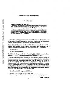
We are now ready to show that the numerical index of a Banach space and the one of its dual do not always coincide. Example 2.3.1 ([13, Example 3.1]). Let us consider the Banach space X = (x, y, z) ∈ c ⊕∞ c ⊕∞ c : lim x + lim y + lim z = 0 . Then, n(X) = 1 and n(X ∗ ) < 1. Proof. We observe that X ∗ = c∗ ⊕1 c∗ ⊕1 c∗ /h(lim, lim, lim)i

so that, writing Z = `31 /h(1, 1, 1)i, we can identify X ∗ ≡ `1 ⊕1 `1 ⊕1 `1 ⊕1 Z

and

X ∗∗ ≡ `∞ ⊕∞ `∞ ⊕∞ `∞ ⊕∞ Z ∗ .

Figure 2.1: The unit ball of Z

With this in mind, we write A to denote the set {(e∗n , 0, 0, 0) : n ∈ N} ∪ {(0, e∗n , 0, 0) : n ∈ N} ∪ {(0, 0, e∗n , 0) : n ∈ N}.

(2.3)

30


Then A is clearly a norming subset of SX ∗ and x∗∗ ∈ ext(BX ∗∗ ), a∗ ∈ A .

|x∗∗ (a∗ )| = 1

(2.4)

Let us prove that n(X) = 1. Indeed, we fix T ∈ L(X) and ε > 0. Since T ∗ is w∗ -continuous and A is norming, we may find a∗ ∈ A such that kT ∗ (a∗ )k > kT k − ε. Now, we take x∗∗ ∈ ext(BX ∗∗ ) such that |x∗∗ (T ∗ (a∗ ))| = kT ∗ (a∗ )k. Since |x∗∗ (a∗ )| = 1 thanks to (2.4), we get v(T ) = v(T ∗ ) > |x∗∗ (T ∗ (a∗ ))| > kT k − ε. It clearly follows that v(T ) = kT k and n(X) = 1.

To show that n(X ∗ ) < 1, we use (2.3) and Proposition 2.2.10 to get n(X ∗ ) 6 n(Z),

and the fact that n(Z) < 1 follows easily from a result due to C. McGregor [89, Theorem 3.1]. Actually, in the real case, the unit ball of Z is an hexagon (see Figure 2.1 above), which is isometrically isomorphic to the space X3 of Proposition 2.2.15, so n(Z) = 1/2. The above example can be pushed forward, to produce even more striking counterexamples. Examples 2.3.2 ([13, Examples 3.3]). (a) There exists a real Banach space X such that n(X) = 1 and n(X ∗ ) = 0. (b) There exists a complex Banach space X satisfying that n(X) = 1 and n(X ∗ ) = 1/e. On the other hand, the fact that the numerical index of the spaces in all the examples above is equal to 1 has nothing to do with the possibility of getting an strict inequality in 2.2. Example 2.3.3. (a) For every t ∈]0, 1] there is a real Banach space Xt with n(Xt ) = t and n(Xt∗ ) = 0. (b) For every t ∈] 1e , 1] there is a complex Banach space Xt with n(Xt ) = t and n(Xt∗ ) = 1e . Let us observe that it is possible to construct more counterexamples by using the spaces CE (KkL) given in section 1.4. As shown in Theorem 2.2.6, if A or A∗ is a C ∗ -algebra, then n(A) = n(A∗ ). The next example shows that it is not possible to go further.

2.3. Numerical index and duality

31

Example 2.3.4 ([78, Example 4.3]). Let us consider the space X = CK(`2 ) ([0, 1]k∆). Then, n(X) = 1 and X ∗ ≡ K(`2 )∗ ⊕1 C0 (Kk∆)∗

and

X ∗∗ ≡ L(`2 ) ⊕1 C0 (Kk∆)∗∗ .

Therefore, X ∗∗ is a C ∗ -algebra, but n(X ∗ ) = 1/2 < n(X). We now present some more results concerning numerical index and duality. The first result is a sufficient condition to get the equality of the numerical index of a Banach space and its dual. We recall that a Banach space X is said to be L-embedded if X ∗∗ = X ⊕1 Xs for some closed subspace Xs of X ∗∗ . We refer to [43] for background. Examples of L-embedded spaces are the reflexive ones (trivial), preduals of von Neumann algebras (in particular, L1 (µ) spaces), the Lorentz spaces d(w, 1) and Lp,1 (see [43, Examples III.1.4 and IV.1.1]). Theorem 2.3.5 ([80, Theorem 2.1]). Let X be an L-embedded space. Then, n(X) = n(X ∗ ). Let us comment that it has been shown recently that separable L-embedded Banach spaces are unique predual of their duals [95]. By a predual of a Banach space Y we mean a Banach space X such that X ∗ is (isometrically isomorphic to) Y . Therefore, it makes sense to ask whether a Banach space X having a unique predual X∗ satisfies n(X∗ ) = n(X). Problem 2.3.6. Let Y be a dual space admitting a unique predual X (up to isometric isomorphisms). Is it true that n(Y ) = n(X)? We recall that a Banach space X is M -embedded if X ⊥ is an L-summand of X ∗∗∗ or, equivalently, if the natural (Dixmier) projection from X ∗∗∗ onto X ∗ is an L-projection (i.e. X ∗∗∗ = iX ∗ (X ∗ ) ⊕1 X ⊥ ). We refer the reader to [43] for more information and background. Typical examples of M -embedded spaces are c0 (Γ) for any set Γ and K(H), the space of compact operators on a Hilbert space H [43, Examples III.1.4]. The following is another particular case in which the equality in (2.2) holds. Theorem 2.3.7 ([80, Theorem 3.3]). Let X be an M -embedded space with n(X) = 1. If Y is a closed subspace of X ∗∗ containing (the canonical copy of) X, then n(Y ) = 1. In particular, n(X ∗ ) = 1 and n(X ∗∗ ) = 1. Remark 2.3.8. It is not always possible to get n(Y ∗ ) = 1 in the above theorem. Indeed, let X be the space given Example 2.3.1. Then, one clearly has that c0 (N × N × N) ⊂ X ⊂ `∞ (N × N × N), c0 (N × N × N) is M -embedded, but n(X ∗ ) < 1.

32


Once we know that the numerical index of a Banach space and the one of its dual may be different, the question arises if two preduals of a given Banach space have the same numerical index. The answer is again negative, as the following result shows. Example 2.3.9 ([13, Example 3.6]). Let us consider the Banach spaces X1 = (x, y, z) ∈ c ⊕∞ c ⊕∞ c : lim x + lim y + lim z = 0

and

X2 = (x, y, z) ∈ c ⊕∞ c ⊕∞ c : x(1) + y(1) + z(1) = 0 .

Then, X1∗ and X2∗ are isometrically isomorphic, but n(X1 ) = 1 and n(X2 ) < 1. The following question might also be addressed. Problem 2.3.10. Let Y be a dual space. Does there exist a predual X of Y such that n(X) = n(Y )? Another interesting issue could be to find isomorphic properties of a Banach space X ensuring that n(X ∗ ) = n(X). On the one hand, Example 2.3.1 shows that Asplundness is not such a property. On the other hand, it is shown in [13, Proposition 4.1] that if a Banach space X with the Radon-Nikodým property has numerical index 1, then X ∗ has numerical index 1 as well. Therefore, the following question naturally arises. Problem 2.3.11. Let X be a Banach space with the Radon-Nikodým property. Is it true that n(X) = n(X ∗ )?

2.4

Banach spaces with numerical index one

The guiding open question on these spaces is the following. Problem 2.4.1. Find necessary and sufficient conditions for a Banach space to have numerical index 1 which do not involve operators. In 1971, C. McGregor [89, Theorem 3.1] gave such a characterization in the finite dimensional case. More concretely, a finite-dimensional normed space X has numerical index 1 if and only if (2.5) |x∗ (x)| = 1 for every x ∈ ext(BX ) and every x∗ ∈ ext(BX ∗ ). It is not clear how to extend this result to arbitrary Banach spaces. If we use literally (2.5) in the infinite-dimensional context, we do not get a sufficient condition, since the set

2.4. Banach spaces with numerical index one

33

ext(BX ) may be empty and this does not imply numerical index 1 (e.g. ext(Bc0 (`2 ) ) = ∅ but n(c0 (`2 )) < 1). On the other hand, (2.5) is not necessary condition. Example 2.4.2 ([53, Examples 5.1 and 5.2]). There is a Banach space X with n(X) = 1 and there are f0 ∈ ext(BX ) and x∗0 ∈ ext(BX ∗ ) satisfying x∗0 (f0 ) = 0. Our first aim in this section is to discuss several reformulations of assertion (2.5) to get either sufficient or necessary conditions for a Banach space to have numerical index 1. Aiming at sufficient conditions, it is not difficult to show that (2.5) implies numerical index 1 for a Banach space X as soon as the set ext(BX ) is large enough to determine the norm of operators on X, i.e. BX = co(ext(BX )). Actually, we may replace ext(BX ) with any subset of SX satisfying the same property. On the other hand, we may replace ext(BX ) by ext(BX ∗∗ ) and the role of ext(BX ∗ ) can be played by any norming subset of SX ∗ . Let us comment that this is is what we did in the proof of Example 2.3.1. We summarize all these ideas in the following proposition. Proposition 2.4.3. Let X be a Banach space. Then, any of the following three conditions is sufficient to ensure that n(X) = 1. (a) There exists a subset C of SX such that co(C) = BX and |x∗ (c)| = 1 for every x∗ ∈ ext(BX ∗ ) and every c ∈ C. (b) |x∗∗ (x∗ )| = 1 for every x∗∗ ∈ ext(BX ∗∗ ) and every x∗ ∈ ext(BX ∗ ). (c) There exists a norming subset A of SX ∗ such that |x∗∗ (a∗ )| = 1 for every x∗∗ ∈ ext(BX ∗∗ ) and every a∗ ∈ A. Let us comment on the converse of the above result. First, condition (a) is not necessary as shown by c0 . Second, it was proved in [13, Example 3.4] that condition (b) is not necessary either, the counterexample being the space given in Example 2.3.1. Finally, a Banach with numerical index 1 in which condition (c) is not satisfied has been discovered very recently [54] (see section 3.4 for details). Necessary conditions in the spirit of McGregor’s result were given in 1999 by G. López, M. Martín, and R. Payá [73]. The key idea was considering denting points instead of general extreme points. Recall that x0 ∈ BX is said to be a denting point of BX if it belongs to slices of BX with arbitrarily small diameter. If X is a dual space and the slices can be taken to be defined by weak∗ -continuous functionals, then we say that x0 is a weak∗ -denting point.

34


Proposition 2.4.4 ([73, Lemma 1]). Let X be a Banach space with numerical index 1. Then, (a) |x∗ (x)| = 1 for every x∗ ∈ ext(BX ∗ ) and every denting point x ∈ BX . (b) |x∗∗ (x∗ )| = 1 for every x∗∗ ∈ ext(BX ∗∗ ) and every weak∗ -denting point x∗ ∈ BX ∗ . This result will play a key role in the next section. Let us comment that, like McGregor original result, the conditions in Proposition 2.4.4 are not sufficient in the infinite-dimensional context. Indeed, the space X = C([0, 1], `2 ) does not have numerical index 1, while BX has no denting points and there are no w∗ -denting points in BX ∗ . Actually, all the slices of BX and the w∗ -slices of BX ∗ have diameter 2 (see [59, Lemma 2.2 and Example on p. 858], for instance). Anyhow, if we have a Banach space X such that BX has enough denting points (if X has the Radon-Nikodým property, for instance), then item (a) in the above proposition combines with Proposition 2.4.3 to characterize the numerical index 1 for X. The same is true for item (b) when BX ∗ has enough weak∗ -denting points (if X is an Asplund space, for instance). Corollary 2.4.5 ([77, Theorem 1] and [79, §1]). Let X be a Banach space. (a) If X has the Radon-Nikodým property, then the following are equivalent: (i) X has numerical index 1. (ii) |x∗ (x)| = 1 for every x∗ ∈ ext(BX ∗ ) and every denting point x of BX .

(iii) |x∗∗ (x∗ )| = 1 for every x∗∗ ∈ ext(BX ∗∗ ) and every x∗ ∈ ext(BX ∗ ). (b) If X is an Asplund space, then the following are equivalent: (i) X has numerical index 1.

(ii) |x∗∗ (x∗ )| = 1 for every x∗∗ ∈ ext(BX ∗∗ ) and every weak∗ -denting point x∗ ∈ BX ∗ . Next chapter is devoted to study a sufficient condition for a Banach space to have numerical index 1, namely the so-called lushness property.

2.5

Renorming and numerical index

In 2003, C. Finet, M. Martín, and R. Payá [30] studied the numerical index from the isomorphic point of view, i.e. they investigated the set N (X) of those values of the numerical index which can be obtained by equivalent renormings of a Banach space X. This study has a precedent in the 1974 paper [108] by K. Tillekeratne, where it is proved that every complex space of dimension greater than one can be renormed to achieve the minimum value of the numerical index; the same is true for real spaces.

2.5. Renorming and numerical index

35

Proposition 2.5.1 ([30, Proposition 1] and [108, Theorem 3.1]). Let X be a Banach space of dimension greater than one. Then 0 ∈ N (X) in the real case, e−1 ∈ N (X) in the complex case. One of the main aims of [30] is to show that N (X) is a interval for every Banach space X. To get this result, the authors use the continuity of the mapping carrying every equivalent norm on X to its numerical index with respect to a metric taken from [8, §18]. Proposition 2.5.2 ([30, Proposition 2]). N (X) is an interval for every Banach space X. As an immediate consequence of the above two results, we get the following. Corollary 2.5.3 ([30, Corollary 3]). If 1 ∈ N (X) for a Banach space X of dimension greater than one, then N (X) = [0, 1] in the real case and N (X) = [e−1 , 1] in the complex case. Since n(`m ∞ ) = 1 for every m, the following particular case arises. Corollary 2.5.4 ([108, Theorem 3.2]). Let m be an integer larger than 1. Then N (Rm ) = [0, 1]

and

N (Cm ) = [e−1 , 1].

Now, one may ask if the above result is also true in the infinite-dimensional context, equivalently, whether or not every Banach space can be equivalently renormed to have numerical index 1. The answer is negative, as shown in the already cited paper [73]. Theorem 2.5.5 ([73, Theorem 3]). Let X be an infinite-dimensional real Banach space with 1 ∈ N (X). If X has the Radon-Nikodým property, then X contains `1 . If X is an Asplund space, then X ∗ contains `1 . It follows that infinite-dimensional real reflexive spaces cannot be renormed to have numerical index 1. But even more is true. Corollary 2.5.6 ([73, Corollary 5]). Let X be an infinite-dimensional real Banach space. If X ∗∗ /X is separable, then 1 ∈ / N (X). It is easy to explain how Theorem 2.5.5 was proved in [73]. Namely, the authors used Proposition 2.4.4, the well-known facts that the unit ball of a space with the Radon-Nikodým property has many denting points and that the dual unit ball of an Asplund space has many weak∗ -denting points (see [11], for instance), and the following sufficient condition for a real Banach space to contain either c0 or `1 .

36


Lemma 2.5.7 ([73, Proposition 2]). Let X be a real Banach space, and assume that there is an infinite set A ⊂ SX such that |x∗ (a)| = 1 for every a ∈ A and every x∗ ∈ ext(BX ∗ ). Then X contains c0 or `1 . Thus, the first open question in this line is the following. Problem 2.5.8. Characterize those Banach spaces which can be equivalently renormed to have numerical index 1. The better result we have in this line is the following, for which we will give a detailed proof in section 6.2. Theorem 2.5.9 ([5, Corollary 4.10]). Let X be an infinite-dimensional real Banach space satisfying that 1 ∈ N (X). Then, X ∗ ⊇ `1 . One may wonder whether the above necessary condition for a Banach space to be renormed with numerical index 1 is also sufficient. The answer is not, as the following example shows. Example 2.5.10 ([12, Example 3.8]). There is a Banach space Y such that Y ∗ is isomorphic to `1 but Y does not admit any equivalent norm with numerical index 1. Indeed, let us consider the real space Y given in [10] such that Y ∗ is isomorphic to `1 and Y has the Radon-Nikodým property. Then, Y is an infinite-dimensional real Banach space having the Radon-Nikodým property and it is also Asplund, so Theorem 2.5.5 shows that it does not admit an equivalent norm with numerical index 1. We propose to study separately necessary and sufficient conditions for a Banach space to be renormable with numerical index 1. With respect to necessary conditions, we have obtained two in the real case, namely Theorems 2.5.5 and 2.5.9. It is not known if they are valid in the complex case; actually, the following especial case remains open. Problem 2.5.11. Does there exist an infinite-dimensional complex reflexive space which can be renormed to have numerical index 1? For more necessary conditions, we suggest to study the following question. Problem 2.5.12. Let X be an infinite-dimensional (real) Banach space satisfying that 1 ∈ N (X). Does X contain c0 or `1 ? With respect to sufficient conditions, the only we know is the following one. We will give

2.5. Renorming and numerical index

37

a detailed proof of it in section 6.2. Theorem 2.5.13 ([12, Corollary 3.6]). Every separable Banach space containing an isomorphic copy of c0 can be equivalently renormed to have numerical index 1. Corollary 2.5.14. Every closed subspace of c0 can be equivalently renormed to have numerical index 1. More possible sufficient conditions are the following. Problem 2.5.15. Let X be a Banach space containing an infinite-dimensional subspace Y such that 1 ∈ N (Y ). Is it true that 1 ∈ N (X)? One may consider an especial case. Problem 2.5.16. Let X be a Banach space containing a subspace isomorphic to `1 . Is it true that 1 ∈ N (X)? We finish this section by showing that the value 1 of the numerical index is very particular. Indeed, it is proved in [30] that “most” Banach spaces can be renormed to achieve any possible value for the numerical index except eventually 1. Recall that a system {(xλ , x∗λ )}λ∈Λ ⊂ X × X ∗ is said to be biorthogonal if x∗λ (xµ ) = δλ,µ for λ, µ ∈ Λ, and long if the cardinality of Λ coincides with the density character of X. Theorem 2.5.17 ([30, Theorem 10]). Let X be a Banach space admitting a long biorthogonal system. Then sup N (X) = 1. Therefore, when the dimension of X is greater than one, N (X) ⊃ [0, 1[ in the real case and N (X) ⊃ [e−1 , 1[ in the complex case. Typical examples of Banach spaces admitting a long biorthogonal system are WCG spaces (see [16]). For instance, if X ∗∗ /X is separable, then the Banach space X is WCG (see [111, Theorem 3], for example) while, in the real case, 1 ∈ / N (X) unless X is finite-dimensional (see Corollary 2.5.6). Therefore, in many cases one of the inclusions of Theorem 2.5.17 becomes an equality. Corollary 2.5.18 ([30, Corollary 11]). Let X be an infinite-dimensional real Banach space such that X ∗∗ /X is separable. Then N (X) = [0, 1[. Let us comment that Theorem 2.5.17 is proved by using a geometrical property that was introduced by J. Lindenstrauss in the study of norn-attaining operators [69] and called

38


property α by W. Schachermayer [104]. It is known that, under the continuum hypothesis, there are Banach spaces which cannot be renormed with property α [38, 90]. Nevertheless, B. Godun and S. Troyanski proved in [38, Theorem 1] that this renorming is possible for Banach spaces admitting a long biorthogonal system; as far as we know, this is the largest class of spaces for which renorming with property α is possible. The question arises if the assumption of having a long biorthogonal system in Theorem 2.5.17 can be dropped. Problem 2.5.19. Is is true that sup N (X) = 1 for every Banach space X? It is also studied in [30] the relationship between the numerical index and the so-called property β [69, 104]. Contrary to property α, property β is isomorphically trivial (J. Partington [92]), but it does not produce such a good result as Theorem 2.5.17. At least, it can be used to prove that N (X) does not reduces to a point when the dimension of X is greater than one. Theorem 2.5.20 ([30, Theorem 9]). Let X be a Banach space with dim(X) > 1. Then N (X) ⊃ [0, 1/3[ in the real case and N (X) ⊃ [e−1 , 1/2[ in the complex case.

2.6

Asymptotic behavior of the set of finite-dimensional spaces with numerical index one

Our aim in this section is to consider the asymptotic behavior (as the dimension grows to infinity) of some parameters related to the Banach-Mazur distance for the family of finitedimensional real normed spaces with numerical index 1. Let us write Nm for the space of all m-dimensional normed spaces endowed with the Banach-Mazur distance d(X, Y ) = inf{kT k kT −1 k : T : X −→ Y isomorphism}

(X, Y ∈ Nm ),

and let us write Mm for the subset consisting of those m-dimensional spaces with numerical index 1. Our aim is to study some questions related to these two spaces. As far as we know, the first result of this kind was given very recently by T. Oikhberg [91]. Theorem 2.6.1 ([91, Theorem 4.1]). There exists a universal positive constant c such that 1

4 d(X, `m 2 ) > cm

for every m > 1 and every X ∈ Mm . √ m m m It is well-known that d(`m m for every m > 1 (see [36, pp. 720] for 1 , `2 ) = d(`∞ , `2 ) = instance). Therefore, the following question arises naturally.

2.7. Relationship to the Daugavet property.

39

Problem 2.6.2. Does there exist a universal constant c > 0 such that √ d(X, `m 2 )>c m for every m > 1 and every X ∈ Mm ? It was observed in [91, pp. 622] that the answer to this question is positive for some class of Banach spaces with numerical index 1: those constructed starting from the real line and producing successively `∞ and/or `1 sums. But not every element of Mm is of this form. Finally, we would like to propose some related questions. Problem 2.6.3. What is the diameter of Mm ? Is it (asymptotically) close to the diameter of Nm ? Problem 2.6.4. What is the biggest possible distance from an element of Nm to the set Mm ?

2.7

Relationship to the Daugavet property.

In every Banach space with the Radon-Nikodým property (in particular in every reflexive space) the unit ball must have denting points. There are Banach spaces X (as C[0, 1], L1 [0, 1], and many others) with an extremely opposite property: for every x ∈ SX and for arbitrarily small ε > 0, the closure of co BX \ (x + (2 − ε)BX ) equals to the whole BX (see Figure 2.2 below). This geometric property of the space is equivalent to the following exotic property of operators on X: for every compact operator T : X −→ X, the so-called Daugavet equation kId + T k = 1 + kT k

(DE)

holds. This property of C[0, 1] was discovered by I. K. Daugavet in 1963 and is called the Daugavet property [58, 59]. Over the years, the validity of the Daugavet equation was proved for some classes of operators on various spaces, including weakly compact operators on C(K) and L1 (µ) provided that K is perfect and µ does not have any atoms (see [112] for an elementary approach), and on certain function algebras such as the disk algebra A(D) or the algebra of bounded analytic functions H ∞ [113, 115]. In the nineties, new ideas were infused into this field and the geometry of Banach spaces having the Daugavet property was studied; we cite the papers of V. Kadets, R. Shvidkoy, G. Sirotkin, and D. Werner [59] and R. Shvidkoy [107] as representatives. Let us comment that the original definition of Daugavet property given in [58, 59] only required rank-one operators to satisfy (DE) and, in such a case, this equation also holds for every bounded operator which does not fix a copy of `1 [107].

40


x

BX \ x + (2 − ε)BX

Figure 2.2: The space `2∞ does not have the Daugavet property

Although the Daugavet property is of isometric nature, it induces various isomorphic restrictions. For instance, a Banach space with the Daugavet property contains `1 [59], it does not have unconditional basis (V. Kadets [50]) and, moreover, it does not isomorphically embed into an unconditional sum of Banach spaces without a copy of `1 [107]. It is worthwhile to remark that the latest result continues a line of generalization ([49], [57], [59]) of the well known theorem by A. Pełczyński [94] that L1 [0, 1] (and so C[0, 1]) does not embed into a space with unconditional basis. The state-of-the-art on the Daugavet property can be found in [114]. Let us explain the relation between (DE) and the numerical range of an operator. The following result appeared for the first time in the aforementioned paper [21] by J. Duncan, C. McGregor, J. Pryce, and A. White. Lemma 2.7.1. Let X be a Banach space and T ∈ L(X). Then, T satisfies (DE) if and only if sup Re V (T ) = kT k. Therefore, X has the Daugavet property if and only if all rank-one operators T ∈ L(X) satisfy sup Re V (T ) = kT k. Let us introduce a needed definition. An operator T on a Banach space X satisfies the alternative Daugavet equation if the norm equality max kId + ω T k = 1 + kT k ω∈T

(aDE)

holds. A Banach space X is said to have the alternative Daugavet property if every rank-one

2.7. Relationship to the Daugavet property.

41

operator on X satisfies (aDE). In such a case, every weakly compact operator on X also satisfies (aDE) [85, Theorem 2.2]. Therefore, X has the alternative Daugavet property if and only if v(T ) = kT k for every weakly compact operator T ∈ L(X). It follows from the above lemma that Lemma 2.7.2. Let X be a Banach space and T ∈ L(X). Then, T satisfies (aDE) if and only if v(T ) = kT k. Therefore, X has the alternative Daugavet property if and only if all rank-one operators T ∈ L(X) satisfy v(T ) = kT k. Therefore, it was known since 1970 that every bounded linear operator on C(K) or L1 (µ) satisfies (aDE), a fact that was rediscovered and reproved in some papers from the eighties and nineties as the ones by Y. Abramovich [1], J. Holub [46], and K. Schmidt [105]. Let us comment that, contrary to the Daugavet property, the alternative Daugavet property depends upon the base field (e.g. C has it as a complex space but not as a real space). For more information on the alternative Daugavet property we refer to the papers [79, 85]. From the second one we take the following geometric characterizations of the alternative Daugavet property. Proposition 2.7.3 ([85, Propositions 2.1 and 2.6]). Let X be a Banach space. Then, the following are equivalent. (i) X has the alternative Daugavet property. (ii) For all x0 ∈ SX , x∗0 ∈ SX ∗ and ε > 0, there is some x ∈ SX such that |x∗0 (x)| > 1 − ε

and

kx + x0 k > 2 − ε.

(ii∗ ) For all x0 ∈ SX , x∗0 ∈ SX ∗ and ε > 0, there is some x∗ ∈ SX ∗ such that |x∗ (x0 )| > 1 − ε

and

kx∗ + x∗0 k > 2 − ε.

(iii) BX = co T BX \ x + (2 − ε)BX for every x ∈ SX and every ε > 0 (see Figure 2.3 below). ∗ (iii∗ ) BX ∗ = cow T BX ∗ \ x∗ + (2 − ε)BX ∗ for every x∗ ∈ SX ∗ and every ε > 0. (iv) BX ∗ ⊕∞ X ∗∗ = cow

∗

{(x∗ , x∗∗ ) : x∗ ∈ ext(BX ∗ ), x∗∗ ∈ ext(BX ∗∗ ), |x∗∗ (x∗ )| = 1} .

It is clear that both spaces with the Daugavet property and spaces with numerical index 1 have the alternative Daugavet property. Both converses are false: the space c0 ⊕1 C([0, 1], `2 ) has the alternative Daugavet property but fails the Daugavet property and its numerical index is not 1 [85, Example 3.2]. Nevertheless, under certain isomorphic conditions, the alternative Daugavet property forces the numerical index to be 1.

42


x BX \ (−x + (2 − ε)BX )

BX \ (x + (2 − ε)BX )

Figure 2.3: The space `2∞ has the alternative Daugavet property

Proposition 2.7.4 ([73, Remark 6]). Let X be a Banach space with the alternative Daugavet property. If X has the Radon-Nikodým property or X is an Asplund space, then n(X) = 1. With this result in mind, one realizes that the necessary conditions for a real Banach space to be renormed with numerical index 1 given in section 2.5 (namely Theorem 2.5.5 and Corollary 2.5.6), can be written in terms of the alternative Daugavet property. Even more, in the proof of Proposition 2.4.4 given in [73], only rank-one operators are used and, therefore, it can be also written in terms of the alternative Daugavet property. Proposition 2.7.5 ([73, Lemma 1 and Remark 6]). Let X be a Banach space with the alternative Daugavet property. Then, (a) |x∗∗ (x∗ )| = 1 for every x∗∗ ∈ ext(BX ∗∗ ) and every weak∗ -denting point x∗ ∈ BX ∗ . (b) |x∗ (x)| = 1 for every x∗ ∈ ext(BX ∗ ) and every denting point x ∈ BX . Proposition 2.7.6 ([85, Remark 2.8]). Let X be an infinite-dimensional real Banach space with the alternative Daugavet property. If X has the Radon-Nikodým property, then X contains `1 . If X is an Asplund space, then X ∗ contains `1 . In particular, X ∗∗ /X is not separable.

The above two results give us an indication of why it is difficult to find characterizations

2.8. Smoothness, convexity and numerical index 1

43

of Banach spaces with numerical index 1 that do not involve operators. Indeed, it is not easy to construct noncompact operators on an abstract Banach space. Thus, when one uses the assumption that a Banach space has numerical index 1, only the alternative Daugavet property can be easily exploited. Of course, things are easier if one is working in a context where the alternative Daugavet property ensures numerical index 1, as it happens with Asplund spaces and spaces with the Radon-Nikodým property. We will study a more general isomorphic property for which the alternative Daugavet property and the numerical index 1 are equivalent in chapter 4. In particular, the following important result will be shown. Theorem 2.7.7. Let X be a Banach space which does not contain any copy of `1 and having the alternative Daugavet property. Then, n(X) = 1. On the other hand, it is not possible to find isomorphic properties ensuring that the alternative Daugavet property and the Daugavet property are equivalent. Proposition 2.7.8 ([85, Corollary 3.3]). Let X be a Banach space with the alternative Daugavet property. Then there exists a Banach space Y , isomorphic to X, which has the alternative Daugavet property but fails the Daugavet property.

We may then look for isometric conditions that allow passing from the alternative Daugavet property to the Daugavet property. Having a complex structure could be such a condition. Problem 2.7.9. Let X be a complex Banach space such that XR has the alternative Daugavet property. Does it follow that X (equivalently XR ) has the Daugavet property?

2.8

Smoothness and convexity for Banach spaces with numerical index 1

We present here some prohibitive isometric conditions for a Banach space to have numerical index 1. Actually, the usage of this hypothesis is done through the alternative Daugavet property. Theorem 2.8.1. Let X be a Banach space with the alternative Daugavet property and dimension greater than one. Then, X ∗ is neither smooth nor strictly convex. Proof. Since the dimension of X is greater than 1, we may find x0 ∈ SX and x∗0 ∈ SX ∗ such that x∗0 (x0 ) = 0. Then, we consider the norm-one operator T = x∗0 ⊗ x0 , which satisfies T 2 = 0. On the other hand, thanks to [3, Theorem 1.2], there is a sequence of norm-one operators (Tn ) converging in norm to T and such that the adjoint of each of them attains its

44


numerical radius. Moreover, we may suppose that all the Tn ’s are compact by [3, Remark 1.3]. Since X has the alternative Daugavet property, we get v(Tn∗ ) = v(Tn ) = kTn k = 1. As the operators Tn∗ attain their numerical radius, for every positive integer n, we may find λn ∈ T and (x∗n , x∗∗ n ) ∈ SX ∗ × SX ∗∗ such that ∗ λn x∗∗ n (xn ) = 1

and

If X ∗ is smooth, we deduce that

∗∗ ∗∗ ∗ ∗ ∗ Tn (xn ) (xn ) = x∗∗ n (Tn (xn )) = 1. n∈N .

∗∗ Tn∗∗ (x∗∗ n ) = λ n xn

Thus,

(2.6)

∗∗ 2 ∗∗ 2 ∗∗ [T ] (x )

n n = kλn xn k = 1

(n ∈ N).

But, since Tn −→ T and T 2 = 0, we have that [Tn∗∗ ]2 −→ 0, a contradiction. If X ∗ is strictly convex, we deduce from (2.6) that Tn∗ (x∗n ) = λn x∗n

n∈N ,

which leads to a contradiction the same way as before.

Corollary 2.8.2. Let X be a Banach space with n(X) = 1. Then, X ∗ is neither smooth nor strictly convex. As a consequence of the above result, we get that n(H 1 ) < 1, where H 1 represents the Hardy space. Actually, we have more. Example 2.8.3. Let X be C(T)/A(D). Then, its dual X ∗ = H 1 is smooth (see [43, Remark IV.1.17], for instance), so X does not have the alternative Daugavet property by Theorem 2.8.1 and neither does X ∗ = H 1 . In particular, n(X) < 1 and n(X ∗ ) < 1. Remarks 2.8.4. (a) The proof of Theorem 2.8.1 can be adapted to yield the following result. Let X be a Banach space with the alternative Daugavet property and such that the set of compact operators attaining its numerical radius is dense in the space of all compact operators. Then, X is neither strictly convex nor smooth, unless it is one-dimensional. Indeed, we may follow the proof of Theorem 2.8.1 (without considering adjoint operators) to get the result.

2.8. Smoothness, convexity and numerical index 1

45

(b) It is known that for Banach spaces with the Radon-Nikodým property, the set of compact operators attaining their numerical radius is dense in the space of all compact operators [3, Theorem 2.4]. Therefore, we get that a Banach space having the Radon-Nikodým property and the alternative Daugavet property is neither smooth nor strictly convex, unless it is one-dimensional. (c) Actually, the above result was essentially known. Namely, if X has the alternative Daugavet property and the Radon-Nikodým property, then X is an almost-CL-space [77, Theorem 1]. It is clear that a (non-trivial) almost-CL-space cannot be strictly convex. On the other hand, the fact that a non-trivial real almost-CL-space cannot be smooth follows from a very recent result [14, Theorem 3.1]. (d) The fact that there are Banach spaces in which the set of numerical radius attaining operators is not dense in the space of all operators was discovered in 1992 [93]. Nevertheless, we do not know of any Banach space for which the set of compact operators which attain their numerical radius is not dense in the space of all compact operators. (e) Let us comment that it is also an open problem whether a Banach space with the Daugavet property can be smooth or strictly convex. We recall that the Daugavet property implies the alternative Daugavet property (and the converse result is not true). Therefore, an example of a smooth or strictly convex Banach space with the Daugavet property would give an example of a Banach space where the rank-one operators cannot be approximated by compact operators attaining the numerical radius.

More prohibitive results for the alternative Daugavet property are the following. A point x in SX is said to be weakly midpoint locally uniformly rotund or WMLUR if for any sequence (yn ) in BX , limn kx ± yn k 6 1 implies limn yn = 0 in the weak topology. Proposition 2.8.5. Let X be a Banach space with the alternative Daugavet property. Then, BX fails to contain a WLUR point, unless X is one-dimensional. The above result is not true if we replace the WLUR point by a point of Fréchet smoothness. For instance, n(c0 ) = 1 but the norm of c0 is Fréchet differentiable at a dense subset of Sc0 since c0 is Asplund. But it is not difficult to show that a Banach space with the alternative Daugavet property cannot have a Fréchet smooth norm, unless it is one-dimensional. Proposition 2.8.6. Let X be a Banach space with the alternative Daugavet property. Then, the norm of X is not Fréchet smooth, unless X is one-dimensional. Let us comment that without completeness, it is possible to find an isometric predual of L1 (µ) which is strictly convex. Example 2.8.7. There is a non-complete isometric predual of an L1 (µ)-space (in particular,

46


it has numerical index 1) which is strictly convex. The completion of the above example (which of course also has numerical index 1) is not strictly convex.

Chapter

3

Lush spaces The classical formula kT k = sup{|hT x, xi| : x ∈ X, kxk = 1} for the norm of a self-adjoint operator T on a Hilbert space X can be rewritten, thanks to the well-known representation of the dual, as kT k = sup{|x∗ (T x)| : x ∈ X, x∗ ∈ X ∗ , x∗ (x) = kx∗ k = kxk = 1}.

(3.1)

For a non self-adjoint operator this formula may fail. Nevertheless, there are some Banach spaces X in which equality (3.1) is valid for every bounded linear operator T on X. As the reader may imagine, this are the Banach spaces with numerical index 1. Among these spaces are all classical C(K) and L1 (µ) spaces. A big difficulty when studying Banach spaces with numerical index 1 is that this property deals with all operators on the space and we do not know of any characterization of it in terms of the space and its successive duals. The previous solutions to this difficulty have been to deal with either weaker or stronger geometrical properties. Let us briefly give an account of some of them. Let X be a real or complex Banach space. (a) X is said to be a CL-space if BX is the absolutely convex hull of every maximal convex subset of SX . (b) We say that X is an almost-CL-space if BX is the closed absolutely convex hull of every maximal convex subset of SX . (c) X is lush if for every x, y ∈ SX and every ε > 0, there is a slice S = S(BX , x∗ , ε) with x∗ ∈ SX ∗ such that x ∈ S and dist (y, aconv(S)) < ε. (d) X has numerical index 1 (n(X) = 1 in short) if v(T ) = kT k for every T ∈ L(X). (e) We say that X has the alternative Daugavet property provided that every rank-one operator T ∈ L(X) satisfies v(T ) = kT k. The same equality is then satisfied by all weakly compact operators on X [85, Theorem 2.2]. 47

48

Chapter 3. Lush spaces

The implications (a) =⇒ (b) =⇒ (c) and (d) =⇒ (e) are clear and none of them reverses (see [13, §3 and §7] for a detailed account). Also, (c) =⇒ (d) by [13, Proposition 2.2] and it has been very recently shown that this implication does not reverses [54]. Some additional comments on the above properties may be in place. CL-spaces where introduced in 1960 by R. Fullerton [35] and it was later shown that a finite-dimensional Banach space has numerical index 1 if and only if it is a CL-space ([89, Theorem 3.1] and [72, Corollary 3.7]). Therefore, the above five properties are equivalent in the finite-dimensional case. All C(K) spaces as well as real L1 (µ) spaces are CL-spaces, while infinite-dimensional complex L1 (µ) spaces are only almost-CL-spaces (see [87]). Almost-CL-spaces first appeared without a name in the memoir by J. Lindenstrauss [68] and were further discussed by Å. Lima [71, 72] who showed that real Lindenstrauss spaces (i.e. isometric preduals of L1 (µ)) are CL-spaces [71, §3] and complex Lindenstrauss spaces are almost-CL-spaces [72, §3]. The disk algebra is another classical example of an almost-CL-space [8, Theorem 32.9]. More information can be found in [14, 77, 87, 97]. The concept of lushness was introduced recently in [13] as a geometrical property of a Banach space which ensures that the space has numerical index 1. The concept of lushness is proven to be a useful tool in the theory of numerical index of Banach spaces since in [13] it helped to construct an example showing that numerical index is not inherited in general by the dual space, a latent question in the theory from the beginning of the subject. Also, in [63] the lushness was applied for estimating the related concept of polynomial numerical index in some real spaces like c0 or `1 .

3.1

Examples of lush spaces

The following observation is immediate. Remark 3.1.1. Any almost-CL-space is lush.

The name of CL-space comes from the fact that this property is shared by the real spaces C(K) and L1 (µ) [71]. In the complex case, C(K) is a CL-space while L1 (µ) is an almost-CLspace [87]. This gives us the first examples of lush spaces. Example 3.1.2. The real or complex spaces C(K) and L1 (µ) are lush. The converse of Remark 3.1.1 is not true in general (see [13, Example 3.4]), but this is the case for Banach spaces having the Radon-Nikodým property. Proposition 3.1.3. Let X be a Banach space with the Radon-Nikodým property. Then, the following are equivalent:

3.1. Examples of lush spaces

49

(i) X has numerical index 1, (ii) There are a compact Hausdorff space K and a linear isometry J : X → C(K) such that |x∗∗ (J ∗ δs )| = 1 for all s ∈ K and x∗∗ ∈ ext(BX ∗∗ ), (iii) |x∗∗ (x∗ )| = 1 for all x∗ ∈ ext(BX ∗ ) and x∗∗ ∈ ext(BX ∗∗ ), (iv) X is an almost-CL-space, (v) X is lush. In the finite-dimensional setting, Proposition 3.1.3 has an even better shape. Proposition 3.1.4. Let X be a finite-dimensional Banach space. Then, the following are equivalent: (i) (ii) (iii) (iv)

X has numerical index 1, |x∗ (x)| = 1 for every x∗ ∈ ext(BX ∗ ) and every x ∈ ext(BX ), X is a CL-space, X is lush.

For Asplund spaces we also have a characterization of lushness. Some notation is needed. Given a completely regular Hausdorff topological space Ω, we write Cb (Ω) to denote the Banach space of all K-valued bounded continuous functions on Ω, endowed with the supremum norm. Theorem 3.1.5. Let X be an Asplund space. Then, the following are equivalent: (i) n(X) = 1, (ii) There is a completely regular Hausdorff topological space Ω and an isometric embedding J : X −→ Cb (Ω) such that |x∗∗ (J ∗ (δs ))| = 1 for every s ∈ Ω and x∗∗ ∈ ext(BX ∗∗ ), (iii) There is a subset A ⊂ BX ∗ norming for X such that |x∗∗ (a∗ )| = 1 for every a∗ ∈ A and every x∗∗ ∈ ext(BX ∗∗ ), (iv) For each x ∈ SX and ε > 0 there exists x∗ ∈ SX ∗ such that x ∈ S = S(BX , x∗ , ε)

and

BX = aconv(S),

(v) X is lush. The equivalences above lead us to consider sufficient conditions for lushness which will be useful. Proposition 3.1.6. Let X be a Banach space. We consider the following assertions. (a) There is a completely regular Hausdorff topological space Ω and an isometric embedding J : X −→ Cb (Ω) such that |x∗∗ (J ∗ (δs ))| = 1 for every s ∈ Ω and x∗∗ ∈ ext(BX ∗∗ ),

(b) There is a norming set A ⊂ BX ∗ for X such that |x∗∗ (a∗ )| = 1 for every a∗ ∈ A and every x∗∗ ∈ ext(BX ∗∗ ),

50


(c) For each x ∈ SX and ε > 0 there exists x∗ ∈ SX ∗ such that x ∈ S = S(BX , x∗ , ε)

and

BX = aconv(S),

(d) X is lush. Then (a) ⇔ (b) ⇒ (c) ⇒ (d). We are giving now two classes of spaces where the above proposition applies. The first R class consists of preduals of L1 (µ) spaces. Indeed, it is clear that ϕf dµ = 1 for every f ∈ ext(BL1 (µ) ) and every ϕ ∈ ext(BL∞ (µ) ). Now, if L1 (µ) has a predual X, then the set ext(BL1 (µ) ) is norming for X and condition (b) of Proposition 3.1.6 applies. Example 3.1.7. The preduals of any L1 (µ) space are lush. Let us comment that, in the real case, preduals of L1 (µ) spaces are actually CL-spaces [71, §3]. The second class of spaces in which Proposition 3.1.6 applies is the one of nicely embedded spaces in Cb (Ω) spaces. Following [113], a Banach space X is said to be nicely embedded in Cb (Ω) if there exists a linear isometry J : X −→ Cb (Ω) such that for all s ∈ Ω the following properties are satisfied: (N1) kJ ∗ δs k = 1. (N2) span(J ∗ δs ) is an L-summand in X ∗ . It is immediate that nicely embedded spaces fulfill condition (a) in Proposition 3.1.6, so they are lush. Example 3.1.8. Any Banach space which nicely embeds into a Cb (Ω) space is lush. An important family of nicely embedded spaces is the one of function algebras [113]. A function algebra A on a compact Hausdorff space K is a closed subalgebra of the space of complex-valued functions C(K) separating the points of K and containing the constant functions. Example 3.1.9. Every function algebra is lush. In particular, the disk algebra and H ∞ are lush.

Another class of lush spaces was introduced in the aforementioned paper [13], the so-called C-rich subspaces of C(K).

3.2. Lush renormings

51

Definition 3.1.10. Let K be a compact Hausdorff space. A closed subspace X of C(K) is said to be C-rich if for every nonempty open subset U of K and every ε > 0, there is a positive function h of norm 1 with support inside U such that the distance from h to X is less than ε. Example 3.1.11 ([13, Theorem 2.4]). C-rich subspaces of C(K) are lush. Some examples and remarks about C-rich subspaces will be useful. Remarks 3.1.12. (a) Due to [13, Proposition 2.5], if K is a perfect compact space, then every finite-codimensional subspace of C(K) is C-rich and, in particular, lush. (b) If one considers `∞ as C(βN), then c0 is C-rich in `∞ . Indeed, this follows easily from the fact that N is a dense subset of βN consisting of isolated points. (c) If X ⊂ C(K) is C-rich, then every subspace Y ⊂ C(K) containing X is C-rich. (d) In particular, every subspace of `∞ containing c0 is C-rich. (e) Let K be an infinite compact set and X be a Banach space such that it is C-rich in C(K). Then, X contains an isomorphic copy of c0 . Indeed, we take a sequence of disjoint open sets Vn ⊂ K. Since X is C-rich in C(K), for ε > 0 and n ∈ N we can find fn ∈ C(K) such that supp(fn ) ⊂ Vn ,

fn > 0,

kfn k = 1,

and dist(fn , X) 6

ε . 2n

The sequence {fn } is a c0 -basic sequence in C(K), and a perturbation argument gives us a basic sequence in X which is equivalent to {fn } and so, it spans an isomorphic copy of c0 .

3.2

Lush renormings

Our goal in this section is to prove that a separable Banach space containing an isomorphic copy of c0 can be equivalently renormed to be lush (in particular, to have numerical index 1). To do so, we need the following result which characterizes isomorphically the separable Banach spaces containing c0 . Theorem 3.2.1. For a separable infinite-dimensional Banach space X, the following conditions are equivalent: (i) X contains an isomorphic copy of c0 , (ii) X is isomorphic to a rich subspace of `∞ = C(βN), (iii) X is isomorphic to a rich subspace of some C(K).

52


The following result is an evident consequence of the above theorem. Corollary 3.2.2. Every separable Banach space containing an isomorphic copy of c0 can be equivalently renormed to be lush.

The following is an interesting particular case. Corollary 3.2.3. Every closed subspace of c0 can be renormed to be lush. The construction can be stretched to get the following result. Theorem 3.2.4. Let X be a separable Banach space containing c0 . Then, there is a Banach space Z isomorphic to X such that n(Z) = 1 and n(Z ∗ ) = 0 in the real case, n(Z ∗ ) = 1/e in the complex case.

3.3

Some reformulations of lushness

The results we are going to present are useful reformulations of lushness. Proposition 3.3.1. Let X be a Banach space and G ⊂ SX ∗ be a norming rounded subset. Then, the following are equivalent: (i) X is lush. (ii)R In the real case: for every x ∈ SX , y ∈ BX and ε > 0, there exist λ1 , λ2 > 0, λ1 + λ2 = 1 and x1 , x2 ∈ BX such that kx + x1 + x2 k > 3 − ε and ky − (λ1 x1 − λ2 x2 )k < ε (ii)C In the complexP case: For every x ∈ SX , y ∈ BX , n ∈ N and ε > 0, there exist λ1 , . . . , λn > 0, nk=1 λk = 1 and x1 , . . . , xn ∈ BX such that

n

x + P xk > n + 1 − ε

k=1

and

n

y − P λk exp

k=1

2πik n

2π xk

0, there is x∗ ∈ G such that x ∈ S = S(BX , x∗ , ε) and dist (y, aconv(S)) < ε.

3.3. Some reformulations of lushness

53

The following is the main application of the above characterization. Corollary 3.3.2. For a Banach space X the following two conditions are equivalent: (i) X is lush, (ii) Every separable subspace E ⊂ X is contained in a separable lush subspace Y such that E ⊂ Y ⊂ X. In the separable case, it is possible to give more characterizations of lushness which will give some important consequences. Theorem 3.3.3. For a separable Banach space X, the following are equivalent: (i) X is lush. ˜ ⊂ ext(BX ∗ ) such that BX = aconv(S(x∗ , ε)) for every (ii) There is a norming subset K ∗ ˜ ε > 0 and for every x ∈ K.

˜ ⊂ ext(BX ∗ ) such that for every x∗ ∈ K ˜ and for every (iii) There is a norming subset K 1 ∗ ∗ ∗ x2 ∈ SX ∗ there is θ ∈ T such that kx1 + θx2 k = 2. We may get two interesting consequences in the real case. Corollary 3.3.4. Let X be a lush real separable space. Then, there is a subset A of SX ∗ norming for X such that for every a∗ ∈ A one has BX = aconv {x ∈ SX : a∗ (x) = 1} .

Corollary 3.3.5. Let X be a real Banach space which is lush. Then, X is neither strictly convex nor smooth, unless it is one-dimensional.

We do not know whether the above two results are true in the complex case. We do not know either whether there are real strictly convex Banach spaces with numerical index 1 others than R. As a consequence of the corollary above, we get a negative answer to a problem by M. Popov. Corollary 3.3.6. A C-rich closed subspace of the real space C[0, 1] is neither strictly convex nor smooth. It is known that a subspace X of C[0, 1] is C-rich whenever C[0, 1]/X does not contain a copy of C[0, 1] (see [56, Proposition 1.2 and Definition 2.1]). Therefore, the following is a

54


particular case of the above proposition. Corollary 3.3.7. Let X be a closed subspace of the real space C[0, 1]. If X is smooth or strictly convex, then C[0, 1]/X contains an isomorphic copy of C[0, 1]. Finally, another interesting consequence of Theorem 3.3.3 is the following. We will improve this result in chapter 4. Corollary 3.3.8. Let X be an infinite-dimensional real lush Banach space. Then X ∗ ⊆ `1 . Let us finish the section with another reformulation of lushness only valid in the real case.

y

z

x + γ1 z

x

x + γ2 z

Figure 3.1: `2∞ is lush

Proposition 3.3.9. Let X be a real Banach space. Then, the following are equivalent: (i) X is lush, (ii) for every x ∈ SX , y ∈ BX and every ε > 0, there are z ∈ SX , γ1 , γ2 ∈ R with |γ1 − γ2 | = 2, such that kx + zk > 2 − ε

and

ky + γi zk 6 1 + ε (i = 1, 2).

See Figure 3.1 for an interpretation of this property in dimension 2. An interesting ap-

3.4. Lushness is not equivalent to numerical index 1

55

plication of the above characterization of lushness if the following characterization of C-rich subspaces of C(K)-spaces for K perfect taken from [54, §6]. Theorem 3.3.10. Let K be a perfect compact space and let Y be a subspace of the real space C(K). Then, Y is C-rich if and only if every subspace Z ⊂ X containing Y is lush.

3.4

Lushness is not equivalent to numerical index 1

We present an example constructed in [54] of a Banach space with numerical index 1 which is not lush. Consider Ω = [0, 2] equipped with the standard Lebesgue measure. Introduce a partition F Ω = ∞ ∆ into subsets of positive measure with ∆0 = [0, 1]. We consider all L∞ (∆n ) n n=0 (in the natural way) as subspaces of L∞ [0, 2]. We denote by F the subspace of L∞ [1, 2], consisting of the functions satisfying the condition Z f dλ = 0 (n ∈ N). ∆n

For a fixed dense countable subset {fm : m ∈ N} ⊂ SL2 [0,1] , let us define an operator J : L∞ [0, 1] −→ L∞ [1, 2] as follows: ! X Z g ∈ L∞ [0, 1] . J(g) = gfm dλ 1∆m m∈N

[0,1]

Observe that for every g ∈ L∞ [0, 1] one has Z kJ(g)k = sup g fm dλ = kgkL2 [0,1] , m∈N [0,1]

so J is a weakly compact operator mapping every modulus-one function from L∞ [0, 1] into a norm-one element of L∞ [1, 2]. Finally, denote Z = g + 2J(g) + f : g ∈ L∞ [0, 1], f ∈ F .

Theorem 3.4.1. Z is a weak∗ -closed C-rich subspace of L∞ [0, 2] such that for Y = ⊥ Z ⊂ L1 [0, 2], the quotient X = L1 [0, 2]/Y is a Banach space which is not lush, but whose dual X ∗ = Z is lush. We now enunciate other properties of the space X constructed in the above theorem. Remarks 3.4.2. Let X be the space constructed in Theorem 3.4.1. (a) X has numerical index 1 but it is not lush.

56


(b) It was asked in [55, Problem 13] and in [13, Remark 3.5], whether for every Banach space E with numerical index one, the subset of SE ∗ given by A(E) = {x∗ ∈ SE ∗ : |x∗∗ (x∗ )| = 1 for every x∗∗ ∈ ext(BE ∗∗ )} is norming for E. Since this condition implies lushness of E [12, Theorem 2.1], we have that A(X ) is not norming and our space X answers in the negative the cited question. (c) Even more, the set A(X ) is empty. The following result gives the unique true implication between the lushness of a space and lushness of the dual or of the bidual. Proposition 3.4.3. Let X be a Banach space. If X ∗∗ is lush, then X is lush.

3.5

Stability results for lushness

We present here some results which can be used to produce more examples of lush spaces. The first two results deal with ultrapoducts and ultrapower. Let us recall the notion of (Banach) ultraproducts [45]. Let U be a free ultrafilter on N, and let {Xn }n∈N be a sequence of Banach spaces. We can consider the `∞ -sum of the family, [⊕n∈N Xn ]`∞ , together with its closed subspace NU =

{xn }n∈N ∈ [⊕n∈N Xn ]`∞ : lim kxn k = 0 . U

The quotient space (Xn )U = [⊕n∈N Xn ]`∞ /NU is called the ultraproduct of the family {Xn }n∈N relative to the ultrafilter U. Let (xn )U stand for the element of (Xn )U containing a given family {xn } ∈ [⊕n∈N Xn ]`∞ . It is easy to check that k(xn )U k = lim kxn k. U

If all the Xn are equal to the same Banach space X, the ultraproduct of the family is called the U-ultrapower of X and it is usually denoted by XU . Proposition 3.5.1. Let {Xn }n∈N be a sequence of lush spaces and let U be a free ultrafilter on N. Then the ultraproduct E = (Xn )U is lush. Proposition 3.5.2. Let X be a Banach space and U be a free ultrafilter on N. Then, the ultrapower E = (X)U is lush if and only if X is lush. Next we would like to deal with absolute sums of Banach spaces. Let us recall that a norm k · ka on Rn is said to be an absolute norm if k(a1 , . . . , an )ka = k(|a1 |, . . . , |an |)ka a1 , . . . , an ∈ R

3.5. Stability results for lushness

57

n and k(1, 0, . . . , 0)ka = · · · = k(0, . . . , 0, 1)ka = 1. If E = (R , k · ka ) is a space with an absolute norm and X1 , . . . , Xn are Banach spaces, we write X = X1 ⊕ X2 ⊕ . . . ⊕ Xn E to denote the E-direct sum (or the E-absolute sum) of X1 , . . . , Xn , that is, X = X1 ⊕ · · · ⊕ Xn endowed with the norm k(x1 , . . . , xn )k = k(kx1 k, . . . , kxn k)ka

For background, we refer the reader to [8, § 21]. Easy examples of absolute norms are the `p -norms for 1 6 p 6 ∞ leading to the `p -direct sums of Banach spaces. Theorem 3.5.3. Let E = (Rn , k · k) be a Banach space with an absolute norm. Then, the following are equivalent. (i) E is lush. (ii) For every collection X1 , X2 , . . . , Xn of lush spaces, the E-direct sum of them is lush. Although the above theorem only deals with finite sums of lush spaces, one can deduce from it the lushness of some infinite sums. Corollary 3.5.4. Let {Xi : i ∈ I} be a family of lush spaces. Then the c0 -, `1 - and `∞ -sums of the family are also lush.

The final results in this section deal with vector valued continuous function spaces. Proposition 3.5.5. Let E be a lush Banach space and K be a Hausdorff compact. Then, the (real or complex) space C(K, E) is also lush. The next result shows that C-rich subspaces are lush also in the vector-valued case. The proof is valid in the real case only. We need to define first C-rich subspaces of C(K, E) spaces. Recall that for α ∈ C(K) and x ∈ E, α ⊗ x ∈ C(K, E) denotes the function t 7−→ α(t)x. Definition 3.5.6. Let K be a compact space and let E be a Banach space. A subspace X of C(K, E) is called C-rich if for every ε > 0, every x ∈ E and every open subset U of K, there exists a nonnegative function α ∈ C(K) with kαk = 1 and supp(α) ⊂ U such that dist(α ⊗ x, X) < ε. Proposition 3.5.7. Let E be a lush real Banach space and K be a Hausdorff compact space. Then, every C-rich subspace X of C(K, E) is also lush.

58


Chapter

4

Slicely countably determined Banach spaces A (separable) Banach space X is slicely countably determined if for every closed convex bounded subset A of X there is a sequence of slices (Sn ) such that each slice of A contains one of the Sn . SCD-spaces form a joint generalization of spaces not containing `1 and those having the Radon-Nikodým property. We present many examples and several properties of this class. We give some applications to Banach spaces with the Daugavet and the alternative Daugavet properties, lush spaces and Banach spaces with numerical index 1. We refer to the manuscript [5] for a detailed account of all the material in this chapter. We recall some facts about the Daugavet property, the alternative Daugavet property and Banach spaces with numerical index 1 which will be useful to understand the motivation of the SCD property. A Banach space X has the Daugavet property if every rank-one operator T ∈ L(X) satisfies kId + T k = 1 + kT k.

(DE)

In this case, all operators on X which do not fix copies of `1 (in particular, weakly compact operators) also satisfy (DE) [107]. If every rank-one operator T ∈ L(X) satisfies the norm equality max kId + θ T k = 1 + kT k (aDE) θ∈T

(T being the set of modulus one scalars), X has the alternative Daugavet property and then all weakly compact operators on X also satisfy (aDE). A Banach space has numerical index 1 if every T ∈ L(X) satisfies (aDE). It follows from the above discussion that

Daugavet property ==⇒ Alternative Daugavet property ⇐== Numerical index 1

None of the above implications reverses in general [85, Example 3.2]. For the first implication, it is even known that it is not reversible under any isomorphic property [85, Corollary 3.3]. On the other hand, it is known that the second implication reverses for Asplund spaces and for Banach spaces with the Radon-Nikodým property [73, Remark 6]. 59

60

Chapter 4. Slicely countably determined Banach spaces

The SCD property is sufficient to get numerical index 1 from the alternative Daugavet property (actually provides lushness) and it is weaker than both RNP and being Asplund (for separable spaces). Actually, this property is satisfied by both separable strongly regular spaces and separable Banach spaces which do not contain copies of `1 . This is our main motivation of the study of SCD spaces.

4.1

Slicely countably determined sets

Given a real or complex Banach space, we write SX for its unit sphere and BX for its closed unit ball. The dual space of X is denoted by X ∗ and L(X) is the Banach algebra of all bounded linear operators from X to itself. A slice of a convex subset A of X is a nonempty subset of the form S(A, x∗ , ε) = {x ∈ A : Re x∗ (x) > sup Re x∗ (A) − ε} and conv(·) stands for the closed convex hull. Definition 4.1.1. Let X be a Banach space and let A be a convex bounded subset of X. The set A is said to be slicely countably determined (SCD set in short) if there is a countable family {Sn : n ∈ N} of slices of A satisfying one of the following equivalent conditions: (i) every slice of A contains one of the Sn , (ii) A ⊆ conv(B) for every B ⊆ A intersecting all the sets Sn ,

(iii) for every sequence {xn }n∈N with xn ∈ Sn ∀n ∈ N, one has A ⊆ conv {xn : n ∈ N} . Two immediate remarks are pertinent. Remarks 4.1.2.

(a) It is clear from the definition that every SCD set is separable.

(b) A convex bounded subset is SCD if and only if its closure is an SCD set.

The basic examples related to Definition 4.1.1 are the following. Separable Radon-Nikodým sets and separable Asplund sets are SCD (this is immediate from the definition), whereas the unit balls of C[0, 1] and L1 [0, 1] are not (this needs more effort) and, actually, if X is a separable Banach space with the so-called Daugavet property [58, 59], then BX is not SCD. With the help of a lemma by J. Bourgain [9, Lemma 5.3] (i.e. that every weakly open subset of a bounded convex set contains a convex combination of slices), it is straightforward to get the following reformulation of the SCD property. Proposition 4.1.3. In the definition of SCD sets, we may take a family (Sn ) of relatively weakly open subsets instead of slices.

4.1. Slicely countably determined sets

61

This result is the key ingredient to be able to present two important families of SCD sets which extend Radon-Nikodým sets and Asplund sets. To present the first family we need some definitions. A convex combination Pm of slices of a convex bounded subset A of a Banach space X is a subset of A of the form k=1 λi Si where P λi > 0, m λ = 1 and the Si ’s are slices of A. We recall that a closed convex bounded i k=1 subset A of a Banach space X has small combinations of slices if every slice of A contains convex combinations of slices of A with arbitrarily small diameter. This definition is fulfilled by Radon-Nikodým sets, CPCP sets and, more general, strongly regular sets. We refer to the monograph [37] for definitions and background Theorem 4.1.4. Let X be a Banach space and let A be a separable closed convex bounded subset of X having small combinations of slices. Then, A is an SCD set. Corollary 4.1.5. Strongly regular separable bounded convex sets (in particular CPCP sets) are SCD. The second family of SCD-sets is that of those convex sets which do not contain `1 sequences (i.e. bounded sequences equivalent to the natural basis of `1 ). We need the following topological definition. By a π-base of a topology τ on a set T we understand a family of nonempty τ -open subsets of T such that every nonempty τ -open subset O of T contains one of the elements of the family. The following result is another consequence of Proposition 4.1.3. Proposition 4.1.6. Let X be a Banach space and let A be a convex bounded subset of X. If A has a countable π-base of the weak topology, then A is an SCD set. To get the main consequence of the above proposition we need the following result which needs a deep result by S. Todorčević [109, Lemma 4] together with H. Rosenthal’s characterization of separable convex sets which do not contain copies of `1 (see [20, Theorem 3.11]). Theorem 4.1.7. Let X be a Banach space and let A be a separable convex bounded subset of X which contains no `1 -sequences. Then, A has a countable π-base for the weak topology. Corollary 4.1.8. Separable convex bounded subsets containing no `1 -sequences are SCD. We do not know whether every SCD set actually has a countable π-base of the weak topology. The following result goes in this line. Proposition 4.1.9. Let A be a bounded convex subset of a Banach space X and let W the weak∗ -closure of A in X ∗∗ . Then, the following statements are equivalent.

62


(i) A is an SCD set. (ii) There is a sequence {Vn : n ∈ N} of convex combinations of slices of A such that every relatively weakly open subset of A contains some of the Vn . (iii) W has a countable π-base for the weak∗ -topology.

4.2

Slicely Countably Determined spaces

Definition 4.2.1. A separable Banach space X is said to be slicely countably determined (SCD space in short) if every convex bounded subset of X is an SCD set. By just using the results of the previous section on SCD sets, we get the main examples. Examples 4.2.2. (a) If X is a separable strongly regular space, then X is SCD. In particular, separable Radon-Nikodým spaces (more generally, separable CPCP spaces) are SCD. (b) Separable spaces which do not contain copies of `1 are SCD. In particular, if X ∗ is separable, then X is SCD. (c) Both families include reflexive separable spaces, which are then SCD spaces. (d) C[0, 1], L1 [0, 1] and, in general, Banach spaces which can be renormed with the Daugavet property, are not SCD spaces.

Dealing with stability results for SCD spaces, we start with the following immediate observations. Remarks 4.2.3. (a) Every subspace of an SCD space is SCD. (b) For quotients the situation is different. For instance, C[0, 1] is a non-SCD quotient of the SCD space `1 . On the other hand, it is possible to show that to be an SCD space is a “three space property”. Theorem 4.2.4. Let X be a Banach space with a subspace Z such that Z and Y = X/Z are SCD spaces. Then, X is also an SCD space.

4.3. Applications to Daugavet and alternative Daugavet properties

63

Let us state two immediate consequences of this result. Corollary 4.2.5. Let X be a separable Banach space which is not SCD. Then, for every `1 subspace Y1 of X, there is another `1 subspace Y2 such that Y1 and Y2 are mutually complemented in the closed linear span of Y1 + Y2 (i.e. Y1 + Y2 = Y1 + Y2 = Y1 ⊕ Y2 ). In particular, Y1 ∩ Y2 = {0}. Corollary 4.2.6. Let X1 , . . . , Xn be SCD Banach spaces. Then, X1 ⊕ · · · ⊕ Xn is SCD. We do not know whether the SCD property is stable by arbitrary infinite unconditional sums, but it is possible to get partial results. In particular, the following result holds true. Proposition 4.2.7. Let {Xn : n ∈ N} be a sequence of SCD spaces. Then, the c0 -sum and `p -sum of the family (1 6 p < ∞) are SCD. An immediate consequence is the following example. Example 4.2.8. The spaces c0 (`1 ) and `1 (c0 ) are SCD.

4.3

Applications to the Daugavet and the alternative Daugavet properties

Our goal here is to present the concept of SCD-operator and to show the relation to the Daugavet and the alternative Daugavet equations. We start with the main definition. Definition 4.3.1. Let X and Y be Banach spaces. A bounded linear operator T : X −→ Y is said to be an SCD-operator if T (BX ) is an SCD set. By just recalling the examples of SCD sets, we get the main examples of SCD-operators. Examples 4.3.2. Let X and Y be Banach spaces and let T : X −→ Y be a bounded linear operator such that T (X) is separable. (a) If T (BX ) has small combinations of slices, then T is an SCD-operator. (b) In particular, if T (BX ) is a Radon-Nikodým set (i.e. if T is a strong Radon-Nikodým operator), then T is an SCD-operator. (c) If T (BX ) does not contain `1 -sequences, then T is an SCD-operator. (d) In particular, if T does not fix copies of `1 , then T is an SCD-operator.

64


We start with the best result we can get for the alternative Daugavet property. Theorem 4.3.3. Let X be a Banach space with the alternative Daugavet property and let T ∈ L(X) be an SCD-operator. Then, T satisfies (aDE). SCD-operators have separable rank, but for some applications the separability condition can be removed. We give two results in this line. The first one solves in the positive Problem 33 of [55]. Corollary 4.3.4. Let X be a Banach space with the alternative Daugavet property and let T ∈ L(X) be an operator which does not fix copies of `1 . Then, T satisfies (aDE). Corollary 4.3.5. Let X be a Banach space with the alternative Daugavet property and let T ∈ L(X) be an operator such that T (BX ) is strongly regular. Then, T satisfies (aDE). It is possible to show an analogous result to Theorem 4.3.3 for spaces with the Daugavet property. Even more, some stronger results hold true in this case. We need some notation. A bounded linear operator T : X −→ Y between two Banach spaces X and Y is said to be a strong Daugavet operator [60, §3] if for every x, y ∈ SX and every ε > 0, there is an element z ∈ SX such that kx + zk > 2 − ε and kT y − T zk < ε. If T ∈ L(X) is a strong Daugavet operator and X has the Daugavet property, then T satisfies Daugavet equation. On the other hand, finite-rank operators from a space with the Daugavet property are strong Daugavet operators. Proposition 4.3.6. Let X be a Banach space with the Daugavet property, Y a Banach space, and let T : X −→ Y be an SCD-operator. Then, T is a strong Daugavet operator. Corollary 4.3.7. Let X be a Banach space with the Daugavet property. If T ∈ L(X) is an SCD-operator, then T satisfies (DE). It is actually possible to get a better result than Proposition 4.3.6 for a class of operators more restrictive than the SCD-operators. We need some notation. A bounded linear operator T : X −→ Y between two Banach spaces X and Y is said to be a narrow operator [60, §3 and §4] if for every x, y ∈ SX , every ε > 0, and every slice S of BX containing y, there is an element z ∈ S such that kx + zk > 2 − ε

and

kT y − T zk < ε.

A narrow operator is strong Daugavet, but the converse result is not true. It is known that strong Radon-Nikodým operators and operators which do not fix copies of `1 from a Banach

4.4. Applications to lush spaces and to spaces with numerical index 1

65

space with the Daugavet property are narrow. It is possible to extend these results to the hereditary-SCD-operators. Definition 4.3.8. Let X and Y be Banach spaces. A bounded linear operator T : X −→ Y is said to be a hereditary-SCD-operator if every convex subset of T (BX ) is an SCD set. Theorem 4.3.9. Let X be a Banach space with the Daugavet property and T : X −→ Y be a hereditary-SCD-operator. Then, T is narrow. The following particular cases are especially interesting. The first one was proved in [60, Theorem 4.13] with a different argument. Corollary 4.3.10. Let X be a Banach space with the Daugavet property and let T ∈ L(X) be an operator which does not fix copies of `1 . Then, T is narrow. Corollary 4.3.11. Let X be a Banach space with the Daugavet property and let T ∈ L(X) be an operator such that T (BX ) is strongly regular. Then, T is narrow.

4.4

Applications to lush spaces and to Banach spaces with numerical index 1

It follows from Theorem 4.3.3 that SCD spaces with the alternative Daugavet property have numerical index 1. Actually, it is true that SCD spaces with the alternative Daugavet property fulfill lushness. Theorem 4.4.1. Every Banach space X with the alternative Daugavet property whose unit ball is an SCD set is lush. In particular, every SCD space with the alternative Daugavet property is lush.

Concerning applications of this result, the separability assumption (implicit with the SCD hypothesis) can be removed. Corollary 4.4.2. Let X be a Banach space with the alternative Daugavet property. If X is strongly regular (in particular, CPCP), then X is lush. Corollary 4.4.3. Let X be a Banach space with the alternative Daugavet property. If X does not contain `1 , then X is lush.

66


This latter result solves in the positive Problem 32 of [55]. On the other hand, it has been proved in [53, Corollary 4.9] that the dual of an infinite-dimensional real lush space contains `1 . The above corollary allows to extend the result to the alternative Daugavet property and it is one of the main results of the chapter. Theorem 4.4.4. let X be an infinite-dimensional real Banach space with the alternative Daugavet property. Then, X ∗ contains `1 . In particular, we get the following corollary which answers in the positive Problem 18 of [55]. Corollary 4.4.5. Let X be an infinite-dimensional real Banach space with n(X) = 1. Then, X ∗ ⊇ `1 .

Chapter

5

Extremely non-complex Banach spaces 5.1

Introduction

The main aim of this chapter is to give a motivated introduction to extremely non-complex Banach spaces, and to use them to construct an example of Banach space whose group of isometries is trivial while, the group of isometries of its dual is quite big. The content of this chapter can be found in the papers [52, 65, 66]. Let us start by giving the main definition of the chapter. Definition 5.1.1. We say that X is extremely non-complex if the norm equality kId + T 2 k = 1 + kT 2 k

(sDE)

holds for every T ∈ L(X). A good interpretation of this property is given by the so-called complex structures on real Banach spaces. We recall that a (real) Banach space X is said to have a complex structure if there exists T ∈ L(X) such that T 2 = −Id. This allows us to define on X a structure of vector space over C, by setting (α + iβ)x = αx + βT (x) α + iβ ∈ C, x ∈ X . Moreover, by just defining

|||x||| = max keiθ xk : θ ∈ [0, 2π]

(x ∈ X),

one gets a complex norm on X which is equivalent to the original one. Conversely, if X is the real space underlying a complex Banach space, then the bounded linear operator defined by T (x) = i x for every x ∈ X, satisfies that T 2 = −Id. In the finite-dimensional setting, 67

68

Chapter 5. Extremely non-complex Banach spaces

complex structures appear if and only if the dimension of the space is even. In the infinitedimensional setting, there are real Banach spaces admitting no complex structure. This is the case of the James’ space J (see [4, §3.4] for the definition), as it was shown by J. Dieudonné in 1952 [19]. More examples of this kind have been constructed over the years, including uniformly convex examples (S. Szarek 1986 [103]), the hereditary indecomposable space of T. Gowers and B. Maurey [40] or, more generally, any space such that every operator on it is a strictly singular perturbation of a multiple of the identity. Gowers also constructed a space of this kind with an unconditional basis [39, 41]. We refer the reader to the very recent papers by V. Ferenczi and E. Medina Galego [28, 29] and references therein for a discussion about complex structures on spaces and on their hyperplanes. Let us comment that if equation (sDE) holds for all operators on a Banach space X (i.e. if X is extremely non-complex), then X does not have complex structure in the strongest possible way, meaning that, for every T ∈ L(X), the distance from T 2 to −Id is the biggest possible, namely 1 + kT 2 k. This observation justifies the name of the property. The next section explains the history leading to the appearance of (sDE) in [52] and the question of the existence of infinite-dimensional extremely non-complex spaces in the already cited paper [65]. In section 5.3 we will present some examples of extremely non-complex Banach spaces. Finally, section 5.4 is devoted to study surjective isometries on extremely non-complex Banach spaces and to present the announced example of a Banach spaces whose group of isometries is trivial while the group of isometries of its dual is quite big.

5.2

Norm equalities for operators

The interest in this topic goes back to 1963, when the Russian mathematician I. K. Daugavet [25] showed that each compact operator T on C[0, 1] satisfies the norm equality kId + T k = 1 + kT k.

(DE)

The above equation is nowadays referred to as Daugavet equation. Few years later, this result was extended to various classes of operators on some Banach spaces, including weakly compact operators on C(K) for perfect K and on L1 (µ) for atomless µ (see [112] for an elementary approach). A new wave of interest in this topic surfaced in the eighties, when the Daugavet equation was studied by many authors in various contexts. Let us cite, for instance, that a compact operator T on a uniformly convex Banach space (in particular, on a Hilbert space) satisfies (DE) only if the norm of T is an eigenvalue [2]. In the late nineties, new ideas were infused into this field and, instead of looking for new spaces and new classes of operators on them for which (DE) is valid, the geometry of Banach spaces having the so-called Daugavet property was studied. Following [58, 59], we say that a Banach space X has the Daugavet property if every rank-one operator T ∈ L(X) satisfies (DE) (we write L(X) for the Banach algebra of all bounded linear operators on X). In such a case, every operator on X not fixing a copy of `1 also satisfies (DE) [107]; in particular, this happens to every compact or weakly compact operator on X [59]. There are several

5.2. Norm equalities for operators

69

characterizations of the Daugavet property which do not involve operators (see [59, 114]). For instance, a Banach space X has the Daugavet property if and only if for every x ∈ SX and every ε > 0 the closed convex hull of the set BX \ x + (2 − ε) BX

coincides with the whole BX (see Figure 2.2 in page 40). Let us observe that the above characterization shows that the Daugavet property is somehow extremely opposite to the Radon-Nikodým property.

Although the Daugavet property is clearly of isometric nature, it induces various isomorphic restrictions. For instance, a Banach space with the Daugavet property does not have the Radon-Nikodým property [115] (actually, every slice of the unit ball has diameter 2 [59]), it contains `1 [59], it does not have unconditional basis [50] and, moreover, it does not isomorphically embed into an unconditional sum of Banach spaces without a copy of `1 [107]. It is worthwhile to remark that the latter result continues a line of generalization ([49], [57], [59]) of the known theorem of A. Pełczyński [94] from 1961 saying that L1 [0, 1] (and so C[0, 1]) does not embed into a space with unconditional basis. In view of the deep consequences that the Daugavet property has on the geometry of a Banach space, one may wonder whether it is possible to define other interesting properties by requiring all rank-one operators on a Banach space to satisfy a suitable norm equality. This was the aim of [52] and it is what we are going to explain in this section. Let us give some remarks on the question which will also serve to present the outline of our further discussion. First, the Daugavet property clearly implies that the norm of Id + T only depends on the norm of T . Then, a possible generalization of the Daugavet property is to require that every rank-one operator T on a Banach space X satisfies a norm equality of the form kId + T k = f (kT k)

for a fixed function f : R+ 0 −→ R. It is easy to show that the only property which can be defined in this way is the Daugavet property. + Proposition 5.2.1. Let f : R+ 0 −→ R0 be an arbitrary function. Suppose that there exist a, b ∈ K and a non-null Banach space X over K such that the norm equality

kaId + b T k = f (kT k) holds for every rank-one operator T ∈ L(X). Then, f (t) = |a| + |b| t for every t ∈ R+ 0 . In particular, if a 6= 0 and b 6= 0, then X has the Daugavet property. Therefore, we should look for equations in which Id + T is replaced by another function of T , i.e. we fix functions g and f and we require that every rank-one operator T on a Banach space X satisfies the norm equality kg(T )k = f (kT k).

70


We need g to carry operators to operators and to apply to arbitrary rank-one operators, so it is natural to impose g to be a power series with infinite radius of convergence, i.e. an entire function (when K = C this is the usual definition; when K = R, g is the restriction to R of a complex entire function which carries the real line into itself). Again, the only non trivial possibility is the Daugavet property, as we will show in subsection 5.2.1. Subsection 5.2.2 is devoted to the last kind of equations we would like to study. Concretely, we consider an entire function g, a continuous function f , and a Banach space X, and we require each rank-one operator T ∈ L(X) to satisfy the norm equality kId + g(T )k = f (kg(T )k).

(5.1)

If X is a Banach space with the Daugavet property and g is an entire function, then it is easy to see that the norm equality kId + g(T )k = |1 + g(0)| − |g(0)| + kg(T )k holds for every rank-one T ∈ L(X). Therefore, contrary to the previous cases, our aim here is not to show that only few functions g are possible in (5.1), but to prove that many functions g produce the same property. Unfortunately, we have to separate the complex case and the real case, and only in the first one we are able to give fully satisfactory results. More concretely, we consider a complex Banach space X, an entire function g and a continuous function f , such that (5.1) holds for every rank-one operator T ∈ L(X). If Re g(0) 6= −1/2, then X has the Daugavet property. Surprisingly, the result is not true when Re g(0) = −1/2 and another family of properties strictly weaker than the Daugavet property appears: there exists a modulus one complex number ω such that the norm equality kId + ω T k = kId + T k

(5.2)

holds for every rank-one T ∈ L(X). In the real case, the discussion above depends upon the surjectivity of g, and there are many open questions when g is not onto.

5.2.1

Norm equalities of the form kg(T )k = f (kT k)

We would like to study now norm equalities for operators of the form kg(T )k = f (kT k),

(5.3)

+ where f : R+ 0 −→ R0 is an arbitrary function and g : K −→ K is an entire function.

Our goal is to show that the Daugavet property is the only non-trivial property that it is possible to define by requiring all rank-one operators on a Banach space of dimension greater than one to satisfy a norm equality of the form (5.3). We start by showing that g has to be a polynomial of degree less or equal than one, and then we will deduce the result from Proposition 5.2.1.


71

+ Theorem 5.2.2. Let g : K −→ K be an entire function and f : R+ 0 −→ R0 an arbitrary function. Suppose that there is a Banach space X over K with dim(X) > 2 such that the norm equality kg(T )k = f (kT k)

holds for every rank-one operator T on X. Then, there are a, b ∈ K such that g(ζ) = a + bζ ζ∈K . We summarize the information given in Proposition 5.2.1 and Theorem 5.2.2. + Corollary 5.2.3. Let f : R+ 0 −→ R0 be an arbitrary function and g : K −→ K an entire function. Suppose that there is a Banach space X over K with dim(X) > 2 such that the norm equality kg(T )k = f (kT k)

holds for every rank-one operator T on X. Then, only three possibilities may happen: (a) g is a constant function (trivial case). (b) There is a non-null b ∈ K such that g(ζ) = b ζ for every ζ ∈ K (trivial case). (c) There are non-null a, b ∈ K such that g(ζ) = a + b ζ for every ζ ∈ K, and X has the Daugavet property.

5.2.2

Norm equalities of the form kId + g(T )k = f (kg(T )k)

Let X be a Banach space over K. Our next aim is to study norm equalities of the form kId + g(T )k = f (kg(T )k)

(5.4)

+ where g : K −→ K is entire and f : R+ 0 −→ R0 is continuous.

When X has the Daugavet property, it is clear that equality (5.4) holds for every rank-one operator if we take g(ζ) = ζ and f (t) = 1 + t. But, actually, every entire function g works with a suitable f . Remark 5.2.4. If X is a real or complex Banach space with the Daugavet property and g : K −→ K is an entire function, the norm equality kId + g(T )k = |1 + g(0)| − |g(0)| + kg(T )k holds for every weakly compact operator T ∈ L(X). With the above result in mind, it is clear that the aim here cannot be to show that only few g’s are possible in (5.4), but it is to show that many g’s produce only few properties.

72


Previous to formulate our results, let us discuss the case when the Banach space we consider is one-dimensional. Remark 5.2.5. (a) Complex case: It is not possible to find a non-constant entire function g and an arbitrary function f : R+ 0 −→ R such that the equality |1 + g(ζ)| = f (|g(ζ)|) holds for every ζ ∈ C ≡ L(C). (b) Real case: The equality

|1 + t2 | = 1 + |t2 |

holds for every t ∈ R ≡ L(R). It follows that real and complex spaces do not behave in the same way with respect to equalities of the form given in (5.4). Therefore, from now on we study separately the complex and the real cases. Let us also remark that when a Banach space X has dimension greater than one, it is clear that kg(T )k > |g(0)| for every entire function g : K −→ K and every rank-one operator T ∈ L(X). Therefore, the function f in (5.4) has to be defined only in the interval [|g(0)|, +∞[.

• Complex case:

Our key lemma here states that the function g in (5.4) can be replaced by a degree one polynomial. Lemma 5.2.6. Let g : C −→ C be a non-constant entire function, let f : [|g(0)|, +∞[−→ R be a continuous function and let X be a Banach space with dimension greater than one. Suppose that the norm equality kId + g(T )k = f (kg(T )k) holds for every rank-one operator T ∈ L(X). Then,

1 + g(0) Id + T = |1 + g(0)| − |g(0)| + kg(0) Id + T k for every rank-one operator T ∈ L(X).

In view of the norm equality appearing in the above lemma, two different cases arise: either |1 + g(0)| = 6 |g(0)| or |1 + g(0)| = |g(0)|; equivalently, Re g(0) 6= −1/2 or Re g(0) = −1/2. In the first case, we get the Daugavet property.


73

Theorem 5.2.7. Let X be a complex Banach space with dim(X) > 2. Suppose that there exist entire function g : C −→ C with Re g(0) 6= − 12 and a continuous function a non-constant f : |g(0)|, +∞ −→ R+ 0 , such that the norm equality kId + g(T )k = f (kg(T )k)

holds for every rank-one operator T ∈ L(X). Then, X has the Daugavet property. When Re g(0) = − 21 , another family of properties apart from the Daugavet property appears. Theorem 5.2.8. Let X be a complex Banach space with dim(X) > 2. Suppose that there exist entire function g : C −→ C with Re g(0) = − 12 and a continuous function a non-constant f : |g(0)|, +∞ −→ R+ 0 , such that the norm equality kId + g(T )k = f (kg(T )k)

holds for every rank-one operator T ∈ L(X). Then, there is ω ∈ T \ {1} such that kId + ωT k = kId + T k for every rank-one operator T ∈ L(X). Moreover, two possibilities may happen: (a) If ω n 6= 1 for every n ∈ N, then kId + ξ T k = kId + T k for every rank-one operator T ∈ L(X) and every ξ ∈ T. (b) Otherwise, if we take the minimum n ∈ N such that ω n = 1, then kId + ξ T k = kId + T k for every rank-one operator T ∈ L(X) and every nth -root ξ of unity. The next example shows that the properties appearing in Theorem 5.2.8 are strictly weaker than the Daugavet property. Example 5.2.9. The real or complex Banach space X = C[0, 1] ⊕2 C[0, 1] does not have the Daugavet property. However, the norm equality kId + ω T k = kId + T k holds for every rank-one operator T ∈ L(X) and every ω ∈ T.

74


• Real case:

The situation in the real case is far away from being so clear. On the one hand, the proof of Lemma 5.2.6 remains valid if the function g is surjective and then, the proofs of Theorems 5.2.7 and 5.2.8 are valid. In addition, Example 5.2.9 was also stated for the real case. The following result summarizes all these facts. Theorem 5.2.10. Let X be a real Banach space with dimension greater or equal than two. Suppose that there exists a surjective entire function g : R −→ R and a continuous function f : |g(0)|, +∞ −→ R+ 0 , such that the norm equality kId + g(T )k = f (kg(T )k)

holds for every rank-one operator T ∈ L(X). (a) If g(0) 6= −1/2, then X has the Daugavet property. (b) If g(0) = −1/2, then the norm equality kId − T k = kId + T k holds for every rank-one operator T ∈ L(X). (c) The real space X = C[0, 1] ⊕2 C[0, 1] does not have the Daugavet property but the norm equality kId − T k = kId + T k holds for every rank-one operator T ∈ L(X). On the other hand, we do not know if a result similar to the above theorem is true when the function g is not onto. Let us give some remarks about an easy case: g(t) = t2

(t ∈ R).

It is easy to see that if the norm equality kId + T 2 k = f (kT 2 k) holds for every rank-one operator, then f (t) = 1 + t and, therefore, the interesting norm equality in this case is kId + T 2 k = 1 + kT 2 k. (5.5) This equation is satisfied by every rank-one operator T on a Banach space X with the Daugavet property. Let us also recall that the equality |1 + t2 | = 1 + |t2 | holds for every t ∈ L(R) ≡ R.

5.3. Extremely non-complex Banach spaces

75

During an informal discussion on these topics in May 2005, Gilles Godefroy asked Miguel Martín and Javier Merí about the possibility of finding Banach spaces (of dimension greater than 1) for which every operator T satisfies kId + T 2 k = 1 + kT 2 k (i.e. finding extremely non-complex Banach spaces of dimension greater than one). Let us comment that, if a Banach space X is extremely non complex, then it cannot contain a complemented subspace with complex structure (such as a square) and with summand αcomplemented with α < 2. This can be seen by applying (sDE) to the operator T ∈ L(X) defined by T x = 0 on the summand, and by T x = Jx with square of J equal to −Id on the complemented subspace with complex structure. These comments make clear that it is not possible to find such a example among the “classical” Banach spaces.

5.3

Extremely non-complex Banach spaces

The (successful) approach to Godefroy’s question in [65] was to consider C(K) spaces with few operators in the sense introduced by P. Koszmider in [64]. Let us give two needed definitions. Definition 5.3.1. Let K be a compact space and T ∈ L(C(K)). We say that T is a weak multiplier if T ∗ = gId + S where g : K −→ R is a function which is integrable with respect to all Radon measures on K and S ∈ W C(K)∗ . If one actually has T = gId + S with g ∈ C(K) and S ∈ W C(K) , we say that T is a weak multiplication. In the literature, as far as now, there are several nonisomorphic types of C(K) spaces with few operators in the above sense (in ZFC): (1) of [64] for K totally disconnected such that C(K) is a subspace of `∞ and all operators on C(K) are weak multipliers; (2) of [64] for K such that K \ F is connected for every finite F ⊆ K, such that C(K) is a subspace of `∞ and all operators on C(K) are weak multipliers; these C(K)s, as shown in [64], are indecomposable Banach spaces, hence they are nonisomorphic to spaces of type (1); (3) of [96] for connected K such that all operators on C(K) are weak multiplications; these spaces are not subspaces of `∞ and hence are nonisomorphic to spaces of type (1) nor (2) (It is still not known if such spaces can be subspaces of `∞ without any special set-theoretic hypotheses; in [64] it is shown that the continuum hypothesis is sufficient to obtain such spaces). The aim here is to present some examples of extremely non-complex Banach spaces of type C(K). The first possibility (easier to prove) is given by the family of C(K) spaces for which every operator is a weak multiplication. In this case, it is easy to give a detailed proof, starting with the following lemma. Lemma 5.3.2. Let K be a perfect compact space. If an operator T ∈ L(C(K)) has the form T = gId + S where g ∈ C(K) is non-negative and S is weakly compact, then T satisfies the Daugavet equation.

76


We recall here the (already exposed) facts we need in the proof of this lemma. Remarks 5.3.3. (a) For every compact space K and every T ∈ L(C(K)), one has max{kId + T k, kId − T k} = 1 + kT k. (b) If K is a perfect compact space, then kId + Sk = 1 + kSk for every S ∈ W (C(K)). Proof of Lema 5.3.2. Since the set of those operators on C(K) satisfying (DE) is closed and stable by multiplication by positive scalars, we may suppose that min g(t) > 0 and kgk 6 1. t∈K

Now, by using Remark 5.3.3.a we have that

max {kId + g Id + Sk, kId − (g Id + S)k} = 1 + kg Id + Sk. So, we will be done by just proving that kId − (g Id + S)k < 1 + kg Id + Sk. On the one hand, it is easy to check that kId − (g Id + S)k 6 kId − g Idk + kSk = 1 − min g(t) + kSk. t∈K

On the other hand, we observe that kg Id + Sk = kId + S + (g Id − Id)k > kId + Sk − kg Id − Idk = 1 + kSk − 1 − min g(t) = kSk + min g(t) t∈K

t∈K

where we used Remark 5.3.3.b. Since min g(t) > 0, it is clear that t∈K

kId − (g Id + S)k < 1 + kg Id + Sk. Suppose now that all the operators on a C(K) space are weak multiplications and K is perfect. Then, for every T ∈ L(C(K)) one has T 2 = gId + S where g ∈ C(K) is non-negative and S is weakly compact. The above lemma then yields the following result. Theorem 5.3.4. Let K be a perfect compact space such that every operator on C(K) is a weak multiplication. Then, C(K) is extremely non-complex.

5.3. Extremely non-complex Banach spaces

77

As we commented above, there are (even in ZFC) perfect compact spaces whose operators are weak multiplications [96]. Therefore, the above result really gives the existence of extremely non-complex infinite-dimensional Banach spaces. Corollary 5.3.5. There exist infinite-dimensional extremely non-complex Banach spaces.

For the next examples of extremely non-complex Banach spaces we are not going to give a proof. We refer to [65, 66] for a detailed account. We start with the analogous result to Lemma 5.3.2 for weak multipliers. In this case, the proof is not that easy. Theorem 5.3.6. Let K be a perfect compact space and T ∈ L C(K) an operator such that T ∗ = gId + S where S ∈ W M (K) and g is a non-negative Borel function. Then, T satisfies the Daugavet equation. As a consequence, we obtain new examples. Theorem 5.3.7. Let K be a perfect compact space so that every operator on C(K) is a weak multiplier. Then, C(K) is extremely non-complex. As we said at the beginning of the subsection, there are infinitely many nonisomorphic spaces C(K) on which every operator is a weak multiplier, providing infinitely many nonisomorphic extremely non-complex Banach spaces. Corollary 5.3.8. There exist infinitely many nonisomorphic infinite-dimensional extremely non-complex Banach spaces. We may get further examples of C(K) spaces which are extremely non-complex. Theorem 5.3.9. There is a compact space K1 so that C(K1 ) is extremely non-complex and contains a complemented isomorphic copy of C(2ω ). Theorem 5.3.10. There is a compact space K2 so that C(K2 ) is extremely non-complex and contains an isometric (1-complemented) copy of `∞ . None of the two spaces C(K1 ) and C(K2 ) above satisfies that every operator on it is a weak multiplier. The next family of examples are subspaces of C(K) spaces. We recall some notation and results we gave in chapter 1.

78


Let K be a (Hausdorff) compact (topological) space and let L ⊆ K be a nowhere dense closed subset. Given a closed subspace E of C(L), we will consider the subspace of C(K) given by CE (KkL) = {f ∈ C(K) : f |L ∈ E}. Proposition 5.3.11. Let K be a compact space, let L ⊆ K be a nowhere dense closed subset and let E be a Banach space viewed as a closed subspace of C(L). Then, CE (KkL)∗ ≡ C0 (KkL)∗ ⊕1 C0 (KkL)⊥ ≡ C0 (KkL)∗ ⊕1 E ∗ . The next example gives a new family of extremely non-complex Banach spaces which are not of the form C(K). Theorem 5.3.12. Let K be a perfect compact space such that all operators on C(K) are weak multipliers, let L ⊆ K be closed and nowhere dense, and E a closed subspace of C(L). Then, CE (KkL) is extremely non-complex. When E = 0, we get a sufficient condition to get that a space of the form C0 (K \ L) is extremely non-complex. Corollary 5.3.13. Let K be a compact space such that all operators on C(K) are weak multipliers. Suppose L ⊆ K is closed and nowhere dense. Then, C0 (K \ L) is extremely non-complex.

Some consequences are given in the next collection of examples. Examples 5.3.14. (a) For every separable Banach space E, there is an extremely non-complex Banach space CE (KkL) such that E ∗ is an L-summand in CE (KkL)∗ . (b) If E is infinite-dimensional and reflexive, then such CE (KkL) is not isomorphic to any C(K 0 ) space. (c) Therefore, there are extremely non-complex Banach spaces which are not isomorphic to C(K) spaces.

5.4

Isometries on extremely non-complex Banach spaces

The following result shows that the group of isometries of an extremely non complex Banach space is a discrete Boolean group.

5.4. Isometries on extremely non-complex Banach spaces

79

Theorem 5.4.1. Let X be an extremely non-complex Banach space. Then (a) If T ∈ Iso(X), then T 2 = Id. (b) As a consequence, for every T1 , T2 ∈ Iso(X), T1 T2 = T2 T1 . (c) For every T1 , T2 ∈ Iso(X), kT1 − T2 k ∈ {0, 2}. Proof. (a). Given T ∈ Iso(X), we define the operator S = S2 =

1 2

√1 2

T − T −1 and we observe that

T 2 − Id + 12 T −2 . Since X is extremely non-complex, we get

1 2 1 −2 2 2

1 + kS k = kId + S k =

2 T + 2 T 6 1

and, therefore, S 2 = 0. This gives us that Id = 21 T 2 + 12 T −2 . Finally, since Id is an extreme point of L(X) (see [102, Proposition 1.6.6], for instance) and kT 2 k 6 1, kT −2 k 6 1, we get T 2 = Id. (b). Commutativity comes routinely from the first part since T1 T2 ∈ Iso(X), so Id = T1 T2

2

= T1 T2 T1 T2

which finishes the proof by just multiplying by T1 from the left and by T2 from the right. (c). We start observing that kId − T k ∈ {0, 2} for every T ∈ Iso(X). Indeed, from (a) we have 2 Id − T = Id + Id − 2T = 2(Id − T ),

which gives us that

2kId − T k = (Id − T )2 6 kId − T k2 .

Therefore, we get either kId − T k = 0 or kId − T k > 2. Now, if T1 , T2 ∈ Iso(X) we observe that kT1 − T2 k = kT1 (Id − T1 T2 )k = kId − T1 T2 k ∈ {0, 2}. Let us recall that a one-parameter semigroup of surjective isometries on a Banach space + Z is a function Φ : R+ 0 −→ Iso(Z) such that Φ(t + s) = Φ(t)Φ(s) for every s, t ∈ R0 . Φ is uniformly continuous when it is continuous by doting Iso(Z) with the relative topology induced by the norm topology of L(Z) and Φ is strongly continuous when for every x ∈ X, the mapping s 7−→ [Φ(s)](x) from R+ 0 to X is continuous (equivalently, Φ is continuous when doting L(X) with the strong operator topology). Strongly continuous semigroups of operators are specially interesting for their application to the study of dynamical systems. We refer the reader to the books [26, 27] for background on one-parameter semigroups of operators and to the monographs [31, 32] for more information on isometries on Banach spaces. As an immediate consequence of Theorem 5.4.1 we obtain the following result. Let us observe that there is no topological consideration on the semigroup.

80


Corollary 5.4.2. If X is an extremely non-complex Banach space and Φ : R+ 0 −→ Iso(X) is + a one-parameter semigroup, then Φ(R0 ) = {Id}. Proof. Just observe that Φ(t) = Φ(t/2 + t/2) = Φ(t/2)2 = Id for every t ∈ R+ 0.

5.4.1

Isometries on CE (KkL)-spaces

Here we particularize the above results to CE (KkL) spaces which are extremely non-complex. Theorem 5.4.3. Suppose that the space CE (KkL) is extremely non-complex. Then, for every T ∈ Iso CE (KkL) there is a continuous function θ : K \ L −→ {−1, 1} such that [T (f )](x) = θ(x)f (x)

for all x ∈ K \ L and f ∈ CE (KkL). We are now able to completely describe the set of surjective isometries in some special cases. Corollary 5.4.4. Suppose E is a subspace of C(L) such that CE (KkL) is extremely noncomplex and for every x ∈ L, there is f ∈ E such that f (x) 6= 0. If T ∈ Iso CE (KkL) , then there is a continuous function θ : K −→ {−1, 1} such that T (f ) = θ f for all f ∈ CE (KkL). By just taking E = C(L) in the above result, we get a description of all surjective isometries on an extremely non-complex C(K) space. One direction is the above corollary, the converse result is just a consequence of the classical Banach-Stone theorem (see [31, Theorem 2.1.1], for instance). Corollary 5.4.5. Let K be a perfect Hausdorff space such that C(K) is extremely noncomplex. If T ∈ Iso C(K) , then there is a continuous function θ : K −→ {−1, 1} such that T (f ) = θ f for every f ∈ C(K). Conversely, for every continuous function θ0 : K −→ {−1, 1}, 0 the operator given by T (f ) = θ f for every f ∈ C(K) is a surjective isometry. In other words, Iso C(K) is isomorphic to the Boolean algebra of clopen subsets of K. It follows from the above result and the Banach-Stone theorem on the representation of surjective isometries on C(K) (see [31, Theorem 1.2.2] for instance) that the only homeomorphism of K is the identity. Corollary 5.4.6. Let K be a perfect Hausdorff space such that C(K) is extremely noncomplex. Then, the unique homeomorphism from K onto K is the identity.

5.4. Isometries on extremely non-complex Banach spaces

81

In the opposite extreme case, when E = 0, the hypothesis of Corollary 5.4.4 are not satisfied, but we obtain a description of the surjective isometries of the spaces C0 (KkL) ≡ C0 (K \ L) directly from Theorem 5.4.3. Again, the converse result comes from the BanachStone theorem (see [31, Corollary 2.3.12] for instance). Corollary 5.4.7. Let K be a compact Hausdorff space, L ⊂ K closed nowhere dense, and suppose that C0 (K \ L) is extremely non-complex. If T ∈ Iso C0 (K \ L) , then there is a continuous function θ : K \ L −→ {−1, 1} such that T (f ) = θ f for every f ∈ C0 (K \ L). Conversely, for every continuous function θ0 : K \ L −→ {−1, 1}, the operator

T (f ) (x) = θ0 (x) f (x)

x ∈ K \ L, f ∈ C0 (K \ L)

is a surjective isometry. In other words, Iso C0 (K \ L) is isomorphic to the Boolean algebra of clopen subsets of K \ L. In a very special case, Theorem 5.4.3 get a very nice consequence. Corollary 5.4.8. Let K be a connected compact space such that K \L is also connected. Suppose that CE (KkL) is extremely non-complex. Then, Iso CE (KkL) = {Id, −Id}. Our next goal is to construct a compact space K and a nowhere dense subset L ⊆ K with very special properties which will allow us to provide the main example on surjective isometries and duality. The construction in the next theorem is a modification of the compact space constructed in [64, §5]. Theorem 5.4.9. There exist a compact space K and a closed nowhere dense subset L ⊆ K with the following properties: (a) K and K \ L are connected. (b) There is a continuous mapping φ from L onto the Cantor set. Therefore, C(L) contains every separable Banach space as a subspace. (c) Every operator on C(K) is a weak multiplier.

5.4.2

Isometries and duality

We are now able to improve the example of section 1.4 in the strongest possible way. e Theorem 5.4.10. For every separable Banach space E, there is a Banach space X(E) such ∗ ∗ e e that Iso X(E) = {Id, −Id} and X(E) = E ⊕1 Z for a suitable space Z. In particular, ∗ contains Iso(E ∗ ) as a subgroup. e Iso X(E)

82

Chapter 5. Extremely non-complex Banach spaces The case E = `2 gives the following specially interesting example.

e 2 ) = {Id, −Id} but e 2 ) such that Iso X(` Example 5.4.11. There is a Banach space X(` e 2 )∗ e 2 )∗ contains Iso(`2 ) as a subgroup. Therefore, Iso X(` e 2 ) is trivial, while Iso X(` Iso X(` contains infinitely many uniformly continuous one-parameter semigroups of surjective isometries. Let us comment that in section 1.4 we gave an example of a Banach space X(`2 ) = C`2 ([0, 1]k∆) such that Iso X(`2 ) does not contain any uniformly continuous one-parameter semigroup of surjective isometries, while Iso X(`2 )∗ contains infinitely many of them. This example is much easier to construct than the one we are giving in this section but, on the other hand, in X(`2 ) there are strongly continuous one-parameter semigroups of surjective isometries. Let us finish the section by commenting that examples of Banach spaces with trivial group of surjective isometries have been given in the literature. For instance, A. Pełczyński constructed one example which is a space of continuous functions on a certain topological space admitting only trivial homeomorphisms. Other spaces with only trivial surjective isometries are the James’ space for some equivalent norms and Tsirelson’s space. Even more, W. Davis showed that there are Banach spaces in which the only isometries (surjective or not) are ±Id. Let us also comment that K. Jarosz has proved that every real Banach space can be equivalently renormed to have only ±Id as surjective isometries. We refer the reader to [32, §12] for a detailed account of all of this.

Chapter

6

Detailed proofs of some results 6.1

Lp (µ)-spaces

We present here the proof given in [83] of the fact that the numerical index of Lp (µ) is positive for every p 6= 2. Let (Ω, Σ, µ) be any finite measure space and 1 < p < ∞. We write Lp (µ) for the real or complex Banach space of measurable scalar functions x defined on Ω such that 1 Z p p |x| dµ kxkp := < ∞. Ω

We use the notation `m p for the m-dimensional Lp -space. For A ∈ Σ, χA denotes the characteristic function of the set A. We write q = p/(p − 1) for the conjugate exponent to p and |tp−1 − t| |tp−1 − t| Mp := max = max , t>1 1 + tp t∈[0,1] 1 + tp (which is the numerical radius of the operator T (x, y) = (−y, x) defined on the real space `2p , see [82, Lemma 2] for instance). The problem of computing the numerical index of the Lp -spaces was posed for the first time in the seminal paper [21, p. 488]. There it is proved that n(`2p ) : 1 < p < ∞ = [0, 1[ in the real case, even though the exact computation of n(`2p ) is not achieved for p 6= 2 (even now!). Recently, some results have been obtained on the numerical index of the Lp -spaces [22, 23, 24, 82, 86]. (a) The sequence n(`m p ) m∈N is decreasing. (b) n Lp (µ) = inf{n(`m p ) : m ∈ N} for every measure µ such that dim Lp (µ) = ∞. 1 1 , Mp 6 n(`2p ) 6 Mp . (c) In the real case, max 21/p 21/q 83

84

Chapter 6. Detailed proofs of some results

(d) In the real case, n(`m p ) > 0 for p 6= 2 and m ∈ N. The aim of this section is to give a lower estimation for the numerical index of the real Lp -spaces. Concretely, it is proved that Mp n Lp (µ) > . 8e

(6.1)

As Mp > 0 for p 6= 2, this extends item (d) for infinite-dimensional real Lp -spaces, meaning that the numerical radius and the operator norm are equivalent on L Lp (µ) for every p 6= 2 and every positive measure µ. This answers in the positive a question raised by C. Finet and D. Li (see [23, 24]) also posed in [55, Problem 1]. The key idea to get this result is to define a new seminorm on L Lp (µ) which is in between the numerical radius and the operator norm, and to get constants of equivalence between these three seminorms. Let us give the corresponding definitions. For any x ∈ Lp (µ), we denote

( |x|p−1 sign(x) x# = |x|p−1 sign(x)

in the real case, in the complex case,

which is the unique element in Lq (µ) such that Z p # q kxkp = kx kq and x x# dµ = kxkp kx# kq = kxkpp . Ω

With this notation, for T ∈ L Lp (µ) one has

Z v(T ) = sup x# T x dµ : x ∈ Lp (µ), kxkp = 1 . Ω

Here is our new definition. Given an operator T ∈ L Lp (µ) , the absolute numerical radius of T is given by Z # |v|(T ) := sup |x T x| dµ : x ∈ Lp (µ), kxkp = 1 Z Ω p−1 |x| |T x| dµ : x ∈ Lp (µ), kxkp = 1 = sup Ω

Obviously, v(T ) 6 |v|(T ) 6 kT k

T ∈ L Lp (µ) .

Given an operator T on the real space Lp (µ), we will show that Mp |v|(T ) v(T ) > 4

and

n LC p (µ) |v|(T ) > kT k , 2

6.1. Lp (µ)-spaces

85

C where n LC p (µ) is the numerical index of the complex space Lp (µ). Since n Lp (µ) > 1/e (as for any complex space, see [7, Theorem 4.1]), the above two inequalities together give, in particular, the inequality (6.1). We start proving that the numerical radius is bounded from below by some multiple of the absolute numerical radius. Theorem 6.1.1. Let 1 < p < ∞ and let µ be a finite positive meassure. Then, every bounded linear operator T on the real space Lp (µ) satisfies v(T ) > where Mp = max t>1

Mp |v|(T ), 4

|tp−1 − t| . 1 + tp

Proof. Since |v| is a seminorm, we may and do assume that kT k = 1. Suppose that |v|(T ) > 0 (otherwise there is nothing to prove), fix any 0 < ε < |v|(T ) and choose x ∈ Lp (µ) with kxk = 1 such that Z def |x# T x| dµ > |v|(T ) − ε = 2β0 > 0. Ω

Now, set A = {t ∈ Ω : x# (t)[T x](t) > 0} and B = Ω \ A. Then Z

A

#

x T x dµ −

Z

x T x dµ = #

B

Z

Ω

|x# T x| dµ > 2β0

and so at least one of the summands above is greater than or equal to β0 . Without loss of generality, we assume that Z def β = x# T x dµ > β0 A

(otherwise we consider −T instead of T ). Remark that Z # x T x dµ 6 v(T )

and

Ω

Z

# # x T (xχB ) dµ 6 (xχB ) kxχB kp v(T ) 6 v(T ). q

B

(6.2)

Now, put yλ = x + λxχB for each λ ∈ [−1, ∞). Observe that kyλ# kq kyλ kp

=

kyλ kpp

=

Z

A

|x| dµ + (1 + λ) p

p

Z

B

|x|p dµ 6 max 1, (1 + λ)p ,

(6.3)

which obviously implies that Z

# # yλ T yλ dµ 6 v(T ) yλ kyλ kp 6 v(T ) max 1, (1 + λ)p . Ω

q

(6.4)

86


On the other hand, using that yλ# = x# χA + (1 + λ)p−1 x# χB and (6.2), we deduce that Z Z Z # # p−1 x# T x dµ x T (xχB ) dµ + (1 + λ) yλ T yλ dµ = β + λ B Ω A Z x# T (xχB ) dµ + λ(1 + λ)p−1 B Z > β + λ x# T (xχB ) dµ − (1 + λ)p−1 β A Z Z # p−1 p−1 x# T (xχB ) dµ − (1 + λ) x T x dµ − |λ|(1 + λ) B Ω Z # p−1 x T (xχB ) dµ − 1 + |λ| (1 + λ)p−1 v(T ). > 1 − (1 + λ) β+λ A

This, together with (6.4), gives us that Z x# T (xχB )dµ . (6.5) v(T ) (1+|λ|)(1+λ)p−1 +max{1, (1+λ)p−1 } > (1−(1+λ)p−1 )β+λ A

Therefore, putting a = β −1

Z

x# T (xχB ) dµ and

A

f (λ) = |λ|−1

1 + |λ| (1 + λ)p−1 + max 1, (1 + λ)p−1

and multiplying (6.5) by |λ|−1 β −1 , we obtain that 1 − (1 + λ)p−1 −1 − a β v(T )f (λ) > λ

λ ∈ [−1, ∞) \ {0} ,

for every λ ∈ [−1, ∞) \ {0}. Thus, β −1 v(T ) 1 + f (λ) = β −1 v(T ) f (−1) + f (λ) 1 − (1 + λ)p−1 (1 + λ)p−1 − 1 > −1 − a + − a > − 1 λ λ for every λ ∈ [−1, ∞) \ {0} or, equivalently, (1 + λ)p−1 − 1 − λ v(T ) > β |λ| + 1 + |λ| (1 + λ)p−1 + max 1, (1 + λ)p−1

for every λ ∈ [−1, ∞). Now we restrict ourselves to λ > 0 and setting t = 1 + λ, we obtain that |tp−1 − t| 1 |tp−1 − t| = β (6.6) v(T ) > β p p−1 +t−2 p−1 p t t +t +t−1 t +1 1+ p t +1

for every t ∈ [1, ∞). We have that tp−1 + t − 2 tp−1 + t 6 61 tp + 1 tp + 1

(6.7)

6.1. Lp (µ)-spaces

87

for each t ∈ [1, ∞) since the derivative of the function ϕ(t) = Applying (6.7) to (6.6), one obtains that v(T ) >

tp−1 +t tp +1

is non-positive for t > 1.

β |tp−1 − t| |v|(T ) − ε |tp−1 − t| |v|(T ) − ε sup p > sup p = Mp , 2 t>1 t + 1 4 t +1 4 t>1

which is enough in view of the arbitrariness of ε. Our next goal is to prove an inequality relating the absolute numerical radius and the norm of operators on real Lp -spaces. Theorem 6.1.2. Let 1 < p < ∞ and let µ be a positive finite measure. Then, every bounded linear operator T on the real space Lp (µ) satisfies n LC p (µ) kT k, |v|(T ) > 2 where n LC p (µ) is the numerical index of the complex space Lp (µ). Proof. We consider the complex linear operator TC ∈ L LC p (µ) given by TC (x) = T (Re x) + i T (Im x) x ∈ LC p (µ) . Evidently, kT k 6 kTC k. Now, consider any simple function x=

m X j=1

aj eiθj χAj ∈ LC p (µ),

and observe that

x#

∈

m ∈ N, aj > 0, θj ∈ [0, 2π), Ω =

LC q (µ)

m G

Ak ,

k=1

(6.8) m X

apj µ(Aj ) = 1,

k=1

is given by the formula x# =

m X

ap−1 e−iθj χAj . j

j=1

Then, writing αj,k =

Z

Aj

TC (χAk ) dµ =

Z

T (χAk ) dµ,

Aj

we obtain that m m m m Z X X X X p−1 −iθj p−1 # iθk iθk x T (x) dµ = a e a e α 6 a a e α C k j,k k j,k j j Ω

j=1

6

m X

ap−1 j

j=1

62 =2

j=1

k=1

max

k=1 m X

(zk )∈[−1,1]m

max

k=1

! m m X X ak cos(θk ) αj,k + ak sin(θk ) αj,k k=1

j=1 m X

(zk )∈{−1,1}m

m X

ap−1 j

j=1

k=1

ak zk αj,k

m X ap−1 a z α k k j,k , j k=1

(6.9)

88


where the last equality follows from the convexity of the function f : [−1, 1]m −→ R defined by m m X X f (z1 , . . . , zm ) = ap−1 a z α . k k j,k j j=1

k=1

On the other hand, for any finite sequence (zk ) ∈ {−1, 1}m , putting m X

y(zk ) =

j=1

one has ky(zk ) k = 1 and that Z

Ω

# y T (y(z ) ) dµ = ` (z` )

=

=

>

aj zj χAj ∈ Lp (µ),

Z X m m X ap−1 z χ ) a z T (χ j Aj Ak dµ k k j Ω j=1 m XZ

k=1

m p−1 X ak zk T (χAk ) dµ aj zj

j=1 Aj k=1 Z m m X p−1 X ak zk T χAk dµ aj Aj k=1 j=1 m X j=1

Z p−1 aj

m X

Aj k=1

m m X X ak zk T χAk dµ = ap−1 a z α . k k j,k j j=1

k=1

This, together with (6.9), implies that Z # y T (y(z ) ) dµ 2|v|(T ) > 2 max ` (z` ) >2

z` ∈{−1,1} Ω m X

max

z` ∈{−1,1}

j=1

m X

ajp−1

k=1

Z ak zk αj,k > x# TC (x) dµ . Ω

Since the set of all simple functions is dense in LC p (µ), it follows from [7, Theorem 9.3] that the above inequality implies that C 2|v|(T ) > v(TC ) > n LC p (µ) kTC k > n Lp (µ) kT k.

It remains to notice that n LC p (µ) > 1/e (as happens for any complex Banach space, see [7, Theorem 4.1]), to get the following consequence from the above two theorems. Corollary 6.1.3. Let 1 < p < ∞ and let µ be a positive finite measure. Then, in the real case, one has Mp n Lp (µ) > 8e p−1 |t − t| where Mp = max . t>1 1 + tp

6.2. Some results on Banach spaces with numerical index one

89

Since, clearly, Mp > 0 for p 6= 2, we get the following consequence which answers in the positive a question raised by C. Finet and D. Li (see [23, 24]) also posed in [55, Problem 1]. Corollary 6.1.4. Let 1 < p < ∞, p 6= 2 and let µ be a positive finite measure. Then n Lp (µ) > 0 in the real case. In other words, the numerical radius and the operator norm are equivalent on L Lp (µ) .

6.2

Some results on Banach spaces with numerical index one

The two results we would like to present here with detailed proofs are a sufficient condition and some necessary conditions for a Banach space to be renormed with numerical index 1.

6.2.1

A sufficient condition to renorm with numerical index 1

Our goal in this subsection is to prove that a separable Banach space containing an isomorphic copy of c0 can be equivalently renormed to be lush (in particular, to have numerical index 1). We need two lemmata. Lemma 6.2.1. Let X be a separable Banach space containing an isometric copy of c0 . Then there is a biorthogonal system {(gn , gn∗ )} ⊂ BX × (12BX ∗ ) such that 1 sup |gn∗ (x)| > kxk 3 n∈N

(6.10)

for all x ∈ X. Proof. Since a c0 -subspace of a separable space is 2-complemented (Sobczyk’s Theorem, see [4, Corollary 2.5.9] for instance), one can write down X as c0 ⊕ Y in such a way, that for every e ∈ c0 , y ∈ Y 1 (kek + kyk) 6 ke + yk 6 kek + kyk. (6.11) 6 Denote by {en }n∈N the canonical basis of c0 and by {e∗n }n∈N ⊂ Y ⊥ ⊂ X ∗ denote the corresponding coordinate functionals. By (6.11), ke∗n k 6 6 for every n ∈ N. Now, we use the separability of Y to take a norming sequence with norming tails {yn∗ }n∈N ⊂ SY ∗ , that is sup |yn∗ (y)| = kyk

n>m

y ∈ Y, m ∈ N .

∗ ∗ We write yen∗ ∈ c⊥ 0 ⊂ X for the natural extensions of yn to the whole of X. Again, by (6.11), ke yn∗ k 6 6. Let us show that gn = en , gn∗ = e∗n + yen∗ form the biorthogonal system we need. Indeed, consider an arbitrary x = e + y ∈ X, e ∈ c0 , y ∈ Y . If kyk 6 31 kxk, then kek > 23 kxk

90


and sup |gn∗ (x)| = sup |e∗n (e) + yen∗ (y)|

n∈N

n∈N

1 1 1 > sup |e∗n (e)| − kxk = kek − kxk > kxk. 3 3 3 n∈N

In the opposite case of being kyk > 13 kxk, we select a sequence of indices n1 < n2 < · · · such that |e yn∗ k (y)| −→ kyk. Then sup |gn∗ (x)| > lim sup |e∗nk (e) + yen∗ k (y)|

n∈N

k→∞

1 = lim sup |e yn∗ k (y)| = kyk > kxk. 3 k→∞

Lemma 6.2.2. Let X be a separable Banach space containing an isomorphic copy of c0 . Then there is an isomorphic embedding T : X −→ `∞ such that T (X) ⊃ c0 . Proof. Remark that if X contains an isomorphic copy of c0 , then X can be renormed equivalently to have an isometric copy of c0 . After this, take {(gn , gn∗ )}n∈N from Lemma 6.2.1 and let us define T : X −→ `∞ as follows: T (x) = {gn∗ (x)}n∈N ∈ `∞

(x ∈ X).

The inequality (6.10) guaranties that 1 kxk 6 kT (x)k 6 12kxk for all x ∈ X, 3

(6.12)

and the image of gn is the n-th unit vector of c0 ⊂ `∞ , so T (X) ⊃ c0 . To finish our arguments, we need to use a class of subspaces of C(K) which was also introduced in the aforementioned paper [13], the so-called C-rich subspaces. Definition 6.2.3. Let K be a compact Hausdorff space. A closed subspace X of C(K) is said to be C-rich if for every nonempty open subset U of K and every ε > 0, there is a positive function h of norm 1 with support inside U such that the distance from h to X is less than ε. For us, the main utility of C-rich subspaces is that they are lush. Theorem 6.2.4 ([13, Theorem 2.4]). C-rich subspaces of C(K) are lush and, in particular, they have numerical index 1. Some examples and remarks about C-rich subspaces will be needed.


91

Remarks 6.2.5. (a) Due to [13, Proposition 2.5], if K is a perfect compact space, then every finite-codimensional subspace of C(K) is C-rich and, in particular, lush. (b) If one considers `∞ as C(βN), then c0 is C-rich in `∞ . Indeed, this follows easily from the fact that N is a dense subset of βN consisting of isolated points. (c) If X ⊂ C(K) is C-rich, then every subspace Y ⊂ C(K) containing X is C-rich. (d) In particular, every subspace of `∞ containing c0 is C-rich. (e) Let K be an infinite compact set and X be a Banach space such that it is C-rich in C(K). Then, X contains an isomorphic copy of c0 . Indeed, we take a sequence of disjoint open sets Vn ⊂ K. Since X is C-rich in C(K), for ε > 0 and n ∈ N we can find fn ∈ C(K) such that supp(fn ) ⊂ Vn ,

fn > 0,

kfn k = 1,

and dist(fn , X) 6

ε . 2n

The sequence {fn } is a c0 -basic sequence in C(K), and a perturbation argument gives us a basic sequence in X which is equivalent to {fn } and so, it spans an isomorphic copy of c0 . We are now able to state the main result of the subsection which characterizes isomorphically separable Banach spaces containing c0 . Theorem 6.2.6. For a separable infinite-dimensional Banach space X, the following conditions are equivalent: (i) X contains an isomorphic copy of c0 , (ii) X is isomorphic to a C-rich subspace of `∞ = C(βN), (iii) X is isomorphic to a C-rich subspace of some C(K). Proof. (i) ⇒ (ii). Lemma 6.2.2 tells us that there is an isomorphic embedding T : X −→ `∞ such that T (X) ⊃ c0 . Then, T (X) is a C-rich subspace of `∞ by Remark 6.2.5.d and X is isomorphic to T (X). The implication (ii) ⇒ (iii) is evident and (iii) ⇒ (i) is shown in Remark 6.2.5.e. The following result is an evident consequence of the above theorem and Theorem 6.2.4. Corollary 6.2.7. Every separable Banach space containing an isomorphic copy of c0 can be equivalently renormed to be lush and, in particular, to have numerical index 1.

92


As an easy consequence we obtain the following. Corollary 6.2.8. Any closed subspace of c0 can be renormed to be lush and, in particular, to have numerical index 1. Proof. Let X be a closed subspace of c0 . If X is finite-dimensional, the result is clear. Otherwise, X contains an isomorphic copy of c0 [4, Proposition 2.1.1] and the result follows from the above corollary. Let us comment that one can avoid the use of C-rich subspaces of C(K) and of lush spaces to get the last two corollaries (of course, only the part about numerical index 1). Indeed, it was proved in [30] using property β that every closed subspace of `∞ containing the canonical copy of c0 has numerical index 1.

6.2.2

Prohibitive results to renorm with numerical index 1

Our aim is to show that the dual of a real infinite-dimensional Banach space (which can be renormed) with numerical index 1 contains `1 . We need results from many papers as (chronology) [73], [53] and [5]. Let us comment that when we use the hypothesis of numerical index 1 we are only able to work (and we do so) with finite-rank operators. Therefore, two possibilities arise: (a) to look for necessary conditions to be renormed satisfying the alternative Daugavet property, (b) use some geometrical property stronger that numerical index 1 and get results for this property. The next two subsections correspond to each of the possibilities above. The third subsection explain how join the results (by making use of the SCD property) to get the best result we know. We start with a 1999’s result providing a copy of c0 or `1 . Proposition 6.2.9. Let X be a real Banach space and assume that there is an infinite set A ⊂ SX such that |x∗ (a)| = 1 for every a ∈ A and all x∗ ∈ ext(BX ∗ ). Then X contains (an isomorphic copy of) c0 or `1 . Proof. Suppose that X does not contain `1 . Then, by Rosenthal’s `1 -Theorem [99], every bounded sequence in X has a weakly Cauchy subsequence, so there is a weakly Cauchy sequence {an } of distinct members of A. Let Y be the closed subspace generated by this sequence. The assumption on A clearly gives kan − am k = 2 for n 6= m, so Y is infinitedimensional. The proof will be finished by showing that Y contains c0 , and this will follow from Fonf’s Theorem [33] if we are able to prove that ext(BY ∗ ) is countable. By a well-known application of the Hahn-Banach and Krein-Milman theorems, every y ∗ ∈


93

ext(BY ∗ ) is the restriction to Y of some extreme point in BX ∗ , so |y ∗ (an )| = 1 for every n. Since {an } is weakly Cauchy, the sequence {y ∗ (an )} must be eventually 1 or −1. This shows that ∞ [ ext(BY ∗ ) = (Ek ∪ −Ek ) k=1

where Ek = ∈ ext(BY ∗ ) : = 1 for n > k}. Since the sequence {an } separates the ∗ points of Y , each set Ek is finite and we are done. {y ∗

y ∗ (an )

The following corollary is immediate. Corollary 6.2.10. Let X be a real Banach space and assume that there is an infinite set A ⊂ SX ∗ such that |x∗∗ (a∗ )| = 1 for every a∗ ∈ A and all x∗∗ ∈ ext(BX ∗∗ ). Then, X ∗ contains (an isomorphic copy of) `1 . Proof. The proposition above gives that X ∗ ⊃ c0 or X ∗ ⊃ `1 . But a dual space contains `∞ (hence also `1 ) as soon as it contains c0 (see [17, Theorem V.10] or [70, Proposition 2.e.8], for instance). Therefore, we need to find conditions under which it is possible to fulfil the hypothesis of Proposition 6.2.9 or Corollary 6.2.10. Here, we will show some different approach.

• The 1999 approach. The first attempt was given in 1999 using denting points and w∗ -denting points. Recall that x0 ∈ BX is said to be a denting point of BX if it belongs to slices of BX with arbitrarily small diameter. More precisely, for each ε > 0 one can find a functional x∗ ∈ SX ∗ and a positive number α such that the slice {x ∈ BX : Re x∗ (x) > 1 − α} is contained in the closed ball centered at x0 with radius ε. If X is a dual space and the functionals x∗ can be taken to be w∗ -continuous, then we say that x0 is a w∗ -denting point. Lemma 6.2.11. Let X be a Banach space with the alternative Daugavet property. Then: (i) |x∗∗ (x∗ )| = 1 for every x∗∗ ∈ ext(BX ∗∗ ) and every w∗ -denting point x∗ ∈ BX ∗ . (ii) |x∗ (x)| = 1 for every x∗ ∈ ext(BX ∗ ) and every denting point x ∈ BX . Proof. We only give the proof of (i); the other part is analogous. ∗ ∗ Let us fix x∗∗ 0 ∈ ext(BX ∗∗ ), a w -denting point x0 ∈ BX ∗ , and 0 < ε < 1. Due to Choquet’s lemma (that for any locally convex topology, slices containing an extreme point of a compact convex set make up a neighborhood base of the extreme point, see [15, Definition 25.3 and Proposition 25.13]) we may find y ∗ ∈ SX ∗ and α > 0 such that ∗ |(x∗∗ − x∗∗ 0 )(x0 )| < ε

whenever x∗∗ ∈ BX ∗∗ satisfies Re x∗∗ (y ∗ ) > 1 − α.

94


On the other hand, since x∗0 is a w∗ -denting point, we can find y ∈ SX and β > 0 such that kx∗ − x∗0 k < ε

whenever x∗ ∈ BX ∗ satisfies Re x∗ (y) > 1 − β.

Consider now the rank-one operator T ∈ L(X) defined by T x = y ∗ (x)y for every x ∈ X. Since X has the alternative Daugavet property, we have v(T ) = kT k = 1 and the definition of the numerical radius provides us with x ∈ SX and x∗ ∈ SX ∗ , such that x∗ (x) = 1 and |x∗ (T x)| = |y ∗ (x)||x∗ (y)| > 1−δ, where we take δ = min{α, β}. By choosing suitable modulus one scalars s and t we have Re y ∗ (sx) = |y ∗ (x)| > 1 − δ > 1 − α Re tx∗ (y) = |x∗ (y)| > 1 − δ > 1 − β. ∗ ∗ ∗ It follows that |x∗0 (sx) − x∗∗ 0 (x0 )| < ε and ktx − x0 k < ε, so ∗ ∗ ∗∗ ∗ 1 − |x∗∗ 0 (x0 )| 6 |tx (sx) − x0 (x0 )| 6

∗ 6 |tx∗ (sx) − x∗0 (sx)| + |x∗0 (sx) − x∗∗ 0 (x0 )| < 2ε

and we let ε ↓ 0. A natural (isomorphic) assumption on an infinite-dimensional Banach space providing a lot of denting points is RNP. Actually the unit ball of a Banach space satisfying RNP is the closed convex hull of its strongly exposed points, and strongly exposed points are denting. On the other hand, if X is an Asplund space, then BX ∗ is the w∗ -closed convex hull of its w∗ -strongly exposed (hence w∗ -denting) points. Therefore, as an immediate consequence of the above lemma and Proposition 6.2.9 and Corollary 6.2.10, we have the following result. Theorem 6.2.12. Let X be an infinite-dimensional real Banach space with n(X) = 1. If X has RNP, then X contains `1 . If X is an Asplund space, then X ∗ contains `1 . An Asplund space cannot contain `1 , so the above theorem has the following consequence. Corollary 6.2.13. Let X be a real Asplund space satisfying RNP. If n(X) = 1, then X is finite-dimensional.

As a special case of the above corollary a reflexive real Banach space with numerical index 1 must be finite-dimensional. In fact, we have: Corollary 6.2.14. Let X be an infinite-dimensional real Banach space with n(X) = 1. Then X ∗∗ /X is non-separable. Proof. It is known (see [18, page 219]) that X and X ∗ have RNP if X ∗∗ /X is separable.


95

• The lush approach. Our next aim is to show that the dual of an infinite-dimensional real lush space contains `1 . The goal is to show that separable real lush spaces fulfill a condition which allows to use Proposition 6.2.9. We first need a characterization of lushness given in [12] in terms of a norming subset of SX ∗ . Also, to carry some consequences to the non-separable case, we need a result of the same paper saying that lushness is a separably determined property. Proposition 6.2.15 ([12, Theorems 4.1 and 4.2]). Let X be a Banach space. (a) The following assertions are equivalent: (i) X is lush . (ii) For every x, y ∈ SX and for every ε > 0 there is a slice S = S(BX , x∗ , ε) with x∗ ∈ ext(BX ), such that x∈S

and

dist (y, aconv(S)) < ε

(i.e. x∗ in the definition of lushness can be chosen from ext(BX )). (b) The following two conditions are equivalent: (i) X is lush, (ii) Every separable subspace E ⊂ X is contained in a separable lush subspace Y , E ⊂ Y ⊂ X. The following lemma is the key to prove the main result of this part. Lemma 6.2.16. Let X be a lush space and let K ⊂ BX ∗ be the weak* closure of ext(BX ∗ ) endowed with the weak* topology. Then, for every y ∈ SX , there is a Gδ -dense subset Ky of K such that y ∈ aconv(S(BX , y ∗ , ε)) for every ε > 0 and every y ∗ ∈ Ky . Proof. Fix y ∈ SX . For every n, m ∈ N, we consider Ky,n,m := {x∗ ∈ K : dist (y, aconv(S(BX , x∗ , 1/n))) < 1/m}. Claim. Ky,n,m is weak*-open and dense in K. In fact, openness is almost evident: if x∗ ∈ Ky,n,m , then there is a finite set A = {a1 , . . . ak } of elements of S(BX , x∗ , 1/n) such that dist (y, aconv(A)) < 1/m. Denote U := {y ∗ ∈ K : Re y ∗ (ai ) > 1 − 1/n for all i = 1, . . . , k}. U is a weak*-neighborhood of x∗ in K, and A ⊂ S(BX , y ∗ , 1/n) for every y ∗ ∈ U . This means that dist (y, aconv(S(BX , y ∗ , 1/n))) < 1/m for all y ∗ ∈ U , i.e. U ⊂ Ky,n,m .

96


To show density of Ky,n,m in K, it is sufficient to demonstrate that the weak* closure of Ky,n,m contains every extreme point x∗ of SX ∗ . Since weak*-slices form a base of neighborhoods of x∗ in BX ∗ (Choquet’s lemma again, see [15, Definition 25.3 and Proposition 25.13]), it is sufficient to prove that every weak*-slice S(BX , x, δ), δ ∈ (0, min{1/n, 1/m}), intersects Ky,n,m , i.e. that there is a point y ∗ ∈ S(BX , x, δ) ∩ Ky,n,m . Which property of y ∗ do we need to make this true? We need that y ∗ (x) > 1 − δ, y ∗ ∈ K, and that dist (y, aconv(S(BX , y ∗ , 1/n))) < 1/m. But the existence of such a y ∗ is a simple application of item (ii) from Proposition 6.2.15.(a). The claim is proved. T Now, we consider Ky = n,m∈N Ky,n,m , which is a weak*-dense Gδ subset of K due to the Baire theorem. ˜ of Theorem 6.2.17. Let X be a separable lush space. Then, there is a norming subset K ∗ ˜ The last SX ∗ such that BX = aconv(S(BX , x∗ , ε)) for every ε > 0 and for every x ∈ K. condition implies that ˜ , x∗∗ ∈ ext(BX ∗∗ ), x∗ ∈ K

|x∗∗ (x∗ )| = 1 ˜ ⊂ ext(BX ∗ ). and that in fact K

Proof. We select a sequence (yn ) dense in SX in such a T way that every element of the sequence ˜ = is repeated infinitely many times, and consider K n∈N Kyn . Due to the Baire theorem, ˜ K is a weak*-dense Gδ subset of K. This implies that for every x ∈ SX and for every ε > 0 ˜ such that x ∈ S(BX , x∗ , ε) (i.e. K ˜ is 1-norming). For x∗ ∈ K ˜ and there is an x∗ ∈ K, 0 ∗ ε > 0 fixed, the inequality dist (yn , aconv(S(BX , x0 , 1/n))) < 1/n holds true for all n ∈ N. Select an N > 1/ε. Then, for every n > N we have dist (yn , aconv(S(BX , x∗0 , ε))) < 1/n. Since every element of the sequence (yn ) is repeated infinitely many times, this means that dist (yn , aconv(S(BX , x∗0 , ε))) = 0. So the closure of aconv(S(BX , x∗0 , ε)) contains the whole ball BX . Then, BX ∗∗ = BX

w∗

w∗

⊆ aconv(S(BX , x∗0 , ε))

.

Finally, the reversed Krein-Milman theorem gives us that w∗

ext(BX ∗∗ ) ⊂ TS(BX , x∗0 , ε)

,

and the arbitrariness of ε > 0 gives us |x∗∗ (x∗0 )| = 1

x∗∗ ∈ ext(BX ∗∗ ) .

We are now able to present the result for lush spaces we were looking for. Corollary 6.2.18. Let X be an infinite-dimensional real Banach space which is lush. Then X ∗ contains an isomorphic copy of `1 .


97

Proof. If X is lush, by Proposition 6.2.15.(b), there is an infinite-dimensional separable closed ˜ of SY ∗ subspace Y of X which is lush. Then, by Theorem 6.2.17, there is a norming subset K ˜ (in particular, K is infinite) such that ˜ . |y ∗∗ (y ∗ )| = 1 y ∗∗ ∈ ext(BY ∗∗ ), y ∗ ∈ K

Now, Corollary 6.2.10 gives that Y ∗ contains `1 . Finally, if Y ∗ contains a copy of `1 , then so does X ∗ (see [20, p. 11], for instance). Since there are Banach spaces with numerical index 1 which are not lush (see section 3.4), the above result does not give any information for general Banach spaces with numerical index 1, even the more for Banach spaces with the alternative Daugavet property. On the other hand, what we have actually shown is that for any separable infinite-dimensional lush space X, the set A(X) = {x∗ ∈ SX ∗ : |x∗∗ (x∗ )| = 1 for every x∗∗ ∈ ext(BE ∗∗ )} is norming for X and so, it has infinite cardinal. Let us also mention that for the example X presented in section 3.4 of a Banach space with n(X ) = 1 which is not lush, the set X is empty, so the ideas in this subsection can not be applied. To avoid this difficulty, we need to work with SCD spaces presented in chapter 4.

• The final approach: Slicely Countably Determined spaces. Our final goal in this section is to show that SCD spaces with the alternative Daugavet property are lush. Then, we will use Corollary 6.2.18 to get that the dual of an infinitedimensional real Banach space with numerical index 1 contains `1 . We start by giving two characterizations of the alternative Daugavet property in terms of slices. The first one is taken from the seminal paper [85]. Lemma 6.2.19 ([85, Proposition 2.1]). A Banach space X has the alternative Daugavet property if and only if for every x ∈ SX , every ε > 0 and every slice S of BX , there is a y ∈ S such that maxθ∈T kx + θyk > 2 − ε. To get the second characterization, we need some notation. Denote K(X ∗ ) the weak∗ closure in X ∗ of ext(BX ∗ ), and for every slice S of BX and every ε > 0, we write D(S, ε) = y ∗ ∈ K(X ∗ ) : S ∩ TS(BX , y ∗ , ε) 6= ∅ = y ∗ ∈ K(X ∗ ) : S ∩ aconv S(BX , y ∗ , ε) 6= ∅ ,

which is relatively weak∗ -open in K(X ∗ ). Here is the promised characterization of the alternative Daugavet property. Proposition 6.2.20. For a Banach space X, the following assertions are equivalent:

98


(i) X has the alternative Daugavet property. (ii) For every x ∈ SX , every ε > 0 and every slice S ⊆ BX , there is y ∗ ∈ K(X ∗ ) such that x ∈ S(BX , y ∗ , ε) and S ∩ TS(BX , y ∗ , ε) 6= ∅. (iii) For every x ∈ SX , every ε > 0 and every slice S ⊆ BX , there is y ∗ ∈ D(S, ε) such that x ∈ S(BX , y ∗ , ε). (iv) For every ε > 0 and every slice S ⊆ BX , the set D(S, ε) is weak∗ -dense in K(X ∗ ). T (v) For every ε > 0 and every sequence {Sn : n ∈ N} of slices of BX , the set n∈N D(Sn , ε) is weak∗ -dense in K(X ∗ ). Proof. The implications (i) ⇐⇒ (ii) ⇐⇒ (iii) are easy consequences of Lemma 6.2.19.

(iii) =⇒ (iv). To show weak∗ -density of D(S, ε) in K(X ∗ ) it is sufficient to demonstrate that the weak∗ closure of D(S, ε) contains every extreme point x∗ of SX ∗ . Since weak∗ -slices form a base of neighborhoods of x∗ in BX ∗ , it is sufficient to prove that every weak∗ -slice S(BX ∗ , x, δ) with δ ∈ (0, ε) intersects D(S, ε), i.e. that there is a point y ∗ ∈ D(S, ε), such that y ∗ ∈ S(BX ∗ , x, δ). But we know that there is a point y ∗ ∈ D(S, δ) ⊆ D(S, ε), such that x ∈ S(BX , y ∗ , δ), which means that y ∗ ∈ S(BX ∗ , x, δ). y∗

(iv) =⇒ (iii). If D(S, ε) is weak∗ -dense in K(X ∗ ), then for every x ∈ SX there is a ∈ D(S, ε) such that x ∈ S(BX , y ∗ , ε).

The remaining equivalence (iv) ⇐⇒ (v) follows from the fact that D(S, ε) is not only weak∗ -dense but also weak∗ -open, and K(X ∗ ) is weak∗ -compact, so Baire’s theorem is applicable. We are now ready to show that SCD + ADP implies lushness. Theorem 6.2.21. Every Banach space X with the alternative Daugavet property whose unit ball is an SCD set is lush. In particular, every SCD space with the alternative Daugavet property is lush. Proof. Let {Sn : n ∈ N} be the sequence of slices ofTBX from the definition of an SCD set. Then, by Proposition 6.2.20.v, for T every ε > 0 the set n∈N D(Sn , ε) is weak∗ -dense in K(X ∗ ). ∗ So, for every x ∈ SX there is y ∗ ∈ n∈N D(Sn , ε) such that x ∈ S(B X , y , ε). According to the ∗ definition of D(Sn , ε), this means that Sn ∩ aconv S(BX , y , ε) 6= ∅ for all n ∈ N. Then, we obtain that aconv S(BX , y ∗ , ε) = BX , which implies lushness of X [12, Theorem 2.1]. This result has already been known for Asplund spaces and for spaces with the RNP [73, Remark 6], regardless of the separability (necessary for the SCD and so for our result). Our next goal is to particularize Theorem 6.2.21 to more cases where we are able to remove the separability. The proof of the following results is a consequence of the facts that lushness and the alternative Daugavet property are separably determined (see Proposition 6.2.15 for the first case and the remark below for the second one).


99

Remark 6.2.22. It is shown in [60, Theorem 4.5] that the Daugavet property is separably determined. With a little effort, the proof can be adapted to the alternative Daugavet property: A Banach space X has the alternative Daugavet property if and only if for every separable subspace Y ⊆ X there is a separable subspace Z ⊆ X which contains Y and has the alternative Daugavet property. Corollary 6.2.23. Let X be a Banach space with the alternative Daugavet property. If X is strongly regular (in particular, CPCP), then X is lush. Corollary 6.2.24. Let X be a Banach space with the alternative Daugavet property. If X does not contain `1 , then X is lush. Let us comment that what we use in the proof of the above corollary is that separable Banach spaces which does not contain `1 are SCD, and this is the most intriguing result on SCD spaces of [5] and need to use a hard result by S. Todorčević [109]. We may now state the promised result. Corollary 6.2.25. let X be an infinite-dimensional real Banach space with the alternative Daugavet property. Then, X ∗ contains `1 . Proof. If X contains `1 , then X ∗ contains a quotient isomorphic to `∞ , so X ∗ contains `1 as a quotient and the “lifting” property of `1 [70, Proposition 2.f.7] gives us X ∗ ⊇ `1 . Otherwise, Corollary 6.2.24 gives us that X is lush. But the dual of an infinite-dimensional real lush space contains `1 [53, Corollary 4.8]. In particular, Corollary 6.2.26. Let X be an infinite-dimensional real Banach space with n(X) = 1. Then, X ∗ ⊇ `1 .

6.2.3

Several open problems

The only non-trivial sufficient condition we know to get an equivalent renorming with numerical index 1 is containing of c0 in the separable case. We may propose some other possibilities. Problem 6.2.27. Let X be a Banach space containing an infinite-dimensional subspace Y which can be renormed to have numerical index 1. Does X admit an equivalent norm with numerical index 1? We may particularize the above question for some particular Y ’s. We propose the following

100


one. Problem 6.2.28. Let X be a Banach space containing `1 . Does X admit an equivalent norm with numerical index 1? The difficulty with this problem is that to get a norm with numerical index 1 we usually need to prove that the space fulfil an stronger property like lushness. But we now know that there are Banach spaces with numerical index 1 which are not lush [54]. In particular, we do not know whether the space given in [54] which is not lush but it has numerical index 1 can be renormed to be lush. Problem 6.2.29. Let X be a Banach space with n(X) = 1. Does X admit an equivalent norm with is lush? Aiming at necessary conditions to be renormed with numerical index 1, the main result we know is that the dual should contain `1 . The main open problem we would like to possed is the following. Problem 6.2.30. Let X be an infinite-dimensional real space with n(X) = 1. Does X contain c0 or `1 ? With the help of the SCD property, we may reduce the above problem to another more concrete one. Indeed, let X be a Banach space with n(X) = 1. If X contains `1 , we are done. Otherwise, X is lush by Corollary 6.2.24 and, therefore, X contains a separable closed lush subspace Y . On the one hand, if we show that Y contains c0 , we are done. On the other hand, since Y is separable and lush, it actually fulfils an stronger property given by Theorem 6.2.17: ˜ of SY ∗ such that BY = aconv(S(BY , y ∗ , ε)) for every ε > 0 and there is a norming subset K ˜ In the real case, it is even possible to show the following [53, Corollary 4.5]: for every y ∗ ∈ K. ˜ of SY ∗ such that BY = aconv {y ∈ BY : y ∗ (y) = 1} for every there is a norming subset K ˜ We are know able to possed a question equivalent to Problem 6.2.30. y ∗ ∈ K. Problem 6.2.31. Let Y be an infinite-dimensional real separable Banach space. Suppose ˜ of SY ∗ norming for Y such that BY = aconv {y ∈ BY : y ∗ (y) = 1} that there is a subset K ˜ Does Y contains c0 or `1 ? for every y ∗ ∈ K. The following particular case of the above problem is also unsolved. Let us mention that when Y ∗ is separable, Y does not contain copies of `1 . Problem 6.2.32. Let Y be an infinite-dimensional real space with Y ∗ separable. Suppose ˜ of SY ∗ norming for Y such that BY = aconv {y ∈ BY : y ∗ (y) = 1} that there is a subset K


101

˜ Does Y contains c0 ? for every y ∗ ∈ K. ˜ is a Let us comment that the above problem has positive solution if we replace that K ∗ ˜ ˜ norming subset by K is a boundary (i.e. that for every x ∈ Y , there is y ∈ K such that y ∗ (x) = kxk), since a countable boundary produces a copy of c0 on the space [34, Remark 2]. But it is not always possible to do this replacement (norming for boundary), even when Y ∗ is separable (see [13, Example 3.4]).

102


Bibliography

[1] Y. Abramovich, A generalization of a theorem of J. Holub, Proc. Amer. Math. Soc. 108 (1990), 937–939. [2] Y. Abramovich, C. Aliprantis, and O. Burkinshaw, The Daugavet equation in uniformly convex Banach spaces, J. Funct. Anal. 97 (1991), 215–230. [3] M. D. Acosta and R. Payá, Numerical radius attaining operators and the RadonNikodým property, Bull. London Math. Soc. 25 (1993), 67–73. [4] F. Albiac and N. J. Kalton, Topics in Banach space theory, Graduate Texts in Mathematics 233, Springer-Verlag, New York, 2006. [5] A. Avilés, V. Kadets, M. Martín, J. Merí, and V. Shepelska, Slicely countably determined Banach spaces, Trans. Amer. Math. Soc. (to appear). Available at http://arXiv.org/abs/0809.2723 [6] F. L. Bauer, On the field of values subordinate to a norm, Numer. Math. 4 (1962), 103–111. [7] F. F. Bonsall and J. Duncan, Numerical Ranges of Operators on Normed Spaces and of Elements of Normed Algebras, London Math. Soc. Lecture Note Series 2, Cambridge, 1971. [8] F. F. Bonsall and J. Duncan, Numerical Ranges II, London Math. Soc. Lecture Note Series 10, Cambridge, 1973. [9] J. Bourgain, La propriété de Radon-Nikodym, Publ. Math. de l’Univ. Pierre et Marie Curie 36, 1979. [10] J. Bourgain and F. Delbaen, A class of special L∞ spaces, Acta Math. 145 (1980), 155–176. [11] R. R. Bourgin, Geometric Aspects of Convex Sets with the Radon-Nikodým Property, Lecture Notes in Math. 993, Springer-Verlag, Berlin 1983. 103

104

Bibliography

[12] K. Boyko, V. Kadets, M. Martín, and J. Merí, Properties of lush spaces and applications to Banach spaces with numerical index 1, Studia Math. 190 (2009), 117– 133. [13] K. Boyko, V. Kadets, M. Martín, and D. Werner, Numerical index of Banach spaces and duality, Math. Proc. Cambridge Phil. Soc. 142 (2007), 93–102. [14] L.-X. Cheng and M. Li, Extreme points, exposed points, differentiability points in CL-spaces, Proc. Amer. Math. Soc. 136 (2008), 2445–2451. [15] G. Choquet, Lectures on Analysis. Volume II: Representation Theory, W. A. Benjamin, Inc., London, 1969. [16] R. Deville, G. Godefroy, and V. Zizler, Smoothness and Renormings in Banach spaces, Pitman Monographs 64, New York 1993. [17] J. Diestel, Sequences and Series in Banach Spaces, Springer-Verlag, New York, 1984. [18] J. Diestel and J. J. Uhl, Vector Measures, Math. Surveys 15, AMS, Providence 1977. [19] J. Dieudonné, Complex Structures on Real Banach Spaces, Proc. Amer. Math. Soc. 3, (1952), 162–164. [20] D. van Dulst, Characterizations of Banach spaces not containig `1 , CWI Tract 59, Stichting Mathematisch Centrum, Centrum voor Wiskunde en Informatica, Amsterdam, 1989. [21] J. Duncan, C. McGregor, J. Pryce, and A. White, The numerical index of a normed space, J. London Math. Soc. 2 (1970), 481–488. [22] E. Ed-Dari, On the numerical index of Banach spaces, Linear Algebra Appl. 403 (2005), 86–96. [23] E. Ed-Dari and M. A. Khamsi, The numerical index of the Lp space, Proc. Amer. Math. Soc. 134 (2006), 2019–2025. [24] E. Ed-dari, M. Khamsi, and A. Aksoy, On the numerical index of vector-valued function spaces, Linear Mult. Algebra 55 (2007), 507–513. [25] I. K. Daugavet, On a property of completely continuous operators in the space C, Uspekhi Mat. Nauk 18 (1963), 157–158 (Russian). [26] K. J. Engel and R. Nagel, One-parameter semigroups for linear evolution equations, Graduate Texts in Mathematics 194, Springer-Verlag, New York, 2000. [27] K. J. Engel and R. Nagel, A short course on operator semigroups, Universitext, Springer, New York, 2006. [28] V. Ferenczi, Uniqueness of complex structure and real hereditarily indecomposable Banach spaces, Adv. Math. 213 (2007), 462–488.

Bibliography

105

[29] V. Ferenczi and E. Medina Galego, Even infinite-dimensional real Banach spaces, J. Funct. Anal. 253, (2007), 534–549. [30] C. Finet, M. Martín, and R. Payá, Numerical index and renorming, Proc. Amer. Math. Soc. 131 (2003), 871–877. [31] R. Fleming and J. Jamison, Isometries on Banach spaces: function spaces, Chapman & Hall/CRC, Monographs & Surveys in Pure & Applied Math. 129, Boca Raton, FL, 2003. [32] R. Fleming and J. Jamison, Isometries on Banach spaces: Vector-valued function spaces and operator spaces, Chapman & Hall/CRC, Monographs & Surveys in Pure & Applied Math. 132, Boca Raton, FL, 2008. [33] V. P. Fonf, One property of Lindenstrauss-Phelps spaces, Funct. Anal. Appl. 13 (1979), 66–67. [34] V. P. Fonf, Weakly extremal properties of Banach spaces, Mat. Zametki 45:6 (1989), 83-92, 112 (Russian). English transl.: Math. Notes 45 (1989), 488-494. [35] R. E. Fullerton, Geometrical characterization of certain function spaces. In: Proc. Inter. Sympos. Linear spaces (Jerusalem 1960), pp. 227–236. Pergamon, Oxford 1961. [36] A. A. Giannopoulos and V. D. Milman, Euclidean structure in finite dimensional normed spaces, Handbook of the geometry of Banach spaces, Vol. I, pp. 707–779, NorthHolland, Amsterdam, 2001. [37] N. Ghoussoub, G. Godefroy, B. Maurey, and W. Schachermayer, Some topological and geometrical structures in Banach spaces, Memoirs of the AMS, Providence, RI, 1987. [38] B. V. Godun and S. L. Troyanski, Renorming Banach spaces with fundamental biorthogonal system, Contemporary Math. 144 (1993), 119–126. [39] W. T. Gowers, A solution to Banach’s hyperplane problem, Bull. London Math. Soc. 26 (1994), 523–530. [40] W. T. Gowers and B. Maurey, The unconditional basic sequence problem, J. Amer. Math. Soc. 6 (1993), 851–874. [41] W. T. Gowers and B. Maurey, Banach spaces with small spaces of operators, Math. Ann. 307 (1997), 543–568. [42] K. E. Gustafson, and D. K. M. Rao, Numerical range. The field of values of linear operators and matrices, Springer-Verlag, New York, 1997. [43] P. Harmand, D. Werner, and D. Werner, M -ideals in Banach spaces and Banach algebras, Lecture Notes in Math. 1547, Springer-Verlag, Berlin, 1993.

106

Bibliography

[44] P. Halmos, A Hilbert space problem book, Van Nostrand, New York, 1967. [45] S. Heinrich, Ultraproducts in Banach space theory, J. Reine Angew. Math. 313 (1980), 72–104. [46] J. R. Holub, A property of weakly compact operators on C[0, 1], Proc. Amer. Math. Soc. 97 (1986), 396–398. [47] T. Huruya, The normed space numerical index of C ∗ -algebras, Proc. Amer. Math. Soc. 63 (1977), 289–290. [48] J. M. Isidro and A. Rodríguez, On the definition of real W ∗ -algebras, Proc. Amer. Math. Soc. 124 (1996), 3407–3410. [49] V. Kadets, A generalization of a Daugavet’s theorem with applications to the space C geometry, Funktsional. Analiz i ego Prilozhen. 31 (1997), 74–76. (Russian) [50] V. M. Kadets, Some remarks concerning the Daugavet equation, Quaestiones Math. 19 (1996), 225–235. [51] V. Kadets, N. Kalton, and D. Werner, Remarks on rich subspaces of Banach spaces, Studia Math. 159 (2003), 195–206. [52] V. Kadets, M. Martín, and J. Merí, Norm equalities for operators on Banach spaces, Indiana U. Math. J. 56 (2007), 2385–2411. [53] V. Kadets, M. Martín, J. Merí, and R. Payá, Convexity and smoothnes of Banach spaces with numerical index one, Illinois J. Math. (to appear). Available at http://www.ugr.es/local/mmartins [54] V. Kadets, M. Martín, J. Merí, and V. Shepelska, Lushness, numerical index one and duality, J. Math. Anal. Appl. 357 (2009), 15–24. [55] V. Kadets. M. Martín, and R. Payá, Recent progress and open questions on the numerical index of Banach spaces, Rev. R. Acad. Cien. Serie A. Mat. 100 (2006), 155– 182. [56] V. M. Kadets, M. M. Popov, The Daugavet property for narrow operators in rich subspaces of C[0, 1] and L1 [0, 1], St. Petersburg Math. J. 8 (1997), 571–584. [57] V. Kadets and R. Shvidkoy, The Daugavet property for pairs of Banach spaces, Matematicheskaya Fizika, Analiz, Geometria, 6 (1999), 253–263. [58] V. M. Kadets, R. V. Shvidkoy, G. G. Sirotkin, and D. Werner, Espaces de Banach ayant la propriété de Daugavet, C. R. Acad. Sci. Paris, Ser. I, 325 (1997), 1291–1994. [59] V. M. Kadets, R. V. Shvidkoy, G. G. Sirotkin, and D. Werner, Banach spaces with the Daugavet property, Trans. Amer. Math. Soc. 352 (2000), 855–873.

Bibliography

107

[60] V. M. Kadets, R. V. Shvidkoy, and D. Werner, Narrow operators and rich subspaces of Banach spaces with the Daugavet property, Studia Math. 147 (2001), 269–298. [61] A. Kaidi, A. Morales, and A. Rodríguez-Palacios, Geometrical properties of the product of a C ∗ -algebra, Rocky Mountain J. Math. 31 (2001), 197–213. [62] A. Kaidi, A. Morales, and A. Rodríguez-Palacios, Non associative C ∗ -algebras revisited, In: Recent Progress in Functional analysis, Proceedings of the International Function Analysis Meeting on the Occasion of the 70th Birthday of Professor Manuel Valdivia (K. D. Bierstedt, J. Bonet, M. Maestre and J. Schmets Eds.). Elsevier, Amsterdam, 2001, pp. 379–408. [63] S. G. Kim, M. Martín, and J. Merí, On the polynomial numerical index of the real spaces c0 , `1 and `∞ , J. Math. Anal. Appl. 337 (2008), 98–106. [64] P. Koszmider, Banach spaces of continuous functions with few operators, Math. Ann. 330 (2004), 151–183. [65] P. Koszmider, M. Martín, and J. Merí, Extremely non-complex C(K) spaces, J. Math. Anal. Appl. 350 (2009), 584–598. [66] P. Koszmider, M. Martín, and J. Merí, Isometries on extremely non-complex Banach spaces, preprint. Available at http://www.ugr.es/local/mmartins [67] H. E. Lacey, The isometric theory of classical Banach spaces, Springer-Verlag, Berlin, 1972. [68] J. Lindenstrauss, Extension of compact operators, Memoirs of the Amer. Math. Soc. 48, Providence, 1964. [69] J. Lindenstrauss, On operators which attain their norm, Israel J. Math. 1 (1968), 139–148. [70] J. Lindenstrauss and L. Tzafriri, Classical Banach Spaces I, Springer-Verlag, Berlin, 1977. [71] Å. Lima, Intersection properties of balls and subspaces in Banach spaces, Trans. Amer. Math. Soc., 227 (1977), 1–62. [72] Å. Lima, Intersection properties of balls in spaces of compact operators, Ann. Inst. Fourier Grenoble, 28 (1978), 35–65. [73] G. López, M. Martín, and R. Payá, Real Banach spaces with numerical index 1, Bull. London Math. Soc. 31 (1999), 207–212. [74] G. López, M. Martín, and J. Merí, Numerical index of Banach spaces of weakly or weakly-star continuous functions, Rocky Mount. J. Math. 38 (2008), 213–223. [75] G. Lumer, Semi-inner-product spaces, Trans. Amer. Math. Soc. 100 (1961), 29–43.

108

Bibliography

[76] M. Martín, Índice numérico y subespacios (Spanish), Proceedings of the Meeting of Andalusian Mathematicians (Sevilla, 2000), Vol. II, pp. 641–648, Colecc. Abierta 52, Univ. Sevilla Secr. Publ., Sevilla, 2001. [77] M. Martín, Banach spaces having the Radon-Nikodým property and numerical index 1, Proc. Amer. Math. Soc. 131 (2003), 3407–3410. [78] M. Martín The group of isometries of a Banach space and duality, J. Funct. Anal. 255 (2008), 2966–2976. [79] M. Martín, The alternative Daugavet property for C ∗ -algebras and JB ∗ -triples, Math. Nachr. 281 (2008), 376–385. [80] M. Martín, Positive and negative results on the numerical index of Banach spaces and duality, Proc. Amer. Math. Soc. (to appear). Available at http://www.ugr.es/local/mmartins [81] M. Martín and J. Merí, Numerical index of some polyhedral norms on the plane, Linear Multilinear Algebra 55 (2007),175–190. [82] M. Martín and J. Merí, A note on the numerical index of the Lp space of dimension two, Linear Mult. Algebra 57 (2009), 201–204. [83] M. Martín, J. Merí and M. Popov, On the numerical index of real Lp (µ)-spaces, preprint. Available at http://www.ugr.es/local/mmartins [84] M. Martín, J. Merí, and A. Rodríguez-Palacios, Finite-dimensional Banach spaces with numerical index zero, Indiana University Math. J. 53 (2004), 1279–1289. [85] M. Martín and T. Oikhberg, An alternative Daugavet property, J. Math. Anal. Appl. 294 (2004), 158–180. [86] M. Martín and R. Payá, Numerical index of vector-valued function spaces, Studia Math. 142 (2000), 269–280. [87] M. Martín and R. Payá, On CL-spaces and almost-CL-spaces, Ark. Mat. 42 (2004), 107–118. [88] M. Martín and A. R. Villena, Numerical index and Daugavet property for L∞ (µ, X), Proc. Edinburgh Math. Soc. 46 (2003), 415–420. [89] C. M. McGregor, Finite dimensional normed linear spaces with numerical index 1, J. London Math. Soc. 3 (1971), 717–721. [90] S. Negrepontis, Banach spaces and topology, in: Handbook of set theoretic topology (K. Kunen and J. E. Vaughan, eds.), North Holland, Amsterdam, 1984. [91] T. Oikhberg, Spaces of operators, the ψ-Daugavet property, and numerical indices, Positivity 9 (2005), 607–623.

Bibliography

109

[92] J. R. Partington, Norm attaining operators, Israel J. Math. 43 (1982), 273–276. [93] R. Payá, A counterexample on numerical radius attaining operators, Israel J. Math. 79 (1992), 83–101. [94] A. Pełczyński, On the impossibility of embedding of the space L in certain Banach spaces, Colloq. Math. 8 (1961), 199–203. [95] H. Pfitzner, Separable L-embedded Banach spaces are unique preduals, Bull. London Math. Soc. 39 (2007), 1039–1044. [96] G. Plebanek, A construction of a Banach space C(K) with few operators, Topology Appl. 143 (2004), 217–239. [97] S. Reisner, Certain Banach spaces associated with graphs and CL-spaces with 1unconditonal bases, J. London Math. Soc 43 (1991), 137–148. [98] S. Rolewicz, Metric Linear Spaces (Second edition), Mathematics and its Applications (East European Series), 20. D. Reidel Publishing Co., Dordrecht; PWN—Polish Scientific Publishers, Warsaw, 1985. [99] H. P. Rosenthal, A characterization of Banach spaces containing `1 , Proc. Nat. Acad. Sci. U.S.A. 71 (1974), 2411–2413. [100] H. P. Rosenthal, The Lie algebra of a Banach space, in: Banach spaces (Columbia, Mo., 1984), 129–157, Lecture Notes in Math. 1166, Springer, Berlin, 1985. [101] H. P. Rosenthal, Functional hilbertian sums, Pac. J. Math. 124 (1986), 417–467. [102] S. Sakai, C ∗ -algebras and W ∗ -algebras, Springer-Verlag, New York-Heidelberg, 1971. [103] S. Szarek, A superreflexive Banach space which does not admit complex structure, Proc. Amer. Math. Soc. 97 (1986), 437–444. [104] W. Schachermayer, Norm attaining operators and renormings of Banach spaces, Israel J. Math. 44 (1983), 201–212. [105] K. D. Schmidt, Daugavet’s equation and orthomorphisms, Proc. Amer. Math. Soc. 108 (1990), 905–911. [106] Z. Semadeni, Banach spaces of Continuous functions Vol. I., Monografie Matematyczne, Tom 55, PWN–Polish Scientific Publishers, Warsaw, 1971. [107] R. V. Shvidkoy, Geometric aspects of the Daugavet property, J. Funct. Anal. 176 (2000), 198–212. [108] K. Tillekeratne, Spatial numerical range of an operator, Proc. Camb. Phil. Soc. 76 (1974), 515–520.

110

Bibliography

[109] S. Todorčević, Compact subsets of the first Baire class, J. Amer. Math. Soc. 12 (1999), 1179–1212. [110] O. Toeplitz, Das algebraische Analogon zu einem Satze von Fejer, Math. Z. 2 (1918), 187–197. [111] M. Valdivia, Topological direct sum decompositions of Banach spaces, Israel J. Math. 71 (1990), 289–296. [112] D. Werner, An elementary approach to the Daugavet equation, in: Interaction between Functional Analysis, Harmonic Analysis and Probability (N. Kalton, E. Saab and S. Montgomery-Smith Eds), Lecture Notes in Pure and Appl. Math. 175 (1994), 449–454. [113] D. Werner, The Daugavet equation for operators on function spaces, J. Funct. Anal. 143 (1997), 117–128. [114] D. Werner, Recent progress on the Daugavet property, Irish Math. Soc. Bull. 46 (2001), 77–97. [115] P. Wojtaszczyk, Some remarks on the Daugavet equation, Proc. Amer. Math. Soc. 115 (1992), 1047–1052.

Numerical range of operators, numerical index of Banach spaces, lush ...

Numerical range of operators, numerical index of Banach spaces, lush ...

Suggest Documents

Real Banach spaces with numerical index 1 - Universidad de Granada

Adjoint Operators on Banach Spaces

COMMUTATORS OF OPERATORS ON BANACH SPACES

Numerical Index

ON THE NUMERICAL RANGE OF COMPACT OPERATORS ... - carma

A Formula for the Numerical Range of Elementary Operators

Numerical peak holomorphic functions on Banach spaces - Core

composition operators between weighted banach spaces ... - CiteSeerX

ON THE NUMERICAL INDEX OF REAL Lp (Âµ)-SPACES

ON THE NUMERICAL INDEX OF REAL Lp (Âµ)-SPACES

Range Spaces of Co-analytic Toeplitz Operators

Exponential dichotomies of evolution operators in Banach spaces

composition operators between weighted banach spaces of analytic ...

Orthogonality and parallelism of operators on various Banach spaces

Exponential dichotomies of evolution operators in Banach spaces

Generalized Numerical Index and Denseness of Numerical Peak ...

MINIMAL NUMERICAL-RADIUS EXTENSIONS OF OPERATORS 1 ...

The numerical ranges of unbounded operators

BANACH SPACES^)

Matrix Topics and Numerical Range

BANACH ALGEBRAS OF PSEUDODIFFERENTIAL OPERATORS ...

Effective index numerical modelling of microstructured ...

HAHN-BANACH OPERATORS

Spear operators between Banach spaces arXiv:1701.02977v1 [math ...