Numerical reconstruction of digital holograms with variable viewing ...

Numerical reconstruction of digital holograms with variable viewing angles Lingfeng Yu, Yingfei An, and Lilong Cai Department of Mechanical Engineering, Hong Kong University of Science & Technology, Clear Water Bay, Kowloon, Hong Kong

Abstract: Here we describe a new method for numerically reconstructing an object with variable viewing angles from its hologram(s) within the Fresnel domain. The proposed algorithm can render the real image of the original object not only with different focal lengths but also with changed viewing angles. Some representative simulation results and demonstrations are presented to verify the effectiveness of the algorithm. 2002 Optical Society of America OCIS codes: (090.0090) Holography; (090.1760) Computer holography; (100.3010) Image reconstruction techniques

References and links 1. 2. 3. 4. 5. 6. 7. 8. 9. 10. 11. 12. 13.

O. Schnars and W. Juptner, “ Direct recording of holograms by a CCD target and numerical reconstruction,” Appl. Opt. 33, 179-181 (1994). B. Nilsson and T. E. Carlsson, “Direct three-dimensional shape measurement by digital light-in-flight holography,” Appl. Opt. 37, 7954-7959 (1998). E. Cuche, F. Bevilacqua, and C. Depeursinge, “Digital holography for quantitative phase-contrast imaging,” Opt. Lett. 24, 291-293 (1999). Yamaguchi and T. Zhang, “ Phase-shifting digital holography,” Opt. Lett. 22, 1268-1270 (1997). F. Dubois, L. Joannes, and J. Legros, “Improved three-dimensional imaging with a digital holography microscope with a source of partial spatial coherence,” Appl. Opt. 38, 7085-7094 (1999). L. Yu and L. Cai, “Iterative algorithm with a constraint condition for numerical reconstruction of a threedimensional object from its hologram,” J. Opt. Soc. Am. A 18, 1033-1045 (2001). Y. Takaki and H. Ohzu, “Hybrid holographic microscopy: visualization of three-dimensional object information by use of viewing angles,” Appl. Opt. 39, 5302-5308 (2000). M. Kim, "Tomographic three-dimensional imaging of a biological specimen using wavelength-scanning digital interference holography," Opt. Express 7, 305-310 (2000). http://www.opticsexpress.org/abstract.cfm?URI=OPEX-7-9-305 J. W. Goodman, Introduction to Fourier Optics. (McGraw-Hill, New York, 1996). D. Leseberg and C. Frere, “Computer-generated holograms of 3-D objects composed of tilted planar segments,” Appl. Opt. 27, 3020-3024 (1988). L. Xu, J. Miao, and A. Asundi, “Properties of digital holography based on in-line configuration,” Opt. Eng. 39, 3214-3219 (2000). T. M. Kreis, “Frequency analysis of digital holography,” Opt. Eng. 41, 771-778 (2002). H. Aagedal, F. Wyrowski, and M. Schmid, Diffractive Optics for Industrial and Commercial Applications, J. Turunen and F. Wyrowski, eds. (Akademie Verlag, Berlin, , 1997), Chap. 6, pp. 165-188.

1. Introduction In conventional holography, photosensitive materials should be used to record the interference hologram of the object wave and the reference wave, whereas in reconstruction, a beam similar to that used in the process of recording should be illuminated onto the hologram. Recently scientists have used a CCD target for directly recording the hologram, which consisted of a microinterference pattern produced by the reference and object waves, and image reconstructions have been performed by computer. This approach is called digital holography in Refs. [1]-[6]. In the present paper we also use the term “digital holography” to represent the new physical recording and numerical reconstruction approach, but not the computer-generated hologram technique. Compared with conventional methods, digital holography has some obvious advantages. First, digital holography can dramatically simplify the whole reconstruction process, since the #1670 - $15.00 US

(C) 2002 OSA

Received September 17, 2002; Revised October 10, 2002

4 November 2002 / Vol. 10, No. 22 / OPTICS EXPRESS 1250

interference pattern of the hologram is digitally recorded with a CCD target, and the object can be numerically and virtually reconstructed by computer, without any physical reference beam to illuminate onto the hologram. Second, currently available recording media in conventional holography still have some limitations. For example, silver halides provide highquality holographic reconstruction because of their high resolution and high sensitivity, but a wet chemical film-developing process is also necessary. Moreover, photothermoplastics are limited in resolution, size, and diffraction efficiency. As in previous studies [1-5] in digital holography, the Fresnel diffraction formula is used for numerical reconstruction, but the three-dimensional (3D) information of an object could be reconstructed with different focal lengths by means of changing the distance between the hologram plane and the observation plane. A previous paper [7] discussed extracting 3D information for hybrid holographic microscopy in which the Fresnel approximation is not valid. Other previous research has considered how to construct an animated 3D model of a biological specimen from some tomographic images where wavelength-scanning digital interference holography is considered [8]. However, to our knowledge, the numerical reconstruction of digital holography with variable viewing angles within the Fresnel domain has not yet been discussed. In this paper we will describe a novel approach to reconstructing an object from its hologram with different viewing angles within the Fresnel domain. The proposed algorithm could reconstruct the real image of the original object not only with different focal lengths but also with changed viewing angles. Details of the approach will be discussed in Section 2; some representative simulations and demonstrations will be presented in Section 3 to verify the effectiveness of the algorithm. The technique of reconstructing an object with different viewing angles might find some applications in 3D visualization or animation. 2. Principles After we obtain the digitized information about the hologram(s) with a CCD target, we can either directly use all the holographic information from a single hologram or extract the useful object information from multiple holograms for reconstruction. To outline the principles of reconstructing the hologram with variable viewing angles, we start by considering the diffracted wave field of a plane transmittance.

yo

xo

y

θ

z′

x

θ

z

E i ( x, y )

zo

τ ( x, y )

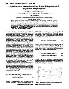
Fig. 1. Reconstruction with changed viewing angles.

#1670 - $15.00 US

(C) 2002 OSA

Received September 17, 2002; Revised October 10, 2002

4 November 2002 / Vol. 10, No. 22 / OPTICS EXPRESS 1251

As shown in Fig. 1, the transmittance τ ( x, y ) is vertically placed in the z=0 plane and the observation direction is along the z ′ axis. For simplicity we assume the viewing angle θ , the angle between the z ′ - axis and the original z- axis, to lie in the y-z plane. To reconstruct the real images with the given view angle, let us consider a plane wave Ei ( x, y ) with a unitary amplitude of Eo , shown black in Fig. 1, incident onto the hologram plane; however, the diffracted wave from the hologram is assumed to propagate along the new direction of θ . The observation plane xo − yo is assumed to be perpendicular to the z ′ axis. To obtain the reconstructed information on the observation plane xo − yo , let us first review the Rayleigh-Sommerfeld diffraction integral [9]: E ( xo , yo , zo ) =

iE0

λ

∫∫ τ ( x, y ) exp(iky sin θ )

exp[ikr ( x, y, xo , yo )] χ ( x, y, xo , yo )dxdy r ( x, y, xo , yo )

(1)

where λ is the wavelength, k is termed the wave number and given by k = 2π λ . χ ( x, y, xo , yo ) is the inclination factor, which will be approximately unitary if the Fresnel approximation is assumed. Thus it is omitted in the following equations. The constant before the integration can also be omitted. The first exponential term is introduced because of the angle between the normal plane of the inclined observation direction and the vertical hologram plane. From Fig. 1, we find that the distance r ( x, y, xo , yo ) is determined by r = ( zo − y sin θ )2 + ( xo − x) 2 + ( yo − y cos θ ) 2

(2)

If we introduce ro = ( zo + xo + yo ) [10], the above square root can be expanded in a power series and if only the first two lower order terms in the expanded series are considered, then Eq. (1) can be expressed as: 2

2

2



 ik 2 ( x + y 2 ) r 2  o 

E ( xo , yo , zo ) = exp(ikro ) ∫∫ τ ( x, y ) exp   ik × exp − [ xo x +  ro

yo y cos θ + ( zo

 − ro ) y sin θ ] dxdy 

(3)

ik 2 ( x + y 2 ) in the Eq. (3) depends on not only the coordinates of the observation 2ro plane but also the transmittance plane. An approximation can be introduced to simplify the calculation of Eq. (3):

The term

ik 2 ik 2 (x + y2 ) ≈ (x + y2 ) 2ro 2 zo

(4)

The boundary condition of the above equation is almost the same restriction as the Fresnel condition. Furthermore, The last term of Eq. (3) can be interpreted as the Fourier transform if we introduce the variables ξ and η as:

ξ= η=

#1670 - $15.00 US

(C) 2002 OSA

1

λ ro

xo

λ ro

[ yo cosθ + ( zo − ro ) sin θ ]

(5)

(6)

Received September 17, 2002; Revised October 10, 2002

4 November 2002 / Vol. 10, No. 22 / OPTICS EXPRESS 1252

From Eq. (4~6), we can finally simplify Eq. (3) as: 

 ik 2 ( x + y 2 )  exp [ −i 2π (ξ x + η y ) ] dxdy (7) 2 z  o  The above equation can be implemented with the fast Fourier transform (FFT) algorithm. It is very important to point out that the reconstructed information directly from Eq. (7) is actually related to the coordinate ( ξ , η ), which is a distorted coordinate from the original spatial coordinate ( xo , yo ) by Eq. (5,6). In other words, the samples obtained do not fit within the rectangular mesh in xo and yo . So a numerical interpolation (or coordinate transform) is needed to get the sampled values in the rectangular xo and yo . Thus the wave field with a changed viewing angle, θ , can be obtained. Specifically, if the viewing angle θ is equal to zero, then Eq. (7) can be further simplified as Fresnel diffraction formula (FDF) [1]. That is to say, FDF is only a special case of Eq. (7) when the viewing angle θ is selected as zero. Now let us discuss the reconstructed image quality and the space bandwidth product of the present system. As we know, the finest fringe spacing formed between the lights emanating from the opposite edges of the object is given by λ 2sin(α / 2) ≅ λ α , where α is the angular size of the object to be clearly reconstructed. In other words, the resolution p of the CCD camera can be given as p = λ α [4]. After digitization, we find that the spatial frequency bandwidth in the reconstructed image is approximately given by: ∆f xo = 1 δ xo ≅ Np λ zo , and ∆f yo = 1 δ yo ≅ Np cosθ λ zo (8)

E (ξ ,η, zo ) = exp(ikro ) ∫∫ τ ( x, y ) exp 

where N × N is the pixel number of a square CCD, δ xo and δ yo are the pixel sizes in the reconstructed image. From the above Equation we find that when the wavelength selected increases, the spatial frequency bandwidths in both directions decrease, and when the absolute value of the viewing angle θ increases, the spatial frequency bandwidth in the yo direction also decreases. For more detailed digitalization process of CCD-target for digital holography, readers can also refer to some earlier publications [1,4,11,12]. The space-bandwidth product of digital reconstruction in this paper is simply given as: P = α zo ∆f xo ⋅α zo ∆f yo ≅ N 2 cosθ (9) When the absolute value of the viewing angle θ increases, the space-bandwidth product decreases, which also means that the bigger the absolute viewing angle, the more information lost in the reconstructed image. Theoretically speaking, if the absolute viewing angle θ reaches 90 degrees, no information will be reconstructed. However, it might still seem strange that the viewing angle could be so large if it is compared with diffractive optical elements (DOE) used for beam shaping and splitting [13], where the fan-out angle θ is limited because of the limited DOE structure size. As we have mentioned, digital holography here means the technique to numerically reconstruct the digitally recorded hologram in a CCD-target by using of computers. Since the whole process of reconstruction is numerically performed, this technique in some sense could overcome the chemical or physical limitations of the reconstruction process in conventional holography or in other processes where the reconstruction need to be physically implemented. For example, wet film-developing process is necessary in conventional digital holography and the fan-out angle is limited in DOE. In digital holography, however, we could flexibly and virtually build up the numerical model of reconstruction to overcome some of these limitations to some extent, and effectively get the reconstructed images. For instance, if we want to reconstruct from the hologram with a small viewing angle θ , it would be reasonable to suppose the original incident beam, Ei ( x, y ) with a unitary amplitude

#1670 - $15.00 US

(C) 2002 OSA

Received September 17, 2002; Revised October 10, 2002

4 November 2002 / Vol. 10, No. 22 / OPTICS EXPRESS 1253

( Eo = 1 ), to vertically illuminate onto the hologram plane τ ( x, y ) . Here τ ( x, y ) is supposed to be a 2D transmittance, as shown in Fig. 1. It could be viewed as paraxial diffraction. However, if we want to reconstruct from the hologram with a larger viewing angle θ , because the reconstruction process is virtually and numerically performed, we could slightly change the reconstruction model, where we could assume that the incident beam is illuminated onto the hologram plane with the same inclined angle θ as the observation direction, as shown in Fig. 1 with a dashed blue color. But in this case we should make sure that the diffracted wave field behind the 2D hologram plane is still τ ( x, y ) . This process could also be viewed as paraxial diffraction (along z ′ axis). Thus it is feasible to numerically reconstruct from the hologram with a larger viewing angle θ (from z axis). However, as we have discussed, when the absolute value of the viewing angle θ increases, the spacebandwidth product of the system will decreases according to Eq. (9). When the absolute viewing angle θ reaches 90 degrees, no information will be reconstructed at all. From above we can see that, different reconstruction models are used according to different situations. This is to take advantage of the properties of numerical reconstruction, which could be flexibly, virtually and effectively implemented in a computer, but do not need to be physically implemented. 3. Numerical Simulations

x lo

li Hologram

Object

z

Reference beam

y

(a)

(b)

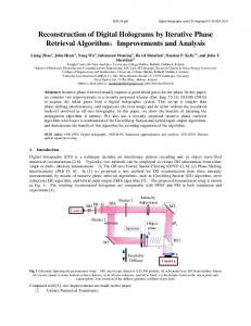
Fig. 2. (a) Recording and reconstructing a hologram; (b) Texture of the object.

In this section we implement some numerical experiments to verify the proposed algorithm for numerical reconstruction with variable viewing angles. The setup of the numerical experiment is shown as Fig. 2 (a), where in-line holography is assumed. The reference wave is shown as orange in the figure. Thus experimentally, we can extract the object information from multiple holograms with the phase-shifting technique [4]. Even for off-axis holography with an off-axis reference wave, as shown in Fig. 2 (a) with a dashed blue color, the object information could be extracted with a spectrum manipulating technique [6] if the off-axis angle is large enough, thus no twin-image and first order noise will appear in the reconstructed images. Let us first consider a vertically placed one-layer object. The texture of the object is shown in Fig. 2 (b), which contains some coaxial-circles. The distance between the object and the hologram plane is supposed to be lo = 1.2m , as shown in Fig. 2 (a). In the simulations, the wavelength in recording is supposed to be the same as that in reconstructing, which is set to be 632.8nm, so the real image of the object should lie at the position with li = 1.2m away from another side of the hologram plane. The object consists of 256×256 pixels with each pixel containing 256 gray levels in the process of numerical reconstruction and the total area of the object is set to be 13.9mm×13.9mm. Since in-line holography is assumed in this paper, the complex amplitude of the object on the hologram plane can be numerically calculated by

#1670 - $15.00 US

(C) 2002 OSA

Received September 17, 2002; Revised October 10, 2002

4 November 2002 / Vol. 10, No. 22 / OPTICS EXPRESS 1254

simulating four phase-shifted holograms [4]. The object information obtained after the phaseshifting process is shown as Fig. 3. Specifically, Fig. 3 (a) shows the magnitude of the complex object wave on the hologram plane and Fig. 3 (b) shows the phase image of the complex wave field. This wave information is used for numerical reconstruction.

(b)

(a)

Fig. 3. (a) Magnitude; (b) phase of the object wave on the hologram.

Now we use the algorithms proposed in this paper, Eqs. (5-7), for reconstruction. In our simulations linear interpolations are used. Fig. 4 shows the reconstruction results as a demo where the reconstructing distance is fixed as li = 1.2m and the viewing angle is changed from −75o to 75o . From the above demo we find that all the reconstructed frames have the same ratio in the vertical ξ direction; however, the horizontal η direction becomes more and more shrunk as the absolute viewing angle θ becomes more and more larger. This can be justified from Eqs. (5, 6) and (9) if we substitute different values for θ . Our simulations are carried out with the MATLAB 5.1 software in a P3-866 PC. The computation time of our proposed algorithm is about 16 seconds (to reconstruct a 256×256 image with one selected viewing angle), while the computation time for the Fresnel diffraction formula [1] is about 7 seconds.

η

ξ

Fig. 4. (GIF, 145KB) A demo of reconstructing the real object with fixed li = 1.2m but with changed viewing angles from −75o to 75o .

#1670 - $15.00 US

(C) 2002 OSA

Received September 17, 2002; Revised October 10, 2002

4 November 2002 / Vol. 10, No. 22 / OPTICS EXPRESS 1255

(a)

(b)

Fig. 5. (a) Texture of layer 1 at 1.0m; (b) Texture of the layer 2 at 1.2m.

Now let us consider another example of a two-layer object. The texture of layer 1 is shown as Fig. 5(a) and it is located with lo1 = 1.0m away from the hologram. Fig. 5(b) shows the texture of layer 2, which is located at the position of lo 2 = 1.2m . All the other parameters are the same as those used in the first demo. The complex object information of the new object on the hologram plane could be obtained by the same phase-shifting process, Fig. 6(a) shows the magnitude of the complex object wave and Fig. 6(b) shows the phase image of the complex wave field. Fig. 7(a) shows another demo where the viewing angle is fixed as θ = 45o but the reconstructing distance li is changed between 1.0m and 1.2m. From this demo we may find that the reconstructed image of layer 1 becomes much more vague since it gets far more out-of-focus as the reconstructing distance li is changed from 1.0m to 1.2m, and the reconstructed image of layer 2 becomes much clearer. Oppositely, if the reconstructing distance li is changed from 1.2m to 1.0m, then layer 1 in the reconstructed image will become clearer and clearer, however layer 2 will become more and more vague. Fig. 7(b) shows a third demo when both the viewing angle and the focal length are animatedly adjusted.

(a)

(b)

Fig. 6. (a) Magnitude; (b) phase of the object wave on the hologram.

#1670 - $15.00 US

(C) 2002 OSA

Received September 17, 2002; Revised October 10, 2002

4 November 2002 / Vol. 10, No. 22 / OPTICS EXPRESS 1256

(a)

(b)

Fig. 7. (a) (GIF, 1.54MB) A demo of reconstructing the real object with fixed viewing angle

θ = 45o but with changed focal length between 1.0m and 1.2m; (b) (GIF, 1.56MB) A demonstration with both the viewing angle and the focal length adjusted.

The above numerical simulations and demostrations clearly verify the effectiveness of using the proposed algorithm for numerical reconstruction with variable viewing angles. Both the focal lengths and the viewing angles could be changed in the reconstruction. 4. Conclusion This paper has explained a new method to reconstruct objects with changed viewing angles from a hologram within the Fresnel domain. The numerical reconstruction can be implemented by using the fast Fourier transform (FFT) algorithm. Some representative simulations and demonstrations are presented to validate our idea. Acknowledgment The authors would like to thank the Research Grants Council of Hong Kong for financial support of this work (Project No. HKUST6175/00E).

#1670 - $15.00 US

(C) 2002 OSA

Received September 17, 2002; Revised October 10, 2002

4 November 2002 / Vol. 10, No. 22 / OPTICS EXPRESS 1257