Numerical Simulation of Advective-Dispersive Multi ...

SUTRA—MS A Version of SUTRA Modified to Simulate Heat and Multiple-Solute Transport By Joseph D. Hughes and Ward E. Sanford

Open-File Report 2004-1207 U.S. Department of the Interior U.S. Geological Survey

Cover: Simulated double-diffusive convection using SUTRA-MS

SUTRA—MS A Version of SUTRA Modified to Simulate Heat and Multiple-Solute Transport By Joseph D. Hughes and Ward E. Sanford

Any use of trade, firm, or product names is for descriptive purposes only and does not imply endorsement by the U.S. Government

Open-File Report 2004-1207 U.S. Department of the Interior U.S. Geological Survey

U.S. Department of the Interior Gale A. Norton, Secretary U.S. Geological Survey Charles G. Groat, Director

U.S. Geological Survey, Reston, Virginia 2004

For product and ordering information: World Wide Web: http://www.usgs.gov/pubprod Telephone: 1-888-ASK-USGS

For more information on the USGS—the Federal source for science about the Earth, its natural and living resources, natural hazards, and the environment: World Wide Web: http://www.usgs.gov Telephone: 1-888-ASK-USGS

Although this report is in the public domain, permission must be secured from the individual copyright owners to reproduce any copyrighted material contained within this report.

Preface This report describes a complex computer model for analysis of fluid flow and multispecies and/or energy transport in subsurface systems. The user is cautioned that although the model will accurately reproduce the physics of flow and transport when used with proper discretization, it will give meaningful results only for well-posed problems based on sufficient supporting data.

This modified version of SUTRA has not been extensively beta tested beyond the example problems given in this report. Please report any problems to:

SUTRA-MS Support U.S. Geological Survey 431 National Center Reston, Virginia 20192 USA

Copies of the computer program are available free of charge from the U.S. Geological Survey’s web site:

http://water.usgs.gov/nrp/gwsoftware/sutra.html

SUTRA-MS Documentation

iii

Abstract A modified version of SUTRA is introduced that is capable of simulating variabledensity flow and transport of heat and multiple dissolved species through variably to fully saturated porous media. The original version of SUTRA is capable or simulating variable-density flow and transport of either heat or one dissolved species through variably to fully saturated porous media. This modified version was developed because of the importance of temperature and solute concentrations in many variable-density flow environments and the desire to implicitly simulate the transport of multiple dissolved species that may or may not affect fluid density. Users familiar with SUTRA should have little difficulty applying this version of SUTRA to multi-species transport problems. All modifications to SUTRA are general, the number of dissolved species that can be simulated is unrestricted by the program, any of the simulated species can affect fluid density and or viscosity, and simulation of heat transport is unrestricted by the number of simulated dissolved species. The model assumes density and viscosity are linear functions of solute concentration. For simulation of energy transport, the model assumes density is a linear function of temperature but the relation between temperature and viscosity is non-linear. A limitation of the current temperature-viscosity relationship is that it can be scaled only with user-specified parameters unless the code is modified and recompiled. However, alternative temperature-viscosity relationships can be easily incorporated in the source code. In addition to modifications that allow for multi-species transport, SUTRA has been modified to allow use of a spatially distributed solid matrix thermal conductivity and the option to use a geometric-mean approximation for bulk thermal conductivity that accounts for partial saturation. The geometric-mean approximation for bulk thermal conductivity was added because of supporting empirical evidence (Sass and others, 1971). In addition to modifications to the numerical algorithms in SUTRA, a number of optional functions have been added to minimize solution non-convergence, minimize user coding to simulate time-varying boundary conditions, reduce output file size, allow specification of hydraulic parameters using zones, and specify observation locations with spatial coordinates. A simplified automatic time-step algorithm has been added that reduces the time-step length, if the number of iterations exceeds a user-specified value, and can rerun time steps if the specified maximum number of iterations is exceeded. A simple algorithm has been added that allows any boundary condition to be time varying without the need for user-programmed functions, with the limitation that boundary conditions between the times when conditions are changed (at the beginning of stress periods) are not interpolated. Time steps are reduced to the minimum time step when new boundarycondition values are read. A simple technique has been implemented that permits the user to specify the exact time to write data to the nodal and elemental output files. Functionality has been added that allows hydraulic parameters to be specified using zones in order to reduce the memory requirements for large two- and three-dimensional simulations and to better facilitate the use of model-independent parameter-estimation codes (e.g., UCODE, Poeter and Hill, 1998; PEST, Doherty, 1994). A simple routine that


iv

allows observation locations to be specified using coordinates rather than node numbers also has been included. The modified version of SUTRA has retained all the functionality of the original SUTRA and can solve the flow and transport equations in either two or three dimensions. This version of SUTRA is backward compatible with standard two- and three-dimensional SUTRA single species input data sets. Multi-species data sets are different from standard data sets only when additional data are required for each simulated species. Three examples are presented that demonstrate the ability of the modified version of SUTRA to simulate multi-species transport. Two of these examples demonstrate the ability to simulate fluid density affected by more than one species, and one example shows several additional applications of the modified version of SUTRA. Where possible, the modified code is compared to observed data, the standard version of SUTRA (Voss and Provost, 2002), or other codes capable of simulating variable-density flow and heat and solute transport. Comparisons indicate the modified version of SUTRA is comparable to HST3D (Kipp, 1997) for a coupled heat and solute variable-densityflow problem, and is capable of simulating a coupled variable-density multi-species HeleShaw experiment.


v

Contents 1.0 Introduction................................................................................................................... 1 1.1 Purpose ................................................................................................................... 1 1.2 SUTRA Fundamentals and Previous Applications ................................................ 2 1.3 The Current Study .................................................................................................. 3 2.0 Physical-Mathematical Basis of SUTRA-MS Modifications ....................................... 5 2.1 General Mass-Balance Formulation ....................................................................... 5 2.1.1 Fluid Mass-Balance Equation .......................................................................... 5 2.1.2 Modified Form of the Fluid Mass- Balance Equation...................................... 6 2.1.3 Unified Energy- and Solute- Balance Equation ............................................... 7 2.1.4 Modified Form of the Unified Energy- and Solute- Balance Equation ......... 10 2.1.5 Modified Form of the Energy- Balance Equation used with Geometric-Mean Approximation for Bulk Thermal Conductivity ........................................... 12 3.0 Numerical Methods..................................................................................................... 15 3.1 Numerical Approximation of SUTRA-MS Fluid Mass Balance.......................... 15 3.2 Numerical Approximation of SUTRA-MS Unified Energy- and Solute-Balance Equation ............................................................................................................... 17 3.3 Temporal Evaluation of Adsorbate Mass Balance ............................................... 19 3.4 Solution Sequencing ............................................................................................. 22 4.0 Additional SUTRA-MS Options................................................................................. 25 4.1 Simple Time-Varying Boundary Conditions........................................................ 25 4.2 Specified User Output Times ............................................................................... 26 4.3 Simple Automatic Time-Stepping Algorithm ...................................................... 26 4.4 Specified Observation Locations.......................................................................... 28 4.5 Specification of Hydraulic Parameters Using Zones............................................ 28 5.0 SUTRA-MS Simulation Examples ............................................................................. 31 5.1 Density-dependent flow, heat transport, and solute transport, Solution for multicomponent fluid flow in a saline aquifer system ................................................. 31 5.1.1 Physical Setup ................................................................................................ 31 5.1.2 Simulation Setup ............................................................................................ 31 5.1.3 Parameters ...................................................................................................... 32 5.1.4 Boundary Conditions...................................................................................... 33 5.1.5 Initial Conditions............................................................................................ 34 5.1.6 Results ............................................................................................................ 34 5.2 Solution for double-diffusive finger convection induced by different fluid dispersivities and viscosities ................................................................................ 40 5.2.1 Physical Setup ................................................................................................ 40 5.2.2 Simulation Setup ............................................................................................ 40 5.2.3 Parameters ...................................................................................................... 41 5.2.4 Boundary Conditions...................................................................................... 42 5.2.5 Initial Conditions............................................................................................ 42 5.2.6 Results ............................................................................................................ 42


vi

5.3

Density-dependent flow with transport of a non-reactive tracer and zero-order production and transport of a solute to simulate ground- water age.................... 48 5.3.1 Physical Setup ................................................................................................ 48 5.3.2 Simulation Setup ............................................................................................ 49 5.3.3 Parameters ...................................................................................................... 50 5.3.4 Boundary Conditions...................................................................................... 50 5.3.5 Initial Conditions............................................................................................ 51 5.3.6 Results ............................................................................................................ 51 6.0 SUTRA-MS Data Input .............................................................................................. 55 6.1 SUTRA Input Data List........................................................................................ 55 6.2 General Format of the “.inp”, “.ics”, “.tbc”, “.otm”, “.ats”, “.sob”, and “.zon” Input Files ............................................................................................................ 57 6.3 List of Input Data for the “.inp” (Main Input) File............................................... 58 6.4 List of Input Data for “.ics” (Initial Conditions) File ......................................... 107 6.5 List of Input Data for “.tbc” (Simple Transient Boundary Conditions) File ...... 111 6.6 List of Input Data for “.otm” (Specified User Output Times) File..................... 119 6.7 List of Input Data for “.ats” (Simple Automatic Time-Stepping Algorithm) File ............................................................................................................................ 121 6.8 List of Input Data for “.sob” (Specified Observation Locations) File................ 123 6.9 List of Input Data for “.zon” (Node and Element zone parameters) File ........... 125 7.0 References................................................................................................................. 129 Appendix 1: Notation...................................................................................................... 132 Generic Units............................................................................................................... 133 Units 133 Special Notation .......................................................................................................... 133 Roman Lowercase ....................................................................................................... 134 Roman Uppercase........................................................................................................ 135 Greek Lowercase ......................................................................................................... 138 Greek Uppercase.......................................................................................................... 141

Figures Figure 2.1.1 Figure 4.5.1 Figure 5.1.1 Figure 5.1.2

Comparison of bulk thermal conductivity as a function of porosity, fluid saturation, and solid matrix thermal conductivity using a volumetric average and geometric-mean approximations........................................... 13 Simple representation of the differences in memory requirements for hydraulic parameters that are discretized by elements for SUTRA and SUTRA-MS using zones........................................................................... 29 Finite element mesh (υ=1) and pressure (gray), concentration (blue), and temperature (red) boundary conditions for Henry and Hilleke (1972) solution...................................................................................................... 32 Match of percent-seawater contours and the SUTRA-MS flow field for NΨ=3, NC=10, and υ=1 Henry and Hilleke numerical solution (0.5-percent


vii

Figure 5.1.3

Figure 5.1.4

Figure 5.1.5

Figure 5.2.1 Figure 5.2.2 Figure 5.2.3

Figure 5.2.4

Figure 5.2.5

Figure 5.3.1 Figure 5.3.2 Figure 5.3.3 Figure 5.3.4

seawater concentration only) (solid red line), HST3D code solution (dashed black line), and SUTRA-MS solution (colored).......................... 35 Match of percent-seawater contours and the SUTRA-MS flow field for NΨ=3, NC=10, and υ=0.10 Henry and Hilleke numerical solution (0.5percent seawater concentration only) (solid red line), HST3D code solution (dashed black line), and SUTRA-MS solution (colored)............ 36 Match of percent seawater contours, SUTRA-MS flow field, and match of isotherms for NΨ=3, NC=10, NT=1, and υ=1 Henry and Hilleke numerical solution (0.5 percent seawater concentration and isotherm only) (solid red line), HST3D code solution (dashed black line), and SUTRA solution (colored) with DM=8.333x10-6 and DT=8.333x10-5. ................................. 37 Match of percent-seawater contours, SUTRA-MS flow field, and match of isotherms for NΨ=3, NC=10, NT=1, and υ=0.10 Henry and Hilleke numerical solution (0.5-percent seawater concentration and isotherm only) (solid red line), HST3D code solution (dashed black line), and SUTRA solution (colored) with DM=8.333x10-8 and DT=8.333x10-7. ................... 38 Boundary and initial concentration conditions and finite-element mesh (every 16th element) used to simulate the Pringle and others (2002) HeleShaw experiment....................................................................................... 41 Absolute viscosity and fluid density relationships with NaCl and sucrose concentrations used in all SUTRA-MS simulations. Data arefrom Weast (1986). ....................................................................................................... 43 Observed results from Pringle and others (2002) at (A) t* = 4.06x10-5, (B) t* = 1.29x10-4, (C) t* = 3.96x10-4, (D) t* = 3.35x10-4, (E) t* = 4.35x10-4, (F) t* = 5.36x10-4, (G) t* = 6.03x10-4, and (H) t* = 7.37x10-4, (I) t* = 8.04x10-4, (J) t* = 1.04x10-3, (K) t* = 1.78x10-3, and (L) t* = 3.19x10-3. Color sequence black-blue-green-yellow-orange-red depicts normalized NaCl concentration from 0 to 1................................................................. 44 Simulated results SUTRA-MS results at (A) t* = 4.06x10-5, (B) t* = 1.29x10-4, (C) t* = 3.96x10-4, (D) t* = 3.35x10-4, (E) t* = 4.35x10-4, (F) t* = 5.36x10-4, (G) t* = 6.03x10-4, and (H) t* = 7.37x10-4, (I) t* = 8.04x10-4, (J) t* = 1.04x10-3, (K) t* = 1.78x10-3, and (L) t* = 3.19x10-3. Color sequence black-blue-green-yellow-orange-red depicts normalized dye concentrations from 0 to 1. ....................................................................... 45 Normalized vertical length, h*=h/H, and mass transfer across the center line, M*=M/Mo, as a function of time showing regions of steady growth for the original Hele-Shaw experiment (open gray circles) and the SUTRA-MS simulation (solid black circles and solid black line)............ 46 SUTRA finite-element mesh and boundary conditions............................. 49 Simulated percent-seawater contours from the 2D SUTRA-MS simulation after (A) 13.89 and (B) 27.78 days and the (C) 3D SUTRA-MS simulation after 27.78 days. ........................................................................................ 52 Simulated non-reactive tracer-concentration contours from (A) 2D SUTRA-MS, (B) 3D SUTRA-MS in XZ Plane at y=40 m, and (C) 3D SUTRA-MS in XY Plane at z=50 m......................................................... 53 Simulated ground-water age, in days, from SUTRA-MS. ........................ 54


viii

Figure 6.3.1

Figure 6.3.2

Minimization of bandwidth by careful numbering of nodes (Fig. 7.1 , Voss and Provost, 2002). In this 2D example, the same mesh has been numbered two different ways. In the first numbering scheme, the largest difference between node numbers in a single element is 15, giving a bandwidth of 1+2(15)=31. In the second numbering scheme, the largest difference between node numbers in a single element is 5, giving a bandwidth of 1+2(5)=11. The same principle applies to 3D meshes: the bandwidth equals one plus the maximum difference between node numbers in the element that contains the largest node number difference in the mesh. ................................................................................................... 88 Allocation of sources and boundary fluxes in equal-sized elements (Fig. B.1 , Voss and Provost, 2002). The top four panels pertain to 2D areal and 3D meshes. The bottom four panels pertain to 2D cross-sectional meshes. ................................................................................................................... 99

Tables

Table 5-1.

Discretization requirements for several aquifer aspect ratios (υ). See Appendix 1 for symbol definitions. .......................................................... 39


ix

1.0 Introduction Ground water in coastal environments, areas of high evaporation rates, and urban and industrial areas may have dissolved constituents that can affect fluid density. For example, in coastal aquifers, chloride concentrations can vary from 0 to 18,500 parts per thousands and have fluid densities ranging from 1,000 to 1,025 kg/m3 (kilograms per cubic meter) respectively. The range in fluid density of chloride concentrations from freshwater to seawater represents only a 2.5-percent increase in fluid density, but this small difference has been shown to have significant effects on ground-water-flow rates and patterns. Typically, multiple dissolved constituents are present in variable-density flow environments, but density variations usually can be related to a single constituent (i.e., chloride concentrations, total dissolved solids.) because of the positive correlation of each constituent with all the other constituents. Fluid temperature variations also affect fluid density. A 10°C increase in fluid temperature of freshwater results in a reduction in fluid density of approximately 4 kg/m3 (~0.5-percent reduction). The small change in fluid density over the range of fluid temperatures found in many shallow coastal systems allows temperature effects on fluid density to be ignored (Konikow and Reilly, 1999). In some natural systems, however, temperature variations have a significant effect on the flow system (e.g., hydrothermal systems, thick and/or deep aquifers). Similarly, fluid density may be a function of more than one dissolved species in some natural systems (Pringle and others, 2002). Furthermore, lateral and vertical aquifer heterogeneities in many natural systems cause the variable-density-flow system to be three dimensional in nature. A variety of numerical approaches have been used to simulate variable-density-flow problems (for a summary of available methods, see Sorak and Pinder, 1999). The methods that have been used include finite differences (e.g., INTERA, 1979), finite elements (e.g., Voss, 1984; Huyakorn and others, 1987; and Diersch, 1988), finite volumes (e.g., Kipp, 1987; Oldenburg and Pruess, 2000), analytical elements (Strack, 1995), and hybrid Eulerian-Lagrangian finite differences/finite elements (e.g., Sanford and Konikow, 1985; Yeh, 1987 and 1990). These approaches have included twodimensional and three-dimensional implementations of the available methods. This report describes a modified version of SUTRA capable of simulating variabledensity flow that is dependent on multiple dissolved constituents and temperature. SUTRA was selected for modification because of its wide use and modular nature that easily accommodates additional functionality. 1.1 Purpose The principal objectives of this report are to (1) introduce a general methodology that incorporates multiple dissolved species into the set of partial differential equations that describe variable-density flow and solute transport, (2) present a numerical model, SUTRA-MS (Saturated-Unsaturated Transport of Multiple Species), that utilizes this


1

methodology; (3) benchmark the computer code against existing numerical codes, previous numerical solutions, and experimental data; and (4) use SUTRA-MS results to demonstrate some of the processes that are important in the simultaneous transport of multiple species. 1.2 SUTRA Fundamentals and Previous Applications SUTRA uses a hybridized finite element and implicit finite-difference technique to solve the fluid mass-balance equation and unified energy- and solute- balance equation for variable-density, single-phase, saturated-unsaturated flow and single-species transport. Solving the equations in the time domain is accomplished by the implicit finite-difference method for non-flux terms (e.g., time derivatives and sources) in the region surrounding each specified node. All flux terms and associated parameters are discretized on an element basis and are solved by a modified Galerkin method. SUTRA uses bilinear quadrilateral elements in two dimensions and trilinear hexahedrons in three dimensions. SUTRA uses a modified form of the standard Galerkin finite-element method to allow for calculation of a consistent vertical velocity for each element. This is a significant but important modification for variable-density-flow simulations. In the standard Galerkin finite-element method, spurious vertical velocities are generated everywhere there is a vertical concentration gradient within the finite-element mesh, even if a hydrostatic pressure distribution is used (Voss, 1984; Voss and Souza, 1987). These spurious vertical velocities make it impossible to simulate a narrow transition zone between fluids with significant density differences (e.g., freshwater and seawater) with the standard finiteelement method, regardless of the specified dispersivity for the system. The modification used in SUTRA provides for a vertical velocity calculation within each finite element based on consistent spatial variability of the pressure gradient, ∇p, and the buoyancy term, ρg, in the variable-density form of Darcy's equation. SUTRA is a very general code that was developed using a modular coding convention (Voss, 1999). The modular nature of SUTRA has allowed it to be modified for specific projects and applications. Some of the modifications have included addition of equilibrium chemical reactions (Lewis and others, 1986), addition of kinetic reactions (e.g., Smith and others, 1997; Sahoo and others, 1998), and calculation of path lines (Cordes and Kinzelbach, 1992). SUTRA was initially released as a two-dimensional code that could solve constantdensity areal problems or constant- to variable-density cross-sectional problems. A 3D version of SUTRA was developed and tested in 1982. After running several test problems with the 3D version of SUTRA, the three-dimensional simulation capabilities were removed because of the limited computer resources that most users had access to in the early 1980s. Three-dimensional problems that were sufficiently discretized required access to super-computer facilities and had limited use to a small number of users (Voss, 1999). The decision to release a 2D version of SUTRA was appropriate and has allowed SUTRA to be widely used and applied to a variety of problems.


2

The 2D version of SUTRA has been applied to a number of problems including: (1) unsaturated flow studies; (2) contaminant/tracer studies; (3) energy-transport studies; (4) inverse modeling and optimization studies; (5) solute-dependent variable-density flow; and (6) temperature- dependent variable-density flow. A summary of published SUTRA applications is given in Voss (1999). Recent improvements in computer processors and associated hardware have allowed an updated and improved 3D version of SUTRA to be released (Voss and Provost, 2002). Advances in techniques to solve numerical problems have allowed incorporation of robust, iterative solvers in the 3D version of SUTRA and made developing and solving 3D variable-density-flow problems practical. The 3D version of SUTRA retains all the original functionality of the 2D version and has been applied successfully to contaminanttransport problems and variable-density-flow problems. 1.3 The Current Study This report outlines the development of and some applications for a modified version of SUTRA: SUTRA-MS. The principal modification in SUTRA-MS is an extension of existing numerical methods to solve for the transport of multiple species and allow for dependence of density and viscosity on any of the simulated species. All the features of the original version of SUTRA have been retained in SUTRA-MS, including variably saturated to fully saturated flow, advection, and production and decay of simulated species. Other modifications include: • capability to simulate a spatially varying solid matrix thermal conductivity, • capability to use either a volumetric average or geometric-mean approximation for bulk thermal conductivity, • ability to simulate simple time-varying boundary conditions that do not need to be user programmed, • capability to output nodal- and element-simulation data at user-specified times, • ability to use a simplified automatic time-stepping algorithm to adjust time steps based on solution convergence, including the capability to rerun a time step if user-specified parameters are not achieved, • ability to enter observation locations using spatial coordinates instead of node numbers, • capability to specify hydraulic parameters using zones in order to reduce memory requirements for large two- and three-dimensional problems and facilitate the use of generic parameter-estimation codes, and • use of Fortran 95 intrinsic functions or programming standards where beneficial to program execution times, maintainability, or source-code clarity. The current modifications do not place an arbitrary limit on the number of species that can be simulated. The number of species that can be simulated is a function of the problem size and the amount of available random access memory (RAM). Furthermore,


3

the modifications are such that more complicated relationships between solute concentration and system state (e.g., density, etc.) can be easily incorporated.


4

2 .0 Physical-Mathematical Basis of SUTRA-MS Modifications This section summarizes the governing equations used in SUTRA to simulate fluid flow and solute transport in constant-density and variable-density environments. The modifications to the original equations are summarized here to provide background for the numerical implementation discussed in Section 3. To allow for simulation of multispecies transport with possible fluid-density and viscosity dependence on solute concentrations and temperature, all equations that include fluid density, fluid viscosity, velocity-dependent dispersion, molecular dispersion, thermal conductivity, solute adsorption, solute production and decay, solute or temperature boundary conditions, solute concentrations, or temperature require modification. Notations used in the equations are explained after their first use and also are summarized in appendix 1. 2.1 General Mass-Balance Formulation SUTRA-MS is a modified version of SUTRA capable of simulating unsaturated to saturated, variable-density fluid flow dependent on the transport of heat and multiple dissolved species. Because the modifications required to allow SUTRA to simulate transport of more than one species, including temperature, may affect both the flow and transport equations solved by SUTRA, a brief overview of the general mass-balance equations used in SUTRA is given below. A more complete discussion of SUTRA fundamentals is given in Voss and Provost (2002). 2.1.1 Fluid Mass-Balance Equation The fluid mass-balance equation, which is usually referred to as the ground-water-flow equation, is ( S w ρS op + ε

⎡⎛ kk ∂S w ∂p ∂p ∂U ) + (εS w ) − ∇ ⋅ ⎢⎜⎜ r ∂p ∂t ∂U ∂t ⎣⎝ µ

⎤ ⎞ ⎟⎟ ⋅ (∇p − ρg )⎥ = Q p ⎠ ⎦

where Sw is the water saturation [-], ε is the porosity [-], p is the fluid pressure [M/LT2], t is time [T], U is either temperature [°C] or solute mass fraction [Msolute/Mfluid], k is the permeability tensor [L2], kr is the relative permeability for unsaturated flow [-], µ is the fluid viscosity [M/LT], ρ is the fluid density [M/L3], g is the gravitational vector [L/T2], Qp is a fluid mass source [M/L3T], and Sop is the specific pressure storativity [M/LT2]-1. Specific pressure storativity, Sop, is defined as


5

Eq. 2.1

S op = (1 − ε )α + εβ

where

Eq. 2.2

α is the compressibility of the porous matrix [M/LT2]-1, and β is the compressibility of the fluid [M/LT2]-1.

2.1.2 Modified Form of the Fluid Mass- Balance Equation In SUTRA-MS, the generalized fluid mass-balance equation (eq. 2.1) has been modified to allow for more than one species to affect fluid density. The modified fluid massbalance equation is ( S w ρS op + ε ⎡⎛ kk − ∇ ⋅ ⎢⎜⎜ r ⎣⎝ µ

⎛ NS ∂p ∂C k ∂S w ∂p ∂p ∂T ⎞ ⎟ +τ + εS w ⎜⎜ ) ∂T ∂t ⎟⎠ ∂p ∂t ⎝ k =1 ∂C k ∂t

∑

⎤ ⎞ ⎟⎟ ⋅ (∇p − ρg )⎥ = Q p ⎠ ⎦

Eq. 2.3

where NS is the number of dissolved species simulated, τ = 1 if heat transport is being simulated and τ = 0 if otherwise, Ck is the solute concentration of species k [Msolute/Mfluid], and T is the temperature of the solution [°C]. The modified form of the fluid density, ρ, equation used in SUTRA-MS is ∂ρ (C k − C ko ) + τ ∂ρ (T − To ) ∂T k =1 ∂C k NS

ρ = ρo + ∑

where

Eq. 2.4

ρo is the fluid density at the base concentration of all simulated species at the base solute concentrations and temperature [Msolute/L3solute], Cko is the base solute mass fraction of species k [Msolute/Mfluid], and To is the base temperature [°C].

Equation 2.4 assumes ∂ρ/∂Ck and ∂ρ/∂T are constant over the range of simulated mass fractions, and temperatures and density relationships are linear and additive. This is an ad-hoc relationship but it is consistent with relationships used by others for similar applications (e.g., Kipp, 1987). This ad-hoc relationship should be evaluated prior to use and modified if it is determined to be inappropriate for a particular application. The modified form of the fluid viscosity, µ, used in SUTRA-MS is


6

∂µ (C k − C ko ) k =1 ∂C k NS

µ = µ o (T ) + ∑

Eq. 2.5

where

µο(Τ) =

a user-defined base fluid viscosity for isothermal flow at the base mass fraction for each species [M/LT], or

(

)

⎛ 248.37 ⎞ ⎜ ⎟

239.4x10 −7 10 ⎝ T +133.15 ⎠ for temperature-dependent flow [M/LT].

If temperature-dependent flow is simulated, the units of µo(T) can be converted to those desired using a scaling factor in the program input data. Equation 2.5 assumes ∂µ /∂Ck is constant over the range of simulated mass fractions, the specified non-linear viscositytemperature relationship is appropriate for the range of simulated temperatures, and viscosity mass-fraction relationships are linear and are not affected by species or temperature interaction. This is an ad-hoc relationship based on the concentration-density relationship described above. This ad-hoc relationship should be evaluated prior to use and modified if it is determined to be inappropriate for a particular application. 2.1.3 Unified Energy- and Solute- Balance Equation SUTRA uses a unified energy- and solute-balance equation to solve both energy and solute transport. A unified energy-solute balance is possible because of the similarity of the mechanisms affecting the fluxes of energy and solute mass in solution when energy and solute transport equations are formulated in terms of energy per unit volume and total species mass per unit volume, respectively. In fact, of the transport processes represented in SUTRA, only non-linear sorption processes and first-order production of solute and adsorbate mass have no analogy in energy transport. A mass-conservative form of the unified balance equation is solved by SUTRA and is derived from a general form of the equation in Voss and Provost (2002). The derivation of the mass-conservative form of the unified balance equation involves removing terms accounted for in the fluid mass-balance equation (fluid saturation and pressure-change contribution to energy and solute balances) and terms related to change in the solid matrix density with time. The reader is referred to Voss and Provost (2002) for a more complete description of the derivation of the mass-conservative form of the unified balance equation. The mass-conservative form of the unified balance equation is ∂U + ε Sw ρcw v ⋅ ∇U ⎡⎣ε Sw ρcw + (1 − ε ) ρs cs ⎤⎦ ∂t

{

−∇ ⋅ ρcw ⎡⎣ε Sw (σ w I + D ) + (1 − ε )σ s I ⎤⎦ ⋅ ∇U

(

)

}

Eq. 2.6

= Q p cw U * − U + ε Sw ργ 1wU + (1 − ε ) ρsγ 1sU s + ε Sw ργ ow + (1 − ε ) ρsγ os


7

where cw is the fluid specific heat [E/M°C] for heat transport or one (1) for solute transport, ρs is the density of the solid matrix [M/L3], cs is solid matrix specific heat [E/M°C] for heat transport or the sorption coefficient [-] for solute transport, v is the fluid velocity [L/T], σw is the fluid thermal diffusivity [L2/T] for heat transport or molecular diffusivity (Dm) for solute transport [L2/T], I is the identity tensor, D is the dispersion tensor [L2/T] for heat or solute transport, σs is the solid matrix thermal diffusivity [L2/T] for heat transport or zero (0) for solute transport, U* is the temperature of the source fluid [°C] for heat transport or the solute concentration of the source fluid [M solute/M fluid] for solute transport, w γ 1 is zero (0) for heat transport or the first-order mass-production rate of solute [T-1] for solute transport, γ 1s is zero (0) for heat transport or the first-order mass-production rate of adsorbate [T-1] for solute transport, Us is the specific energy content of the solid matrix [E/M] for heat transport (but does not contribute to the unified balance equation because γ 1s is zero (0)) or the concentration of the adsorbate on the solid matrix (Cs) for solute transport [M adsorbate/M solid matrix], γ 0w is the zero-order energy-production rate in the fluid [E/MT] for heat transport or the zero-order mass-production rate of solute [(M solute/M fluid)T-1] for solute transport, and s γ 0 is the zero-order energy-production rate in the solid matrix [E/MT] for heat transport or the zero-order mass-production rate of adsorbate [(M adsorbate/M solid matrix and adsorbate)T-1] for solute transport. Fluid thermal diffusivity, σw, in equation. 2.6 is defined as λ σw = w ρc w where

λw is the fluid thermal conductivity [E/TL°C].

Solid matrix thermal diffusivity, σs, in equationq. 2.6 is defined as λ σs = s ρc w where

Eq. 2.7

λs is the solid thermal conductivity [E/TL°C].


8

Eq. 2.8

Three equilibrium sorption models, which specify cs in equation. 2.6, are possible in SUTRA. These three sorption models assume fluid density is constant. The three sorption models are Linear equilibrium sorption model U s = (χ 1 ρ o )U

Eq. 2.9a

∂U s ∂U = (χ 1 ρ o ) ∂t ∂t

Eq. 2.9b

cs = κ 1 = χ1 ρ o

Eq. 2.9c

where

χ1 is the linear distribution coefficient [L3 fluid/M solid and adsorbate], and

κ1is the first general sorption coefficient. Freundlich equilibrium sorption model U s = χ 1 ( ρ oU )

⎛ 1 ⎞ ⎟ ⎜ ⎜χ ⎟ ⎝ 2⎠

Eq. 2.10a ⎛ 1− χ 2 ⎞ ⎟ χ 2 ⎟⎠

⎜ ⎜ ⎛χ ⎞ ∂U s c s = ⎜⎜ 1 ⎟⎟(ρ oU ) ⎝ dt ⎝ χ2 ⎠

⎛χ c s = κ 1 = ⎜⎜ 1 ⎝ χ2

where

⎞ ⎟⎟ ρ o ⎠

⎛ 1 ⎞ ⎜ ⎟ ⎜χ ⎟ ⎝ 2⎠

U

ρo

∂U ∂t

⎛ 1− χ 2 ⎞ ⎜ ⎟ ⎜ χ ⎟ ⎝ 2 ⎠

Eq. 2.10 b

Eq. 2.10c

χ1 is a Freundlich distribution coefficient [L3 fluid/M solid and adsorbate],

and χ2 is the Freundlich coefficient [-]. Langmuir equilibrium sorption model Us =

χ 1 ( ρ oU ) 1 + χ 2 (ρ oU )

Eq. 2.11a

∂U s χ1 ρ o ∂U = 2 ∂t (1 + χ 2 ρ oU ) ∂t


Eq. 2.11b

9

cs = κ 1 =

where

χ1 ρ o (1 + χ 2 ρ oU )2

Eq. 2.11 c

χ1 is a Langmuir distribution coefficient [L3 fluid/M solid and adsorbate], and

χ2 is the Langmuir coefficient [-].

2.1.4 Modified Form of the Unified Energy- and Solute- Balance Equation In SUTRA-MS, the mass-conservative form of the unified balance equation (eq. 2.6) has been modified to allow for simultaneous, sequential simulation of more than one species. The three forms of the sorption equations (eqs. 2.9, 2.10, and 2.11) also have been modified to allow simulation of multiple species, each of which can have different adsorption isotherms. The modified mass-conservative form of the unified balance equation is

[εS w ρc wk + (1 − ε )ρ s c sk ] ∂U k + εS w ρc wk v ⋅ ∇U k ∂t − ∇ ⋅ {ρc wk [εS w (σ wk I + D k ) + (1 − ε )σ sk I ] ⋅ ∇U k } = Q p c wk (U k* − U k ) + εS w ρ (γ 1w )k U k + (1 − ε )ρ s (γ 1s )k U sk + εS w ρ (γ ow )k + (1 − ε )ρ s (γ os )k

Eq. 2.12

where cwk is the fluid specific heat [E/M°C] for heat transport if species k is “ENERGY” or one (1) for solute transport of species k, csk is the solid matrix specific heat [E/M°C] for heat transport if species k is “ENERGY” or the sorption coefficient [-] for solute transport of species k , Uk is either fluid temperature [°C] if species k is “ENERGY” or concentration [M solute/M fluid] for solute transport of species k, Dk is the thermal-dispersion tensor [L2/T] if species k is “ENERGY” or the solute transport dispersion tensor or [L2/T] of species k, σsk is the solid matrix thermal diffusivity [L2/T] if species k is “ENERGY” or zero (0) for solute transport of species k, σwk is the fluid thermal diffusivity [L2/T] if species k is “ENERGY” or molecular diffusivity, DM, [L2/T] of species k, U k* is the temperature of the source fluid [°C] if species k is “ENERGY” or the solute concentration of the source fluid [M solute/M fluid] for species k, γ 1w k is zero (0) if species k is “ENERGY” or the first-order mass-production rate of species k solute [T-1],

( )


10

(γ ) is zero (0) if species k is “ENERGY” or the first-order mass-production rate s 1 k

of species k adsorbate [T-1], Usk is the specific energy content of the solid matrix [E/M] if species k is “ENERGY” (does not contribute to the unified balance equation because (γ 1s )n is zero (0)) or the concentration of species k adsorbate on the solid matrix [M solute/M solid matrix], γ 0w k is the zero-order energy-production rate in the fluid [E/MT] if species k is “ENERGY” or zero-order mass-production rate of species k solute [(M solute/M fluid)T-1], and γ 0s k is the zero-order energy-production rate in the solid matrix [E/MT] if species k is “ENERGY” or zero-order mass-production rate of species k adsorbate [(M adsorbate/M solid matrix and adsorbate)T-1].

( ) ( )

The modified forms of the three equilibrium models, which specify csk in equation . 2.12, are Linear equilibrium sorption model c sk = κ 1k = χ 1k ρ o

where

Eq. 2.13

χ1k is the linear distribution coefficient [L3 fluid/M solid and adsorbate] of species k, and

κ 1k is the first general sorption coefficient of species k.

Freundlich equilibrium sorption model c sk = κ 1k

where

⎛χ = ⎜⎜ 1k ⎝ χ 2k

⎞ ⎟⎟ ρ o ⎠

⎛ 1 ⎜ ⎜χ ⎝ 2k

⎞ ⎟ ⎟ ⎠

Uk

⎛ 1− χ 2 k ⎜ ⎜ χ ⎝ 2k

⎞ ⎟ ⎟ ⎠

Eq. 2.14

χ1k is a Freundlich distribution coefficient [L3 fluid/M solid and adsorbate] for species k, and χ2k is the Freundlich coefficient [-] for species k.

Langmuir equilibrium sorption model c sk = κ 1k =


χ 1k ρ o

Eq. 2.15

(1 + χ 2k ρ oU k )2

11

where

χ1k is a Langmuir distribution coefficient [L3 fluid/M solid and adsorbate] for species k, and χ2k is the Langmuir coefficient [-] for species k.

Equations 2.13 through 2.15 also assume fluid density, ρo, is constant and aqueous reactions among the simulated species are limited and can be ignored. The appropriateness of this assumption should be evaluated before using SUTRA-MS for a particular application. Although sorption of multiple species has been implemented in a simple fashion, SUTRA-MS is modular and a more sophisticated method of sorption could be implemented in the current program if required. More sophisticated sorption methods that account for aqueous interactions among dissolved species that also adsorb to the solid matrix have been implemented in a constant-density version of SUTRA, SATRA-CHEM (Lewis and others, 1986), and could be used as a template for modifying SUTRA-MS. 2.1.5 Modified Form of the Energy- Balance Equation used with GeometricMean Approximation for Bulk Thermal Conductivity The thermal conductivity of upper crustal materials generally varies by less than a factor of 5 whereas permeability can vary over 16 orders of magnitude (Ingebritsen and Sanford, 1998). SUTRA uses a volumetric average approximation for bulk thermal conductivity (eq. 2.16). λ ≡ εS w λ w + (1 − ε )λ s

where

Eq. 2.16

λ is the bulk thermal conductivity.

Empirical evidence shows that bulk thermal conductivity is well modeled using the geometric mean of the rock conductivity and fluid conductivity (Sass and others, 1971). The geometric-mean approximation of bulk thermal conductivity modified for variably saturated media is

(

)

ε

λ ≡ λ A (1− Sw) λ w Sw λ(s1−ε )

where

Eq. 2.17

λA is the thermal conductivity of air.

The thermal conductivity of air is a function of temperature but varies by less that 15percent (0.025 to 0.027 W/m°C) over typical appropriate temperature ranges for SUTRA-MS simulations (between 5 and 50°C). Because the thermal conductivity of air is approximately 1 to 2 orders of magnitude less that the thermal conductivity of water and geologic materials, respectively, a constant value of 0.026 W/m°C is used in bulk thermal-conductivity calculations when the geometric-mean approximation is used.


12

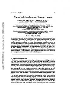
Use of a geometric-mean approximation for bulk thermal conductivity typically results in a reduction of approximately 15 percent in bulk thermal conductivity from volumetric average bulk thermal conductivities at typical porosities and solid matrix thermal conductivities. The differences in bulk thermal conductivities calculated using the volumetric average and geometric-mean approximations generally increase with increasing porosity and/or decreasing fluid saturation (fig. 2.1.1 ). λB = (λA(1-SW)λWSW)ε λS(1-ε)

λB = εSWλW+(1-ε)λS 10

λs=5

Bulk Thermal Conductivity (W/moC)


10

1

0.1

0.01 0.2

0.4 0.6 Porosity

0.8

0.1

1

0

0.2

0.4 0.6 Porosity

10

λs=4



10

1

0.1

0.01

0.8

1

λs=4

1

0.1

0.01 0

0.2

0.4 0.6 Porosity

10

0.8

1

0

0.2

0.4 0.6 Porosity

10

λs=3



1

0.01 0

1

0.1

0.01

0.8

1

λs=3

Fluid Saturation Sw 1.0 0.8 0.6 0.4 0.2 0.0

1

0.1

0.01 0

Figure 2.1.1

λs=5

0.2

0.4 0.6 Porosity

0.8

1

0

0.2

0.4 0.6 Porosity

0.8

1

Comparison of bulk thermal conductivity as a function of porosity, fluid saturation, and solid matrix thermal conductivity using a volumetric average and geometric-mean approximations.

When the geometric mean thermal-conductivity approximation is used, bulk thermal diffusivity in equation. 2.6 is defined as


13

(

)

⎛ λ1− S w λ S w ε λ(1−ε ) ⎞ s w A ⎟ ⎜ ⎟ ρc w ⎝ ⎠

σ bg = ⎜

where

Eq. 2.18

σbg is the bulk thermal diffusivity [L2/T].

Equation 2.12 is modified for energy transport in the following manner when using a geometric-mean approximation for bulk thermal conductivity

[εS w ρc wk + (1 − ε )ρ s c sk ] ∂U k

{

− ∇ ⋅ ρc wk

(

+ εS w ρc wk v ⋅ ∇U k ∂t σ bgk I + εS w D k ⋅ ∇U k

[

)

] } ρ (γ ) U (γ )

= Q p c wk U k* − U k + εS w

( )

+ εS w ρ γ

where

w o k

+ (1 − ε )ρ s

w 1 k

k

( )

+ (1 − ε )ρ s γ 1s k U sk

Eq. 2.19

s o k

σbgk is the bulk thermal diffusivity [L2/T] if species k is “ENERGY” or molecular diffusivity, DM, [L2/T] of species


14

3 .0 Numerical Methods As a result of the modified fluid mass-balance equation (eq. 2.3) and the modified unified energy- and solute--balance equation (eq. 2.12), the discretized, weighted-residual relations approximating these equations have been modified in SUTRA-MS. Complete development of the discretized, weighted residual approximations of equations 2.1 and 2.6 are given in Voss and Provost (2002). Explanation of the notation used in the equations developed in Section 3 is given after its first use in an equation and also is summarized in appendix 1. 3.1 Numerical Approximation of SUTRA-MS Fluid Mass Balance The modified unified energy- and solute-balance equation (eq. 2.3) is approximated numerically through nodewise, elementwise, and cellwise discretization. The weighted residual relation that allow for solution of pressures at nodes at the end of the present time step is ⎡⎛ AFi n +1δ ij ⎢⎜ ⎜ ∆t n +1 j =1 ⎢ ⎣⎝

NN

∑

⎤ ⎞ ⎟ + BF n +1 + ν δ ⎥ p n +1 ij pi ij j ⎟ ⎥⎦ ⎠

n +1 = Qin +1 + ν pi p BC i

n NS +τ ⎡ ⎤ ⎛ AF n +1 ⎞ n +1 ⎛ dU ik ⎞ CF + DFi (n +1)* + ⎜⎜ i ⎟⎟ p in + ⎢ ik ⎜ ⎟ ⎥ i = 1, NN ⎝ dt ⎠ ⎥⎦ k =1 ⎢ ⎝ ∆t n +1 ⎠ ⎣

∑ (

Eq. 3.1

)

where

∂S ⎞ ⎛ AFi n +1 = ⎜⎜ S w ρS op + ερ w ⎟⎟ Vi ∂p ⎠ i ⎝ ⎛ ∂ρ CFikn +1 = ⎜⎜ εS w ∂U k ⎝

Eq. 3.2

⎞ ⎟⎟ Vi ⎠i

⎧⎪⎡ BFijn +1 = ∫ ∫ ∫ ⎨⎢ k L x y z ⎪ ⎩⎣ ⎧⎪⎡ DFi (n +1)* = ∫ ∫ ∫ ⎨⎢ k L x y z ⎪ ⎩⎣

Eq. 3.3

⎤ ⎫⎪ ⎛ kr ρ ⎞ ⎟⎟ ⋅ ∇φ j ⎥ ⎬ ⋅ ∇ω i dz dy dx ⎜⎜ ⎝ µ ⎠ ⎦ ⎪⎭ ⎛ kr ρ ⎞ ⎟⎟ ⋅ ρg ⎜⎜ ⎝ µ ⎠

δij is the Kronecker delta:

*

⎤ ⎫⎪ ⎥ ⎬ ⋅ ∇ω i dz dy dx ⎦ ⎪⎭

⎧0 if i ≠ j ⎩1 if i = j ∆t n+1 is the length of the current time step,

δ ij = ⎨


15

Eq. 3.4

Eq. 3.5

pin+1 is the pressure in cell i at the end of the current time step, pin is the pressure in cell i at the end of the previous time step, Qin+1 is the total mass source [M/T] to cell i for the current time step,

νpi is the pressure-based conductance [LT] for the specified pressure source in cell i (zero (0) for all nodes that are not specified pressure nodes), n +1 is the specified pressure in cell i,(zero (0) for all nodes that are not specified p BC i

pressure nodes), n ⎛ dU ik ⎞ ⎜ ⎟ is the rate of change in solute concentration of species k in cell i during ⎝ dt ⎠

⎛ U n − U ikn −1 ⎞ ⎟, the previous time step ⎜⎜ ik ⎟ ∆ t n ⎝ ⎠ Vi is the volume of cell i, φj is the symmetric bilinear (2D) or trilinear (3D) basis function in global coordinates for node j , ωi is the asymmetric weighting function in global coordinates for node i, k L is the permeability tensor [L2] that is discretized elementwise, and

ρg

*

is an elementwise discretization of (ρg) that is consistent with the

discretization of ∇p. For two-dimensional simulations, equations. 3.4 and 3.5 are written as

⎧⎪⎡ BFij = ∫ ∫ ⎨⎢ k L x y ⎪ ⎩⎣

⎤ ⎫⎪ ⎛ kr ρ ⎞ ⎟⎟ ⋅ ∇φ j ⎥ ⎬ ⋅ ∇ω i B dy dx ⎜⎜ ⎝ µ ⎠ ⎦ ⎪⎭

⎧⎪⎡ DFi = ∫ ∫ ⎨⎢ k L x y ⎪ ⎩⎣

⎛ kr ρ ⎞ ⎟⎟ ⋅ ρg ⎜⎜ ⎝ µ ⎠

*

⎤ ⎫⎪ ⎥ ⎬ ⋅ ∇ω i B dy dx ⎦ ⎪⎭

Eq. 3.6

Eq. 3.7

where the thickness of the mesh, B(x,y), is evaluated at each Gauss point according to the following nodewise discretization NN

B ( x, y ) = ∑ B i φ i ( x, y )

Eq. 3.8

i =1

The superscript involving (n) or (n+1) indicates the value is evaluated at the end of the previous time step and the end of the current time step, respectively. The only integrals requiring Gaussian integration are BFij and DFij. These integrals are evaluated in an element-by-element manner in the SUTRA-MS subroutine ELEMN2 (for


16

2D) or ELEMEN3 (for 3D). The other terms, except for those involving νpi, are evaluated cellwise (one for each node) by the SUTRA-MS subroutine NODAL. The specified pressure terms are evaluated by subroutine BC. Equation 3.1 is assembled for each node in the model mesh in a given time step and is solved using either Gaussian elimination or an iterative solver. For the iterative solvers, an approximate solution is achieved when the residual error (summation of eq. 3.1 for each node) is less than a user-specified convergence criteria. Details of the flow and transport solution scheme used in SUTRAMS is given in Section 3.4.

3.2

Numerical Approximation of SUTRA-MS Unified Energy- and SoluteBalance Equation The modified unified energy- and solute-balance equation (eq. 2.12) is approximated numerically through nodewise, elementwise, and cellwise discretization. The weighted residual relations that allow for solution of concentration or temperature at nodes at the end of the present time step are ⎧ NN ⎡⎛ AT n +1δ ⎞ ⎫ ⎤ n n +1 ⎪ ⎪ ⎢⎜ ik ij ⎟ + DTijk(n +1)* + BTijkn +1 + ν U + GTikn +1 + G s TLnik+1 + Qin +1 + Q BC ⎥ c U δ wk ij ik ik i ⎪ j =1 ⎢⎜⎝ ∆t n +1 ⎟⎠ ⎪ ⎥⎦ ⎣ ⎪ ⎪ ⎪ ⎪ n +1 n +1 n +1 n +1 n n +1 ( n +1)* = + + + Ψ + c Q U Q U U ET ν ⎨ wk i ⎬ k = 1, NS + τ ik IN ik U ik UBCik BCik BCi ik ⎪ ⎪ ⎛ ATikn +1 ⎞ n ⎪ ⎪ n +1 ⎜ ⎟U ik i = 1, NN ⎪+ G s TRik + ⎜ ∆t ⎪ ⎟ ⎝ n +1 ⎠ ⎪⎩ ⎪⎭

[

∑

(

(

) ]

)

Eq. 3.9

where

ATikn +1 = (εS w ρc wk + (1 − ε )ρ s c sk )i Vi

(S w ρ )c wk

∫ ∫ ∫ ⎡⎢⎣

ε

[ε

(

DTijk(n +1)* =

x y z

BTijkn +1 =

∫ ∫ ∫ {ρc

wk

S w σ wk I + D k

v

*

Eq. 3.10

⋅ ∇φ j ⎤ω i dz dy dx ⎥⎦

) + (1 −

ε

)

Eq. 3.11

] }

σ skL I ⋅ ∇φ j ⋅ ∇φ i dz dy dx

Eq. 3.12

x y z

(

)

GTikn +1 = εS w ργ 1wk i Vi

Eq. 3.13

(

)

(

)

G s TLnik+1 = (1 − ε )ρ s γ 1sk s Lk i Vi

Eq. 3.14

Gs TRikn +1 = (1 − ε )ρ s γ 1sk s Rk i Vi n +1 ΨIN = ik

∫

Eq. 3.15

[

ρc wk εS w (σ wk I + D k ) + (1 − ε ) σ sL I

Γ


17

]

n +1

⋅ n φ i dΓ

Eq. 3.16

(

)

ETikn +1 = εS w ργ 0wk + (1 − ε )ρ s γ 0sk i Vi

Eq. 3.17

U ikn+1 is the concentration or temperature of species k in cell i at the end of the

current time step, U ikn is the concentration or temperature of species k in cell i at the end of the

previous time step, n is Q BC i

the total solute [M/MT] or energy source [E/T] of species k to cell i due to a specified pressure for the previous time step,

νUik is the concentration [LT] or temperature-based conductance [LT] for the

specified concentration or temperature of species k in cell i (zero (0) for all nodes that are not specified pressure nodes) for the current time step,

sLk is the sorption isotherm contribution to the left-hand side of equation 3.9 for species k (discussed further in section 3.3), sRk is the sorption isotherm contribution to the right-hand side of equation 3.9 for species k (discussed further in section 3.3), n +1 U BC ik

is the specified concentration or temperature of species k in cell i for inflow due to a specified pressure (zero (0) for all nodes that are not specified pressure nodes) for the current time step,

n is the unit outward normal vector,

φj is the symmetric bilinear (2D) or trilinear (3D) basis function in global coordinates for node j,

Γ is the external boundary area of the simulated region [L2], σ sL

is the solid matrix thermal diffusivity [L2/T] that is discretized

elementwise, and

ε is an elementwise discretization of porosity. For two-dimensional simulations, equations 3.11 and 3.12 reduce to DTijk(n +1)* =

∫ ∫ ⎡⎢⎣

ε

(S w ρ )c wk

x y

BTijkn +1 =

∫ ∫ {ρc

wk

[ε

(

S w σ wk I + D k

v

*

⋅ ∇φ j ⎤ω i B dy dx ⎥⎦

) + (1 −

ε

)

Eq. 3.18

] }

σ skL I ⋅ ∇φ j ⋅ ∇φ i B dy dx

Eq. 3.19

x y

where the thickness of the mesh, B(x,y), is evaluated at each Gauss point according to equation 3.8.


18

For three-dimensional simulations, when the geometric-mean approximation for thermal conductivity is used, equation 3.12 for energy transport is modified to BTijkn +1 =

∫ ∫ ∫ {ρc

wk

[σ

L bgk

I + ε Sw Dk

]⋅ ∇φ }⋅ ∇φ dz dy dx j

Eq. 3.20

i

x y z

where is the bulk thermal diffusivity [L2/T], which includes the constants λA and

L σ bgk

λw, and is approximated using a geometric mean and is discretized elementwise if species k is “ENERGY” or molecular diffusivity (DM) of species k for solute transport, which is a constant value for all elements. For two-dimensional simulations, the equivalent modification to equation 3.19 for simulation of heat transport using a geometric-mean approximation for thermal conductivity is BTijkn +1 =

∫ ∫ {ρc

wk

[σ

L bgk

I + ε S w Dk

]⋅ ∇φ }⋅ ∇φ B dy dx j

Eq. 3.21

i

x y

Equations 3.12 and 3.19 are unmodified for solute transport. Equation 3.9 is assembled for each node in the model mesh for a given species and time step. The only integrals requiring Gaussian integration are BTij and DTij. These integrals are evaluated in an element-by-element manner in the SUTRA-MS subroutine ELEMN2 (for 2D) or ELEMEN3 (for 3D). The other terms, except for those involving νUik, are evaluated cellwise (one for each node) by the SUTRA-MS subroutine NODAL. The specified concentration terms are evaluated by subroutine BC. The matrix assembled for a given species is solved using either Gaussian elimination or an iterative solver. For the iterative solvers, an approximate solution is achieved when the residual error (summation of eq. 3.9 for each node) is less than a specified convergence criterion for a given species. After an approximate solution is achieved for a given species, equation 3.9 is assembled for the next species. This process is continued until an approximate solution is achieved for each species simulated. Details of the flow and transport solution scheme used in SUTRA-MS are given in Section 3.4. 3.3 Temporal Evaluation of Adsorbate Mass Balance The terms in the modified unified energy- and solute-balance equation (eq. 3.9) that stem from the adsorbate mass balance ( ATikn+1 , GTikn+1 , and ETikn+1 ) require particular temporal evaluation because some are non-linear. For solute transport, the coefficient, (csk )i , in


19

( )

( )

ATikn+1 becomes κ 1nk+1 i . The relation that defines κ 1nk+1 i is given by either equation 2.13,

2.14, or 2.15, depending on the sorption isotherm simulated. The variable, (U sn+1 )i , is

expressed in terms of the concentration of adsorbate (Cskn+1 )i , in a form given by U s = C sk = s Lk C + s Rk

Eq. 3.22

where Csk is the concentration of the adsorbate for species k, and all other terms are as previously defined. The parameters in equation 3.22, sLk and sRk, are defined in this section based on the simulated sorption isotherm (eq. 2.13, 2.14, or 2.15). For linear sorption, all terms and coefficient related to adsorbate mass are linear and are evaluated at the new time level and strictly solved for at this level:

(U ) = (C ) = χ (C ) = (κ ) = χ n+1 sk i

n+1 sk i

1k ρ o

n+1 sk i

n+1 1k i

1k ρ o

(C )

n+1 k i

Eq. 3.23 Eq. 3.24

s Lk = χ1k ρ o

Eq. 3.25

s Rk = 0

Eq. 3.26

For Freundlich sorption, the adsorbate concentration is split into a product of two parts for temporal evaluation. The first part is treated as a first-order term, such as linear sorption, evaluated at the new time level, and solved for on each iteration or time step. The last part is evaluated as a known quantity, either based on a projected value of the initial solute concentration at the end of the time step on the first iteration, or based on the most recent concentration, Cik, on any subsequent iteration. Freundlich adsorption is determined using:

(U ) = (C ) n +1 sk i

n +1 sk i

⎛ 1 ⎞ ⎡ ⎜ ⎟ ⎜χ ⎟ ⎢ 2k ⎠ ⎝ = ⎢ χ1k (ρ o ) C kproj ⎢ ⎣⎢

(

(C ) = (κ ) = χ n+1 sk i

n+1 1k i

s Lk = χ1k ρ o

⎛ 1 ⎜ ⎜χ ⎝ 2k

⎞ ⎟ ⎟ ⎠

)

1k ρ o

⎛ 1− χ 2 k ⎜ proj ⎜⎝ χ 2 Ck i

(

⎛ 1− χ 2 k ⎜⎜ ⎝ χ2 i

)

⎞⎤ ⎟⎟ ⎥ ⎠

n +1

⎥Cik ⎥ ⎦⎥

Eq. 3.27

Eq. 3.28 ⎞ ⎟ ⎟ ⎠

Eq. 3.29

s Rk = 0

Eq. 3.30

where the coefficient, κ 1nk+1 , is evaluated using the projected or most recent value of Cki, depending on the iteration.


20

For Langmuir sorption, the form used preserves the dependence on a linear relationship to Cki. The linear relationship is appropriate only at low solute concentrations. At high concentrations, the adsorbate concentration approaches (χ1k/χ2k). Therefore, one temporal approximation for low concentrations and one temporal approximation for high concentrations are used. When χ2ρoCki > 1, the following approximation for high values of C, referred to as Csk∞ , is used ⎤ ⎞⎡ ⎛χ 1 ∞ C sk = ⎜⎜ 1k ρ o C kn+1 ⎟⎟ ⎢1 − proj ⎥ ⎠ ⎢⎣ 1 + χ 2 k ρ o C k ⎥⎦ ⎝ χ 2k

Eq. 3.32

Thus (Cskn +1 )i can be defined as

(U ) = (C ) n +1 sk i

n +1 sk i

0 ∞ = W0 k C sk + W∞k C sk

Eq. 3.33

where the weights Wo and W∞ are W ∞k =

χ 2 k ρ o C kproj

Eq. 3.34

1+ χ 2 k ρ o C kproj

W 0 k = 1 − W ∞k

Eq. 3.35

By substituting equations. 3.31, 3.32, 3.33, and 3.34 into equation 3.33, the following temporal evaluation of (Cskn+1 )i is obtained after algebraic manipulation

(C ) = n +1 sk i

(1 +

χ1k ρ o Ckin+1

)

2 χ 2 k ρ o Ckiproj

+

(χ

proj 1k ρ o C ki

(1 +

)(χ

proj 2 k ρ o C ki 2 χ 2 k ρ o C kiproj

)

)

Eq. 3.36

The coefficient, κ 1nk+1 , is defined as

(C ) = (κ ) = n +1 sk i

s Lk =

n +1 1k i

(1 + χ

χ1k ρ o

(1 + χ

χ1k ρ o

)

Eq. 3.37

proj 2 2 k ρ o C ki

)

Eq. 3.38

proj 2 2 k ρ o C ki

(χ1k χ 2k )(ρ oCkiproj )

2

s Rk =

(1 + χ

proj 2 k ρ o Cki


)

Eq. 3.39

2

21

The first term in equation 3.36 is solved for each iteration, and the second term is treated as a known value. In equations 3.36, 3.37, 3.38, and 3.39, Ckiproj is based on a projection for the first time step and is the most recent value of Cki on subsequent iterations for the time step. (Spell out equation xx in a sentence; use eq. xx when it’s in parentheses.)

3.4 Solution Sequencing On any given time step, the matrix equations are created and solved in the following order: (1) set up the matrix equation for the fluid mass balance, (2) set up the transportbalance matrix equation for the first species, (3) solve for pressure, (4) solve for concentration or temperature of the first species, and (5) set up the transport-balance matrix equation for the second species and solve for each of the remaining species (k=2,NS+τ). The balances for fluid mass transport for the first species are set up at the same time to limit elementwise calculations to a single pass. Elementwise calculations for each of the remaining species are done individually, after a solution is achieved for the preceding species. Fluid flow and transport of all the species (NS+τ) are not solved in a single pass in order to keep storage requirements reasonable for multi-species simulations.

Functionality exists in SUTRA-MS to set up and solve either the solute mass balance or fluid mass balance only every few time steps in a cyclic manner based on parameters NPCYC and NUCYC. This functionality is derived from SUTRA, and the values NPCYC and NUCYC represent the solution cycle in time steps. Currently, a unique NUCYC value cannot be specified for each species but could be easily implemented. Examples include setting up and solving for both flow and transport for three species each time step (NPCYC = NUCYC = 1): Time step Assemble equations for Solve for Assemble equation for Solve for Assemble equation for Solve for

{ {

1 p U1

2 p U1

3 p U1

4 p U1

5 p U1

6 P U1

7 p U1

p U1 U2 U2 U3 U3

p U1 U2 U2 U3 U3

p U1 U2 U2 U3 U3

p U1 U2 U2 U3 U3

p U1 U2 U2 U3 U3

p U1 U2 U2 U3 U3

p U1 U2 U2 U3 U3

… … … … … … …

or solving for flow every three time steps and transport for three species each time step (NPCYC = 3 and NUCYC = 1):


22

Time step Assemble equations for Solve for

{ {

Assemble equation for Solve for Assemble equation for Solve for

1 p U1

2 • U1

3 P U1

4 • U1

5 • U1

6 p U1

7 • U1

8 • U1

9 p U1

10 • U1

11 • U1

12 p U1

13 • U1

p U1

• U1

P U1

• U1

• U1

p U1

• U1

• U1

p U1

• U1

• U1

p U1

• U1

…

U2

U2

U2

U2

U2

U2

U2

U2

U2

U2

U2

U2

U2

…

U2

U2

U2

U2

U2

U2

U2

U2

U2

U2

U2

U2

U2

…

U3

U3

U3

U3

U3

U3

U3

U3

U3

U3

U3

U3

U3

…

U3

U3

U3

U3

U3

U3

U3

U3

U3

U3

U3

U3

U3

…

… …

However, either flow or transport must be solved on each time step and requires setting either NPCYC or NUCYC to one (1). For a simulation with steady flow and transient transport of three species, the sequencing is: Time step Assemble equations for Solve for

{ {

Assemble equation for Solve for Assemble equation for Solve for

0 p U1

1 • U1

2 • U1

3 • U1

4 • U1

5 • U1

p U1 U2 U2 U3 U3

• U1 U2 U2 U3 U3

• U1 U2 U2 U3 U3

• U1 U2 U2 U3 U3

• U1 U2 U2 U3 U3

• U1 U2 U2 U3 U3

… … … … … … …

For a simulation with steady flow and steady transport of three species, the sequencing is: Time step Assemble equations for Solve for Assemble equation for Solve for Assemble equation for Solve for

{ {

0 p •

1 • U1

p • • • • •

• U1 U2 U2 U3 U3

The only exception to the cycling is that for non-steady cases, both unknowns are solved on the first time step, as shown in the case for NPCYC = 3 and NUCYC = 1, above, and on the last time step, regardless of the values of NPCYC and NUCYC.


23

It is computationally advantageous to avoid unnecessarily reconstructing the transport equation and, when the direct solver is used, to avoid the transport matrix decomposition steps by allowing for back substitution only. This is begun on the second time step by solving for transport only after the time step on which both fluid mass balance and transport are solved. To do this, the matrix coefficients (including the time step) must remain constant. Thus, non-linear variables and fluid velocity are held constant with values used on the first time step for transport after the step for flow and transport. An example is when NPCYC = 6 and NUCYC = 1 for a simulation with two species: Time step Assemble equations for Solve for Assemble equation for Solve for

{ {

1 p U1

2 • U1

3 • U1

4 • U1

5 • U1

6 p U1

7 • U1

8 • U1

p U1

• U1

• U1

• U1

• U1

p U1

• U1

U2

U2

U2

U2

U2

U2

U2

U2

U2

U2

U2

U2

|

constant values

|

back-substitute

| |

9 • U1

10 • U1

11 • U1

12 p U1

• U1

• U1

• U1

• U1

p U1

…

U2

U2

U2

U2

U2

U2

…

U2

U2

U2

U2

U2

U2

…

|

constant values

|

back-substitute

… …

| |

Note that flow and transport solutions must be set to occur on time steps when relevant boundary conditions, such as sources or sinks, are set to change in value.


24

4 .0 Additional SUTRA-MS Options This section outlines the additional options available in SUTRA-MS that have not been previously discussed. A general discussion of each option is given and how it is implemented in SUTRA-MS. Details on input data required to execute these options are given in Section 6. 4.1 Simple Time-Varying Boundary Conditions Simple functionality has been included in SUTRA-MS that allows time-varying boundary conditions to be used without the requirement that they be user programmed in the subroutine BCTIME. It is assumed that boundary conditions are constant between userspecified times (time-varying boundary conditions are step functions).

The simple functionality comprises a single subroutine (RDTBCS) that reads the time when boundary conditions are modified and the updated boundary-condition data. An internal logical parameter controls whether the subroutine should process time data or boundary-condition data. When reading boundary-condition data, the user has complete flexibility in determining which boundary conditions are modified. There is no requirement that the type or number of boundary conditions modified be the same for every boundary-condition modification time period (stress period). For example, the following could be implemented with the simple time-varying-boundary condition option: Boundary Condition Stress Period 2 Stress Period 3 Stress Period 4 Stress Period 5 Stress Period 6 …

PBC1

PBC2

• •

• •

…

…

PBC3 • • • • • …

PBC4

• …

U(1)BC1

U(1)BC2

…

• • • • • …

U(1)BC3

U(2)BC1

QfBC1

QU(2)BC1

•

•

•

• …

…

•

…

• …

Where PBCi is specified pressure boundary condition i with specified temperatures and/or solute concentrations, U(n)BCi is specified concentration i for species n, QfBCi is specified fluid flux i, and QU(n)BCi is specified solute or heat flux i for species n. The bullets indicate that the specified boundary condition is modified at the beginning of the specified time step. Boundary conditions that are not modified retain values from the previous time step or the initial values, depending on the current stress period. Unlike previous versions of SUTRA, a negative node number should not be specified for transient boundary conditions that use the simple time-varying-boundary condition routine. The simple timevarying-boundary condition routine can be used in conjunction with the standard userprogrammable routine BCTIME.


25

Time data are read as simulation time, and boundary conditions for the next stress period are read once the specified simulation time is reached. The time-step length is automatically adjusted, if necessary, to ensure that the beginning of each stress period coincides with the beginning of a time step. In order to accurately simulate early-time transient effects when boundary conditions are modified, the time-step interval is reduced to the minimum time-step length (initial time step length). In subsequent time steps, the time step is allowed to increase according to the user-specified time-step multiplier and number of time steps between increases in time steps. Error checking has been included in the subroutine RDTBCS to ensure that there are no formatting errors in the transient boundary-condition data set.

4.2 Specified User Output Times Simple functionality has been included in SUTRA-MS that allows simulation output to be saved at user-specified times. This functionality has been added because the standard version of SUTRA prints output at a user-specified time-step interval. This sometimes makes it difficult to get output at a specific time, especially if a time-step multiplier is used, and can result in large output files with unwanted or unnecessary data.

A single subroutine processes output times (RDPRNT), and output of simulation results at specified times is done within the SUTRA subroutine. Whether output is printed for a particular item (i.e., velocity in the x-direction) depends on whether this item has been included in the output control for the listing file, the nodal data file, or the elemental data file, and whether this file has been included in SUTRA.FIL. Standard SUTRA output printing at fixed time steps is disabled when the user-specified output time option is implemented. Time data are read as simulation time, and output is written at the end of the time step when the specified output time is reached. The timestep length is automatically adjusted, if necessary, to ensure that time steps coincide with specified output times. 4.3 Simple Automatic Time-Stepping Algorithm A simple method to reduce the time-step length automatically, as needed, has been included in SUTRA-MS. A single subroutine has been added to process input data for the option (RDATS), and all logic to control the option is contained in the SUTRA subroutine. This option has been added to minimize termination of SUTRA-MS simulations due to non-convergence. This was found to be beneficial during development of SUTRA-MS because of the long run times experienced with several of the sample problems developed during code testing and the need for a reduced time-step length for select periods in the simulations.


26

The algorithm monitors the maximum number of iterations required for convergence of the pressure and transport solutions. If the number of iterations exceeds a user-specified criteria, the time step is reduced using the following equation ∆tNEW = ∆tn+1 / DTMULT2

Eq. 4.1

where ∆tNEW is the revised time-step length [sec], ∆t(N+1) is the original time-step length for the current time step [sec], and DTMULT is the user-specified time-step multiplier [ ]. The square of DTMULT is used to calculate ∆tNEW in order to reduce the time-step length to the value that was used prior to the last update (two previous time-step cycle changes (ITCYC)). This increases the likelihood that the reduced time-step length is sufficient to overcome convergence problems resulting from inappropriate time-step cycle change parameters and/or maximum time-step lengths. A user-specified minimum time-step length is used as the lower limit on the time-step length. If ∆tNEW is less than the specified minimum time-step length, then it is set to the minimum time-step length. No operations are done on the time-step length if it is already equal to the minimum value. The form of the equation used to reduce the simulation time-step length (eq. 4.1) was chosen for its simplicity and its general appropriateness for most applications. The implementation of the simple automatic time-stepping algorithm is general enough that another method for reducing the time step (e.g., based on Courant criteria, etc.) could easily be implemented. Two options are available that control how the simulation proceeds after the userspecified maximum iteration criterion is exceeded. The first and simplest option is to reduce the time-step length and proceed to the next time step. The second option is more involved and allows the time-step length to be reduced and the solution to be rerun using the new time-step length and results from the previous time step. This option requires resetting the current solution results (n+1) to the solution results from the previous time step (n) and results from the end of the previous time step (n) to results from the time step prior to the previous time step (n-1). This requires additional storage to save the pressure and transport solutions from the previous time step (n), the pressure and transport solutions from the time step prior to the previous time step (n-1), the density, adsorbate mass for all species, and saturation from the previous time step (n). To prevent excessive recalculation of the current time step when the second option is selected , the time-step length is reduced and the solution is rerun until a user-specified number of reruns are completed or the user-specified maximum number of iterations criterion is satisfied. Increases in time-step length are handled by standard SUTRA time-step-adjustment algorithms. The simple automatic time-stepping algorithm in combination with standard SUTRA time-step algorithms affords the user great flexibility in tailoring the solution scheme to specific problems. However, because the simple automatic time-stepping


27

algorithm requires the maximum allowable iteration criterion be set by the user, this parameter should be adjusted to provide the optimal value. A maximum iteration criterion that is excessively small will result in excessive time-step-length reductions and may unnecessarily increase run times. Conversely, a maximum iteration criterion that is excessively large will reduce the effectiveness of the algorithm and may allow nonconvergent solutions to occur. For optimal performance, DTMULT and the number of time steps in a time-step cycle change, ITCYC, used by the standard SUTRA time-step algorithms, should be adjusted in combination with tuning of simple automatic timestepping parameters for best results. It should be noted that this algorithm does not ensure that convergence will be achieved for all model set-ups. Chronic non-convergence may indicate problems with the data set, discretization that does not meet stability requirements (Peclet criteria), time-step lengths that exceed stability criteria (Courant criteria), or incorrect boundary conditions. 4.4 Specified Observation Locations Simple functionality has been included in SUTRA-MS that allows specification of observation locations using actual coordinates. This functionality has been added because the standard version of SUTRA requires observation locations be specified using node locations. This additional functionality allows definition of observations to be mesh independent.

Specified observation location input data are processed by a single subroutine (Allo_Rd_SobData), which also allocates the required storage, and a single subroutine to calculate the closest node to the specified location (CalcObsNode). The correspondence of a specified observation location to a specific node is printed in the standard output file (“.lst”), and information also is given if the specified observation location is outside the mesh. If a specified observation location is outside the mesh, the closest node is used; a warning message is written to the screen, but the simulation proceeds.

4.5 Specification of Hydraulic Parameters Using Zones Functionality has been included in SUTRA-MS that allows hydraulic parameters to be specified using zones. This additional functionality can significantly reduce memory requirements through use of data structures dimensioned based on the number of hydraulic zones rather than vectors of hydraulic-parameter data dimensioned based on the number of nodes and elements. The ability to specify hydraulic parameters using zones reduces the effort required to set up and use SUTRA-MS with parameter-estimation codes (i.e., UCODE or PEST).

In order to reduce the memory requirements for problems using zones, the original data structure for hydraulic parameters was modified from vectors dimensioned by nodes or elements to a number of data structures dimensioned by zones. A simple representation of the differences between the modified data structure and the original SUTRA structure is shown in figure 4.5.1. A separate data structure has been established for nodewise and


28

elementwise discretized hydraulic data. Currently, the nodewise data structure includes porosity, matrix compressibility, and matrix density. The elementwise data structure includes permeability, permeability angle, dispersivity, and matrix thermal conductivity. Except in the case where the number of node and element zones is equal to the number of nodes and elements, memory requirements are less for problems that specify hydraulic parameters using zones.

Elements

26

Zones

2

Element

PMAX

PMIN

ANGLEX

ALMAX

ALMIN

ATMAX

ATMIN

SIGMAS*

1

A1

A2

A3

A4

A5

A6

A7

NA

2

B1

B2

B3

B4

B5

B6

B7

NA

.

.

.

.

.

.

.

.

.

.

.

.

.

.

.

.

.

.

.

.

.

.

.

.

.

.

.

26

Z1

Z2

Z3

Z4

Z5

Z6

Z7

NA

Bytes

208

208

208

208

208

208

208

1

Total Bytes

1457 Zone

1

2

PMAX

A1

B1

PMIN

A2

B2

ANGLEX

A3

B3

ALMAX

A4

B4

ALMIN

A5

B5

ATMAX

A6

B6

ATMIN

A7

B7

SIGMAS

A8

B8

Bytes

64

64

Total Bytes

128

* SIGMAS is constant for all nodes in SUTRA NA - Not Applicable

Figure 4.5.1

Simple representation of the differences in memory requirements for hydraulic parameters that are discretized by elements for SUTRA and SUTRA-MS using zones.

When using zones, all hydraulic-parameter data are specified in the “.zon” file, and the spatial distribution of nodal and elemental zones are specified using the existing NREG and LREG vectors that were used previously to specify the distribution of unsaturated zone properties. Addition of matrix compressibility and matrix density to nodewise parameters that can be varied on a zone basis allows more flexibility with storage and matrix density properties than was possible with SUTRA. This means that transient responses due to storage differences and spatial differences in adsorption resulting from differences in aquifer materials can be accommodated directly without additional modifications to the source code.


29

The data structure used to specify hydraulic parameter zones has been made general so that it can be easily extended to add additional parameters. For example, it could easily be extended to allow specification of unsaturated zone properties and would eliminate the need to use the user programmed UNSAT subroutine for unsaturated flow problems. All input processing is handled by a single subroutine (RdZoneData), which also includes some functionality to write zone information to the standard output file (“.lst”). The modifications resulting from implementation of the zone module are widespread throughout the code. Every location where an element of a hydraulic-parameter vector was called for has been replaced with the equivalent zone data-structure element. An example of the modification is: PERMXX (L) ⇒ ElemData(ElemMap(L))%permxx where, PERMXX (L) is the permeability of element L in the XX direction, ElemData() is the hydraulic permeability data structure for elementwise discretized hydraulic-parameter data, ElemMap(L) is the zone number for element L (LREG(L) in SUTRA), and ElemData(ElemMap(L))%permxx is the permeability of zone ElemMap(L) in the XX direction. Error checking has been included in the subroutine RdZoneData to ensure that there are no formatting errors in the node and element zone data sets. In addition, a subroutine (MkZoneSOP) to calculate the specific storage for each zone replaces the standard calculation in subroutine INDAT1.


30

5 .0 SUTRA-MS Simulation Examples This section outlines three example problems that demonstrate some of the specific capabilities of SUTRA-MS. The examples show results that are compared with numerical solutions from SUTRA or other numerical codes. In several cases, the examples demonstrate some interesting applications possible with SUTRA-MS. Additional examples of the capabilities of SUTRA are contained in Voss and Provost (2002). 5.1

Density-dependent flow, heat transport, and solute transport, Solution for multi-component fluid flow in a saline aquifer system

5.1.1 Physical Setup This example considers seawater intrusion into both an isothermal and a non-isothermal confined aquifer studied in cross section under steady-state conditions (Henry and Hilleke, 1972). Freshwater recharge flows from an inland boundary over more saline water derived from a seaward boundary and discharges in the upper portions of a vertical sea boundary.

The problem is non-linear and is solved by gradually approaching steady state with a series of time steps. Initially the aquifer has hydrostatic-pressure conditions with either isothermal and 0.0 percent seawater concentrations or linearly varying percent seawater concentrations and temperatures. At time zero, heat begins to be transported inward from the top, bottom, and left boundaries, and seawater begins to intrude the freshwater system by moving in laterally under the freshwater from the right (seaward) boundary. Seawater intrusion in the aquifer is primarily the result of the greater density of the seawater. Lateral temperature variations at the top and bottom of the aquifer and vertical temperature variations at the freshwater boundary increase vertical freshwater fluid movement and intrusion of seawater at the base of the aquifer when compared to a similar isothermal case. Dimensions of the problem were selected to allow comparison with the steady-state dimensionless solution of Henry and Hilleke (1972). Two different aspect ratios are evaluated to assess the impact of the aquifer-aspect ratio (ratio of aquifer length to height – {υ}) on simulation results. Two different total simulation times (3.3 and 33.5 hours) were used for the two aspect ratios evaluated; both simulation times are sufficient for the simulations to reach steady-state conditions. 5.1.2 Simulation Setup Two different meshes were used in order to evaluate the effect of aquifer-aspect ratios on the simulation results. The first mesh consists of 40 by 40 elements, each of size 0.025 m (meters) by 0.025 m, and was used for υ=1. The second mesh consists of 50 by 501 elements, each of size 0.02 m by 0.02 m, and was used for υ=0.10. An example of the mesh geometry for υ=1 is shown on figure 5.1.1. The thickness was 1.0 m in the y-


31

dimension for both meshes. A constant time-step length of 60 and 30 seconds was used for υ=1 and υ=0.10, respectively. A total of 200 and 4,022 time steps were taken for the υ=1 and 0.10 simulations. The number of time steps was increased for the υ=0.10 simulations because the problem is an order of magnitude larger in the x-dimension than the υ=1 problems. A reduced time-step length also was used for the υ=0.10 simulations to reduce numerical oscillations. Pressure, concentration, and temperature were solved on each time step (NPCYC=NUCYC=1).

Figure 5.1.1

Finite element mesh (υ=1) and pressure (gray), concentration (blue), and temperature (red) boundary conditions for Henry and Hilleke (1972) solution.

5.1.3 Parameters k = 1.02041 x 10-9 [m2] based on K = 0.01 [m / s] ε = 0.35 [-] CS = 0.0357 [kgdissolved solids / kgseawater] ρS = 1024.99 [kg / m3] ρSOLID = 2600. [kg / m3]

∂ρ = 700. [kgseawater2 / (kgdissolved solids m3) ] ∂C


b = 1.0 [m] g = 9.8 [m / s2] CO = 0.000 [kgdissolved solids / kgseawater] ρO = 1000. [kg / m3] QIN = 8.333 x 10-5 [kg /s] distributed over 41 nodes or 8.333 x 10-6 [kg /s] distributed over 51 nodes µ = 1 x 10-3 [ kg / (m s)]

32

∂ρ = -0.375 [kgseawater / (°C m3) ] ∂T DSOLUTE = 2.381 x 10-5 [m2 / s] or = 2.381 x 10-7 [m2 / s] λW = 995.7342 [J / (m °C s)] or = 9.957 [J / (m °C s)] cW = 4182. [J / (kg °C)] TMIN = 5 °C

αL = αT = 0.0 [m] DTEMPERATURE = 2.381 x 10-4 [m2 / s] or = 2.381 x 10-6 [m2 / s] λSOLID = 0.0 [J / (m °C s)] cSOLID = 0.0 [J / (kg °C)] TMAX = 50 °C

5.1.4 Boundary Conditions No-flow conditions were maintained across the top and bottom boundaries. A freshwater source, with a concentration of 0.000 kgdissolved solids/kgfreshwater for all cases and a temperature that varies linearly from 50°C at y=0 m to 38.75°C at y=1 m for the nonisothermal case, was implemented by using fluid source nodes at the left vertical boundary. The right vertical boundary was held at hydrostatic pressure, assuming a constant density equal to that of seawater, through use of specified pressure nodes. Any water entering through these nodes has the concentration, CS, of seawater for all cases and a temperature, TMIN, of 5°C for the non-isothermal case. Temperatures were not assigned to the specified flux nodes on the left boundary or the specified pressure nodes on the right boundary in the isothermal case.

In the original Henry and Hilleke (1972) simulation, fluid concentrations were fixed on the left and right boundaries and temperatures were fixed at all the external boundaries. In order to replicate the original results, specified concentration nodes were assigned to the right and left boundaries for the isothermal and non-isothermal cases. In the nonisothermal case, specified temperature nodes were assigned to the right, left, top, and bottom boundaries. Specified temperature nodes were not assigned in the isothermal case. Use of specified concentration and temperature nodes at the boundaries also allow the SUTRA-MS simulations to be compared directly with results using HST3D (Kipp, 1987). Concentrations of 0.0357 and 0.0000 kgdissolved solids/kgseawater were assigned to the specified concentration nodes along the right and left boundaries, respectively. In the non-isothermal case, a constant temperature of 5°C was assigned to the specified temperature nodes along the right boundary, and temperatures ranging from 50 to 38.5°C were assigned to specified temperature nodes along the left boundary. Additionally, in the non-isothermal case, a specified temperature varying from 50 to 5°C and 38.5 to 5°C in the direction of increasing x was assigned to specified temperature nodes on the bottom and top boundaries, respectively..

The assigned pressure and concentration boundary conditions are shown graphically on figure 5.1.1A. Assigned temperature conditions for the non-isothermal case are shown graphically on figure 5.1.1B.


33

5.1.5 Initial Conditions Hydrostatic pressures based on an initial solute concentration of 0.000 kgdissolved solids /kgseawater and temperature of 5°C were used as initial conditions for υ=1 simulations. Hydrostatic pressures based on initial solute concentrations and temperatures linearly varying from 0.000 to 0.0357 kgdissolved solids/kgseawater and 44.375 to 5.000°C from x = 0.0 to 10.0 m were used for υ=0.10 simulations. Linear variations in initial solute concentrations and temperatures were used for υ=0.10 simulations in an effort to provide initial conditions that were closer to steady-state conditions and to minimize numerical instabilities. 5.1.6 Results Henry and Hilleke’s (1972) solution assumes that total solute dispersion can be accounted for through use of a large solute molecular-diffusion coefficient rather than a combination of velocity-dependent dispersivity and molecular diffusion. Similarly, thermal dispersion is simulated using a large fluid thermal conductivity and insulated solid matrix. Use of an insulated solid matrix is an appropriate simplification because use of a large fluid thermal conductivity is equivalent to the net effect of a smaller, more reasonable fluid thermal conductivity and a physically realistic solid matrix thermal conductivity. The total solute and thermal dispersion coefficient of Henry and Hilleke (1972), DM and DT, are equivalent to the product of the porosity and solute and thermal molecular diffusivity, respectively (eqs. 5.1 and 5.2). DM = εDSOLUTE DT = εDTEMP =

Eq. 5.1

ελW cW ρ

Eq. 5.2

Henry and Hilleke’s results are given for two of their non-dimensional simulations: NΨ = 3 and NC = 10 for an isothermal case and NΨ = 3, NC = 10, and NT = 1 for a nonisothermal case. The dimensionless parameters NΨ, NC, and NT are defined in eqs. 5.3, 5.4, and 5.5, respectively. NΨ =

KbR 'υ QT

Eq. 5.3

NC =

QT υ DM

Eq. 5.4

NT =

QT υ DT

Eq. 5.5


34

where K is the hydraulic conductivity [L/T], b is the aquifer thickness [L], R’ is the fractional difference in freshwater and seawater density = 0.025, b υ = ⎡⎢ ⎤⎥ = 1 or 0.1, and ⎣L⎦

Eq. 5.6

QT is the total freshwater inflow per unit width [L3/LT]. In order to match the non-dimensional Henry and Hilleke parameters listed above, values of DSOLUTE = 2.381x10-5 m2 / s, DM = 8.333x10-6 m2 / s, DTEMP = 2.381x10-4 m2 / s, and DT = -5 2 -7 2 8.333x10 m / s are required for υ=1. For υ=0.10, DSOLUTE = 2.381x10 m / s, DM = -8 2 -6 2 -7 2 8.333x10 m / s, DTEMP = 2.381x10 m / s, and DT = 8.333x10 m / s are required. Results for the isothermal problem and the υ=1 mesh using SUTRA-MS and HST3D are compared with the Henry and Hilleke solution for the 0.5-percent seawater contour (figure 5.1.2). The simulated results from SUTRA-MS and HST3D compare favorably at the base of the model but differ slightly at the top of the model for the 0.5-, 0.2-, and 0.05-percent seawater contours. Neither SUTRA-MS nor HST3D compare favorably to the original Henry and Hilleke (1972) solution using the υ=1 mesh.

Figure 5.1.2

Match of percent-seawater contours and the SUTRA-MS flow field for NΨ=3, NC=10, and υ=1 Henry and Hilleke numerical solution (0.5-percent seawater concentration only) (solid red line), HST3D code solution (dashed black line), and SUTRA-MS solution (colored).


35

Results for the isothermal problem and the υ=0.10 mesh using SUTRA-MS and HST3D are shown in figure 5.1.3 and are compared with the Henry and Hilleke solution for the 0.5-percent seawater contour. The simulated results from SUTRA-MS and HST3D are in very close agreement with each other except at the base of the model where the 0.95- and 0.8-percent seawater contours differ slightly. SUTRA-MS and HST3D solutions are closer to the original Henry and Hilleke (1972) solution using the υ=0.10 mesh than they are with the υ=1 mesh.

Figure 5.1.3

Match of percent-seawater contours and the SUTRA-MS flow field for NΨ=3, NC=10, and υ=0.10 Henry and Hilleke numerical solution (0.5-percent seawater concentration only) (solid red line), HST3D code solution (dashed black line), and SUTRA-MS solution (colored).

Results for the non-isothermal problem using SUTRA-MS, HST3D, and the υ=1 mesh are shown in figure 5.1.4 and are compared with the Henry and Hilleke solution for the 0.5 percent seawater contour. The simulated results from SUTRA-MS and HST3D compare favorably at the 0.95-, 0.8-, 0.5-, and 0.2-percent seawater contour except at the top of the model where the 0.2- and 0.05-percent seawater contours differ slightly. SUTRA-MS and HST3D isotherms compare favorably at all temperatures. Neither SUTRA-MS nor HST3D solute concentrations compare favorably to the original Henry and Hilleke (1972) solution with the υ=1 mesh. Simulated temperatures for SUTRA-MS and HST3D compare favorably to the original Henry and Hilleke (1972) solution at the top and bottom of the model but not in the center of the model.


36

Figure 5.1.4

Match of percent seawater contours, SUTRA-MS flow field, and match of isotherms for NΨ=3, NC=10, NT=1, and υ=1 Henry and Hilleke numerical solution (0.5 percent seawater concentration and isotherm only) (solid red line), HST3D code solution (dashed black line), and SUTRA -6 -5 solution (colored) with DM=8.333x10 and DT=8.333x10 .

Results for the non-isothermal problem using SUTRA-MS, HST3D, and the υ=0.10 mesh are shown in figure 5.1.5 and are compared with the Henry and Hilleke solution for the 0.5-percent seawater contour. The simulated results from SUTRA-MS and HST3D compare favorably at the top of the model but are slightly off for the 0.95-, 0.8-, and 0.5percent seawater contours at the base of the model. SUTRA-MS and HST3D isotherms compare favorably at all temperatures. SUTRA-MS and HST3D percent-seawater concentrations do not compare favorably to the original Henry and Hilleke (1972) solution with the υ=0.10 mesh but are closer than simulations that used the υ=1 mesh. Simulated temperatures for SUTRA-MS and HST3D compare favorable to the original Henry and Hilleke (1972) solution.


37

Figure 5.1.5

Match of percent-seawater contours, SUTRA-MS flow field, and match of isotherms for NΨ=3, NC=10, NT=1, and υ=0.10 Henry and Hilleke numerical solution (0.5-percent seawater concentration and isotherm only) (solid red line), HST3D code solution (dashed black line), and -8 -7 SUTRA solution (colored) with DM=8.333x10 and DT=8.333x10 .

The original Henry and Hilleke (1972) solutions were based on a finite-difference model that used a simplified form of the variable-density flow and transport equation. The simplified form approximates the full equation when υ

Numerical Simulation of Advective-Dispersive Multi ...

Numerical Simulation of Advective-Dispersive Multi ...

Suggest Documents

FRDTM for numerical simulation of multi-dimensional

Numerical Simulation of Multi-Chamber Piston CI

Numerical Simulation of Multi-Crystalline Silicon Crystal Growth Using

Direct Numerical Simulation of Turbulent Multi species Channel Flow

Direct numerical simulation of compressible multi-phase ow with a ...

Numerical Simulation of Simultaneous

Numerical Simulation and Experimental Investigation of Multi-function ...

On the Numerical Simulation of Acceleration-Driven Multi ... - CiteSeerX

numerical simulation of

NUMERICAL SIMULATION OF ADIABATIC

NUMERICAL SIMULATION OF BEHAVIOUR OF

Numerical simulation of Faraday waves

Numerical Simulation of Sediment Related

Numerical simulation and identification of

NUMERICAL SIMULATION OF HYDRODYNAMIC ... - CiteSeerX

Applications Numerical Simulation of Convection

Numerical Simulation of Reciprocating Flow

NUMERICAL SIMULATION OF SCRAMJET ENGINE

Numerical Simulation of Reciprocating Flow

NUMERICAL SIMULATION OF AEHODYNAMIC ... - Cerfacs

Numerical Simulation of Quantum Dots

NUMERICAL SIMULATION OF THERMAL PROCESSES ...

Enhancing reproducibility of numerical simulation

Numerical simulation of acrylonitrile-butadiene