Numerical simulation of multiphase flows in large horizontal pipes S. Knotek1 , A. Fiebach2 , S. Schmelter2 1
2
Czech Metrology Institute (CMI),Okruˇzn´ı 31, 638 00 Brno, Czech Republic Physikalisch-Technische Bundesanstalt (PTB), Abbestr. 2-12, 10587 Berlin, Germany E-mail (corresponding author):
[email protected]
Abstract The aim of the European project ”Multiphase Flow Metrology in the Oil and Gas Sector” is to reduce the measurement uncertainty under field conditions by an intercomparison study. In this context multiphase flow simulations using computational fluid dynamics (CFD) should help to understand the differences between the different flow loops. According to the experimental setup within the project, this contribution focuses on the flow of water, oil, and gas in a 12 m long horizontal pipe of diameter D = 0.104 m. Different superficial gas and liquid velocities lead to different flow patterns, namely stratified, stratified wavy and slug flow. The paper shows the dependence of the flow pattern characteristics on the superficial velocities, fluid properties, mesh and boundary conditions used in the CFD model.
1. Introduction
2. Subject of modeling 2.1. Geometry and boundary conditions
The oil extracted from the well can be considered as a composition of oil, water and gas, where the phase fractions are in general time-varying. Since new oilfields can often be divided into more wells located in deep water on the seabed, there is a need to monitor the performance of each single well in order to optimise well production and the lifetime of the field [1]. While in the area of single phase flow metrology there exists a wellestablished reference network with norms and standards, such a network is lacking for multiphase flow metrology. This leads to a high level of uncertainty in multiphase flow measurement systems reaching up to 20 % [2]. The aim of the project ”Multiphase Flow Metrology in the Oil and Gas Sector” is to improve these levels of uncertainty and form the basis of a sustainable reference network, reducing financial exposure and risk for industry. To achieve this goal on one hand a comprehensive intercomparison of multiphase flow measurement labs is conducted. On the other hand, the process of flow pattern formation and flow behavior as well as the quantitative influence of relevant flow condition parameters is studied by computational fluid dynamics (CFD). CFD modeling of three-dimensional gas-liquid multiphase flow can be found in several papers, e. g., [3, 4, 5, 6, 7, 8, 9]. Some studies show a good agreement of the two-phase pipe flow simulations performed using OpenFOAM in comparison with mechanistic models, e.g. [10] in [9], as well as with experimental observations, e.g. [8]. In this article, the same software tool has been used in order to study flow pattern development in dependence on fluid properties and to discuss the modelling issues in context of multiphase flow features.
FLOMEKO 2016, Sydney, Australia, September 26-29, 2016
In the project a comprehensive intercomparison of multiphase flow measurement labs is conducted. The common ground is specified by a transfer package, which consists of a 11.05 m long horizontal pipe required for pattern formation and for damping of the influence of different injection points [11, 12]. Therefore a 12 m long horizontal pipe is considered in this contribution. The injection of gas into liquid is different on each flow loop and may lead to intermediate flow patterns which can hardly be resolved by the used CFD approach. Hence the inlet plane is divided into two subdomains as depicted in Figure 1. Here the red color represents the liquid phase whereas the blue color stands for the gaseous phase. The volume fractions at the inlet are set accordingly. The subdivision in such a way induces more disturbance than a horizontal cut which stimulates the occurrence of instabilities leading to waves and slugs. In experiment, pumps and bends in front of the horizontal pipe have a similar influence. The walls are assumed to be hydraulically smooth. Hence non-slip boundary conditions are used. At the inlet the velocity of each phase has been prescribed on the subdomains. A pressure outlet boundary condition has been used at the end of the pipe. 2.2. Test cases For this study, eight test cases from the project test envelope have been selected. All these cases are twophase cases, one half is for oil-gas, the other one for water-gas. The superficial velocities can be read from the Table 1, where the numbering of the cases corresponds to the internal numbering in the project. It can be seen that each oil-gas case has a corresponding water-gas case
Page 1
ENG58 Multiphase
from the one used in this study. However, as will be shown later, the results observed in this study correspond well with this flow map. 3. Simulation approach 3.1. Mesh Mesh and CFD computations have been performed in the free, open source CFD software OpenFOAM [13]. Four meshes with different refinement level were Figure 7: Inlet section of the grid used for the numerical flow pattern simulations for two-phase flow. The different colors Figure mark the 1: inletInlet sections of liquid and gas (blue). created with the blockMesh-tool. The mesh statistics section of (red) the grid used for the numerical flow pattern simulations for two-phase flosections of liquid (red) and are summarized in Table 2 and the corresponding cross gas (blue). sections are shown in Figure 3. Note that the only 4.2 Results of the test cases from literature difference between the fine and extra fine mesh is the number of cells in the flow direction. superficial velocities. Thus, the influence of flow patterns All test cases inwith Table 2same have been simulated also with OpenFoam software. The three different (stratified, wavythe and fluid slug) have by thesee numerical simulations. canbeen be reproduced considered, Section 4.3. From the cases published in [2] only the one (No. 2) have not been well reproduced. From the cases published in [3] and [4] only the stratified Table 2: Mesh and slug in cases No. 10 and No. 12, respectively, have been observed. The explanation of disagreement of OpenFoam results with expected patterns is unclear. In cases No. 9 and No. 10 the low slip velocity can be significant. Table 1: Superficial velocities of the water phase usW , oil phase Note that the three phase cases are all well reproduced. The flow patterns are shown in pictures below by the Mesh usO and gaseous phase usG used for the numerical simulations vertical plane sections of the pipes.
of the different test cases. The observed pattern is given in the right column of the table.
4.2.1 Stratified No. flow
usW usO usG 1 0.294 7.063 Figure 8 shows stratified flow for three phase case No. 6. 3 1.144 1.399 5 1.635 0.545 8 2.943 0.981 77 0.294 7.063 79 1.144 1.399 81 1.635 0.545 84 2.943 0.981
Pattern roll waves waves waves waves/slug roll waves waves waves waves/slug
Coarse Normal Fine Extra fine
statictics used for mesh dependency study in
per diameter 36 46 54 54
no. of cells per 1 m 80 100 120 150
in total 0.691·106 1.310 ·106 2.332 ·106 2.916 ·106
Figure 8: Stratified flow of three phase case No. 6 from Table 2. 1
w - water, k - kerosene, n - nitrogen
7
Figure 3: Cross section of the meshes used for mesh dependency study.
3.2. Solver and numerical settings
Figure 2: Two-phase horizontal flow map. Taken from [1], modified with adding points referring to the superficial velocities from Table 1.
For the illustration, the superficial velocities of the test cases are depicted in Figure 2 using the flow map taken from [1]. Note that the locations of the test cases No. 1, 3, 5 and 8 correspond concurrently to the locations of the test cases No. 77, 79, 81 and 84, respectively. Although this picture is appropriate for the comprehensive view, it must be noted, that the experimental setting used for the creation of the flow map is unclear and probably different
Page 2
In OpenFOAM, different solvers for different type of flow applications are included. For well separated twophase flows the interFoam solver is designed using Volume of Fluid (VOF) method implementation for free surface flow resolution. A detailed description of the solver can be found e.g. in [14]. The discretization of the transport equations is performed using the Finite Volume Method. The spatial discretization is a standard second order scheme. The time discretization is done by the classical Euler scheme. Due to the large pipe dimensions, the turbulence of the flow is resolved by the k-ω SST RANS model, see [15]. The discretized RANS equations are solved by the PISO method with 4 correction steps for the pressure. Table 3 summarizes the methods used for the discretization in space and time.
FLOMEKO 2016, Sydney, Australia, September 26-29, 2016
Table 3: Numerical settings used in the CFD model solved by OpenFoam
Term Gradient Divergence Laplacian Time
Scheme Gauss linear Gauss vanLeer Gauss linear corrected Euler
Order second second second first
4. Results and discussion 4.1. Mesh dependence study For the mesh dependence study, the case No. 1 from Table 1 and meshes from Table 2 have been used. The resulting flow pattern computed on normal mesh, see Figure 4, can be described as non-sinusoidal asymmetrical waves formed in accordance with the classical instability mechanism, i.e. by growth of the small perturbations imposed on the surface and visible about 3 m behind the pipe inlet. The resulting waves, which are quite quickly estabished, are in literature often called as ripples, roll waves or solitary waves and are observed if the shallow liquid film or layer is exposed to enough fast flowing gas. The atomization of fluid from crests of the waves is a common accompanying phenomenon and can be seen from the detail in Figure 4.
Figure 9: Comparison of oil surface level of case No. 1 used for mesh dependency study.
time and sometimes the case with fine mesh has a lower presure drop than case with extra fine mesh.
Figure 10: Comparison of the pressure along the axis of the pipe in case No. 1 for four kind of meshes. Figure 4: Flow pattern of case No. 1 used for mesh dependence study.
From the visual comparison of the flow patterns, see Figure 9, resulting for four kind of meshes defined above, it follows, that in every case the same flow pattern has been established, only the location of the first instabilities is shifted upstream with the growing mesh density. While using the coarse mesh the first instabilities are visible near 3 m after the inlet, they can be observed near 1 m after beginning of the pipe using extra fine mesh. Apparently, the instabilities on the interface between phases can be resolved better for finer meshes, thus they occur earlier upstream. Conversely, instabilities are smoothed out for coarser meshes. The atomization from the crests of the waves occurs in all cases promptly after the wave breaks. The comparison of the resulting pressure drop along the pipe for these four meshes is depicted in Figure 10. It can be seen, that the pressure drop decreases with the refining of the mesh from coarse to fine. The difference between fine and extra fine mesh is not significant, since the maximum pressure drop change in dependence on the
FLOMEKO 2016, Sydney, Australia, September 26-29, 2016
The differences between pressure drops just mentioned are influenced by resolving of the velocity accelerations of both phases and by the structure of the flow pattern which influence the interfacial friction. In this case the different lengths of perturbed interfaces and the different frequencies of the waves have its importance. In addition, since the resulting flow pattern as well as the pressure drops for the meshes seems to be very similar, a frequency analysis has been executed to find out, if any other appropriate characteristic for mesh convergence can be found. Figures 5 - 8 show the frequency analysis of the gas volume fraction evolution within 7 seconds interval computed using the testing meshes. While the signals of volume fractions are comparable and no differences can be clearly observed by the naked eye, the frequency spectrum shows the noticeable distinction between the two coarser and two finer meshes. In case of coarse and normal mesh an interval of main frequencies ranges from 0, 5 to 4 Hz, whereas one dominant frequency seems to be realized for fine and extra fine mesh around 1.7 Hz.
Page 3
volume fraction
volume fraction
Time evolution of the signal
100 90 80 70 60 50 0
1
2
3
4
5
6
Time evolution of the signal
100 90 80 70 60 50 0
7
1
2
3
4.0 3.5 3.0 2.5 2.0 1.5 1.0 0.5 0.0 0
Spectrum (max freq is 3.86 Hz, amlp=2.59)
1
2
3
4
5
6
7 8 Freq in Hz
9
10
11
12
13
14
Time evolution of the signal
90 80 70 60 50 0
1
2
3
4
5
6
4.0 3.5 3.0 2.5 2.0 1.5 1.0 0.5 0.0 0
1
2
3
4
5
6
3
4
5
6
7 8 Freq in Hz
Magnitudes
7 8 Freq in Hz
9
10
11
12
13
14
90 80 70 60 50 0
7
1
2
3
4
5
6
7
Time in s
Magnitudes 2
7
Time evolution of the signal
100
Spectrum (max freq is 1.57 Hz, amlp=3.19)
1
6
Spectrum (max freq is 0.71 Hz, amlp=3.15)
Time in s 4.0 3.5 3.0 2.5 2.0 1.5 1.0 0.5 0.0 0
5
Figure 6: Spectrum analysis of gas volume fraction of case No. 1 computed for normal mesh.
volume fraction
volume fraction
Figure 5: Spectrum analysis of gas volume fraction of case No. 1 computed for coarse mesh.
100
4 Time in s
Magnitudes
Magnitudes
Time in s
9
10
11
12
13
14
4.0 3.5 3.0 2.5 2.0 1.5 1.0 0.5 0.0 0
Spectrum (max freq is 1.86 Hz, amlp=3.36)
1
2
3
4
5
6
7 8 Freq in Hz
9
10
11
12
13
14
Figure 7: Spectrum analysis of gas volume fraction of case No. 1 computed for fine mesh.
Figure 8: Spectrum analysis of gas volume fraction of case No. 1 computed for extra fine mesh.
4.2. Resulting flow patterns
of the waves in case No. 3. The same relations can be found between water case No. 79 and 81. Next, both cases No. 8 and 84 are considered as a slug flow patterns, although the slugs are not well developed, what is in good agreement with the locations of the corresponding superficial velocities just near the border between wave and slug flow pattern as can be seen in flow map in Figure 2.
Although the frequency analysis from the foregoing section shows, that the normal mesh can be insufficiently fine for the right resolving of the main flow pattern frequency, the resulting macroscopic flow pattern is the same for all defined meshes. For this reason, the other test cases have been computed using the normal mesh as the compromise between the right resolution of all flow characteristics and the computing time.
4.3. The influence of the fluid properties
The resulting flow patterns are depicted in Figure 11 for oil-gas cases No. 1, 3, 5 and 8 and in Figure 12 for water-gas cases No. 77, 79, 81 and 84. As can be seen from the figures, the agreement of the resulting flowpatterns with the expectation according to the flow pattern map in Figure 2 is very good.
Table 4: Fluid properties of the liquid and gaseous phase.
The comparison of cases No. 3 and 5 as well as the cases No. 79 and 81 agrees very well with the expectations regarding the superficial velocities. Both pair of cases are considered as waves, however the heights of the liquid levels as well as the amplitude of the waves correspond to the proportions between the gas and liquid flow rates. Specifically, the higher liquid superficial velocity of case No. 5 than of case No. 3 results in higher liquid surface level in case No. 5. Similarly, the higher gas superficial velocity of case No. 3 in comparison with case No. 5 results in higher amplitude
From the comparison of the case No. 77 and No. 1, see Figure 13 and 14, respectively, which are defined by the same flow rates but different fluids (oil contrary water, see Table 4), the influence of the fluid on the flow patterns can be seen.
Page 4
The fluid properties of water and air can be read in Table 4. Note that the high density of gas is caused by the high value of absolute pressure equals 106 Pa.
at 40 ◦C at 8 bar water oil gas
Density kg m3 1011.0 815.8 10.8
Kin. viscosity m2 s−1 · 10−6 0.87 9.60 1.63
Surf. tension kg s−2 0.07 0.03
FLOMEKO 2016, Sydney, Australia, September 26-29, 2016
Figure 11: Resulting flow patterns for oil-gas cases No. 1, 3, 5 and 8.
Figure 12: Resulting flow patterns for water-gas cases No. 77, 79, 81 and 84.
Since the surface tension of case in Figure 14 b) equals the surface tension of water, only the influence of the density and viscosity can be assessed by comparison of Figure 14 b) and Figure 13. Although the oil in case No. 1 has higher viscosity than the water in case No. 77, probably its lower density causes that the wave origin is shifted about 1 m upstream (to z=4 m in contrast to z=5 m) and that the waves are less stable, since the wave breaking occures near z=4.5 m in contrast to z=8 m in water case, see Figure 13. Figure 14: Influence of the surface tension. Origin of waves computed for different surface tensions in oil-gas case No. 1.
Figure 13: Waves of water-gas case No. 77.
On the other hand, the comparison of cases No. 3 and 79 in Figure 11 and 12 indicates, that the water waves are more inclinable to the wave breaking, as could be expected. The influence of the surface tension has been also performed for case No. 1 by the comparison of its results computed for two different surface tension values, see Figure 14 a) and b). As can be seen, the lower value of surface tension leads to earlier (about one half meter upstream) occurrence of the wave origin and wave break, although the wave shape seem to be the same.
FLOMEKO 2016, Sydney, Australia, September 26-29, 2016
In general, from the comparison of oil and water cases in Figure 11 and 12 can be observed, that the flow patterns of corresponding cases are similar. Although the instabilities occurs apparently earlier in oil cases, the fluid properties does not have reasonable influence on the resulting flow pattern. Nevertheless, more detailed study is needed for assessment of the fluid properties influence on the frequency and shape of the waves.
4.4. The influence of the boundary condition on inlet Although, the fluid distribution does not seem to have reasonable influence on the flow pattern, the inlet boundary conditions are very important for the successful flow pattern resolving. Only the cases No. 1 and 77 do not need the implementation of any kind of perturbation on the inlet. The flow pattern develops in any case. However, for the other cases imposing some kind of perturbations is necessary. Otherwise, only a flat interface between the phases was observed. In our case, random inlet velocity direction have been implemented for both phases.
Page 5
5. Conclusion In this contribution, two-phase flow simulations are presented using oil-gas and water-gas test cases defined in EMRP research project. All cases have been simulated using open/free CFD software OpenFOAM and the resulting flow patterns have been compared with the flow regime map taken from literature. Although the agreement between the expected and obtained flow patterns is very good, a special interest must be given to the mesh design and setting of the boundary conditions. Appropriate boundary conditions are needed for successful prediction of the flow pattern on the one side and the mesh refinement can influence the characteristic parameters of the flow pattern on the other side. From the assessment of simulated test cases follows, that fluid properties do not have crucial influence on the resulting flow pattern. However, more detailed study is needed for better evaluation of the fluid properties effect on frequency and shapes of the waves. Moreover, more detailed research of the inlet boundary conditions and comparison with the experiments are planned in the future. ACKNOWLEDGMENTS The authors acknowledge the support received from the European Metrology Research Programme (EMRP) through the Joint Research Project ‘Multiphase flow metrology in Oil and Gas production’. The EMRP is jointly funded by the European Commission and participating countries within Euramet and the European Union. The authors would like to thank Jiri Polansky for his assistance and for valuable discussions.
[6]
C. Vall´ee et al. “Experimental investigation and CFD simulation of horizontal stratified twophase flow phenomena”. In: Nucl. Eng. Des. 238.3 (2008). Benchmarking of CFD Codes for Application to Nuclear Reactor Safety, pp. 637–646. ISSN: 0029-5493.
[7]
D. Bestion et al. “Two-phase CFD: The various approaches and their applicability to each flow regime”. In: Multiph. Scien. Techn. 23.2-4 (2011), pp. 101–128. ISSN: 0276-1459.
[8]
J. P. Thaker and J. Banerjee. “CFD Simulation of Two-Phase Flow Phenomena in Horizontal Pipelines using OpenFOAM”. In: Proceedings of the Fortieth National Conference on Fluid Mechanics and Fluid Power. 2013.
[9]
A. M. Shuard, H. B. Mahmud, and A. J. King. “Comparison of Two-Phase Pipe Flow in OpenFOAM with a Mechanistic Model”. In: IOP Conf. Ser. Mater. Sci. Eng. 121.1 (2016), p. 012018.
[10]
N. Petalas and K. Aziz. “A Mechanistic Model for Multiphase Flow in Pipes”. In: J. Can. Pet. Technol. 39.06 (2000), pp. 101–128.
[11]
Y. Taitel and A. E. Dukler. “A model for predicting flow regime transitions in horizontal and near horizontal gas-liquid flow”. In: AIChE Journal 22.1 (1976), pp. 47–55.
[12]
G. F. Hewitt, J. M. Delhaye, and N. Zuber. Multiphase Science and Technology. Springer, 1986. ISBN: 82-91341-89-3.
[13] OpenFOAM. The open source CFD toolbox. [14]
P. M. B. Lopes. “Free-surface flow interface and air-entrainment modelling using OpenFOAM”. PhD thesis. University of Coimbra: Department of Civil Engineering, Aug. 2013.
[15]
F. R. Menter. “Two-equation eddy-viscosity turbulence models for engineering applications”. In: AIAA J. 32 (1993), pp. 1598–1605.
References [1]
S. Corneliussen et al. Handbook of Multiphase Flow Metering. 2005. ISBN: 82-91341-89-3.
[2]
Y. Bai and Q. Bai. Subsea Engineering Handbook. Elsevier, 2012. ISBN: 978-0123978042.
[3]
T. Frank. “Advances in Computational Fluid Dynamics (CFD) of 3-dimensional Gas-Liquid Multiphase Flows”. In: Proceedings of NAFEMS Seminar on Simulation of Complex Flows (CFD) Applications and Trends. 2005.
[4]
T. Frank. “Numerical simulation of slug flow regime for an air-water twophase flow in horizontal pipes.” In: Proceedings of The 11th International Topical Meeting on Nuclear Reactor Thermal-Hydraulics NURETH-11. 2005.
[5]
C. Vall´ee and T. H¨ohne. CFD validation of stratified two-phase flows in a horizontal channel. Tech. rep. FZR-465. Dresden Rossendorf: Institute of Safety Research, 2007.
Page 6
FLOMEKO 2016, Sydney, Australia, September 26-29, 2016