sensors Article
Numerical Simulation of Output Response of PVDF Sensor Attached on a Cantilever Beam Subjected to Impact Loading Cao Vu Dung * and Eiichi Sasaki Department of Civil Engineering, Tokyo Institute of Technology, 2-12-1 Ookayama, Meguro-ku, Tokyo 152-8552, Japan;
[email protected] * Correspondence:
[email protected]; Tel.: +81-3-5734-3099 Academic Editor: Stefano Mariani Received: 10 February 2016; Accepted: 20 April 2016; Published: 27 April 2016
Abstract: Polyvinylidene Flouride (PVDF) is a film-type polymer that has been used as sensors and actuators in various applications due to its mechanical toughness, flexibility, and low density. A PVDF sensor typically covers an area of the host structure over which mechanical stress/strain is averaged and converted to electrical energy. This study investigates the fundamental “stress-averaging” mechanism for dynamic strain sensing in the in-plane mode. A numerical simulation was conducted to simulate the “stress-averaging” mechanism of a PVDF sensor attached on a cantilever beam subjected to an impact loading, taking into account the contribution of piezoelectricity, the cantilever beam’s modal properties, and electronic signal conditioning. Impact tests and FEM analysis were also carried out to verify the numerical simulation results. The results of impact tests indicate the excellent capability of the attached PVDF sensor in capturing the fundamental natural frequencies of the cantilever beam. There is a good agreement between the PVDF sensor’s output voltage predicted by the numerical simulation and that obtained in the impact tests. Parametric studies were conducted to investigate the effects of sensor size and sensor position and it is shown that a larger sensor tends to generate higher output voltage than a smaller one at the same location. However, the effect of sensor location seems to be more significant for larger sensors due to the cancelling problem. Overall, PVDF sensors exhibit excellent sensing capability for in-plane dynamic strain induced by impact loading. Keywords: numerical simulation; PVDF sensor; impact test; cantilever beam
1. Introduction Polyvinylidene Fluoride (PVDF) is a thin film-type polymer that is mechanically tough, flexible, and low density. The piezoelectric effect in elongated and polarized films of polymers, particularly of PVDF, was discovered by Kawai [1] in 1969. Since then, the fundamental properties of PVDF have been extensively investigated. The semi-crystalline molecular structure of PVDF consists of long chain molecules with a repeating CF2CH2 unit. Application of heat, electrical fields, and pressure can interconvert the four different forms of PVDF’s crystalline domains [2–4]. The molecular dipoles in the crystalline parts are oriented by thermal poling or corona poling, thus resulting in a permanent polarization. In the β-phase, PVDF exhibits piezoelectric effect which means mechanical energy can be converted to electrical energy and vice versa. Therefore, PVDF has been frequently used to manufacture sensors and actuators for a number of practical applications such as shock impact and pressure sensors [5–8], biomedical [9–11], acoustic [12–15], tactile sensors [16–18], active vibration control [19], and structural health monitoring of civil and aerospace structures [20–22]. Many previous studies have focused on the use of PVDF sensors in the out-of-plane (3-3) mode in which mechanical stress is induced in the thickness (poled) direction. However, the in-plane sensing
Sensors 2016, 16, 601; doi:10.3390/s16050601
www.mdpi.com/journal/sensors
Sensors 2016, 16, 601
2 of 15
mode of PVDF sensor has also been frequently employed for dynamic impact sensing. Lee and O’Sullivan [23] developed a uniaxial strain rate gage that measures only strain rate along a specified direction by combining the effective surface electrodes, appropriate skew angle, and the correct polarization profile. Wang and Wang [24] presented a theoretical approach for feasibility analysis of the application of PVDF sensors to cantilever beam modal testing. Sirohi and Chopra [25] investigated the behavior of piezoelectric elements including piezoceramic (PZT) and piezofilm (PVDF) as dynamic strain sensors of which superior performance compared to conventional strain gages in terms of sensitivity and signal-to-noise ratio was demonstrated. Correction factors to account for transverse strain and shear-lag effect due to bonding layer were analytically derived and experimentally validated by the same authors. Ma et al. [26] investigated the effects of a PVDF sensor’s area and the use of a charge amplifier on the measurement capability of a PVDF sensor attached to a cantilever beam that is subjected to impact loading. PVDF sensors proved to be capable of capturing most of the resonant frequencies from transient responses, and their sensitivity was demonstrated to be better than that of conventional strain gages. Kotian et al. [27] presented an analytical investigation on the effects of stress-averaging for both in-plane sinusoidal stress waves and in-plane impact-induced stresses. It was concluded that the error induced by stress averaging becomes more significant as sensor length increases, density of structure’s material increases, and magnitude of input stress increases, although the error induced by stress averaging is minimal for most practical applications. Furthermore, only very high frequencies (in the order of kHz) can cause a significant reduction in a PVDF sensor’s output voltage due to stress-averaging. In civil engineering structures, dynamic strain is one of the most fundamental measures. To capture dynamic strain, conventional foil strain gages have been frequently used. PVDF sensor with its superior signal-to-noise ratio can be an alternative for strain gages in several practical applications. Since strain gage size is usually minute compared to that of host structures, dynamic strain output can be considered strain at a point on the host structural member. On the other hand, PVDF sensors are much larger in size compared to strain gages. An electrode of a PVDF sensor typically covers a relatively large area of the host structural member over which dynamic strain may vary significantly depending on the relative size of the PVDF sensor compared to that of the host member and strain gradient. To understand the mechanism of strain averaging, both extreme scenarios including minor and large strain variations should be investigated. In case of minor strain variation, a strain averaging mechanism was thoroughly discussed in Kotian et al. [27] using tensile specimens subjected to sinusoidal excitation. Ma et al. [26] indicated that the use of a charge amplifier is indispensable for improvement of a PVDF sensor’s capability in capturing low-frequency vibration modes of a steel cantilever beam subjected to impact loading. However, the conversion mechanism of dynamic strain to output voltage, i.e., strain averaging mechanism, was not explicitly explained in the same study. Moreover, the effect of sensor size was discussed by comparing sensor pairs at a fixed point for the purpose of illustrating charge amplifier’s indispensability for low-frequency measurement. This study investigates the strain averaging mechanism of a PVDF sensor attached to an area of the host structural member where large strain variation occurs. A numerical simulation based on the governing equations of piezoelectricity, classical beam theory, and electronic signal conditioning to predict the output voltage of a PVDF sensor would be proposed. To verify the numerical simulation results, experimental impact tests and FEM analysis would be conducted using a steel cantilever beam subjected to impact forces since a cantilever beam can be regarded as the most fundamental and flexible structure that has high strain gradient along its length. The proposed numerical simulation would provide an insight into the mechanism of dynamic impact strain sensing by a PVDF sensor attached to a surface with large strain variation. Furthermore, the effects of sensor size and position on the output voltage would be investigated in parametric studies using the proposed numerical simulation.
Sensors 2016, 16, 601
3 of 15
Sensors 2016, 16, 601
3 of 14
2. Theoretical Background 2. Theoretical Background 2.1. Governing Equation for Piezoelectricity 2.1. Governing Equation for Piezoelectricity Consider the constitutive governing equation that is reduced from the tensor expression for the Consider the constitutive governing equation that is reduced from the tensor expression for the piezoelectric effect induced by one-dimensional mechanical deformation [28]: piezoelectric effect induced by one-dimensional mechanical deformation [28]: D3 “ d31 T1 `εT33T E3 (1) (1) D3 = d31 T1 + ε33 E3 where where D D33 is is the the electrical electrical displacement displacement component; component; dd31 31 is the piezoelectric piezoelectric constant; constant; T T11 is the axial axial T T stress is the permittivity component at constant stress, and E is the electrical field stress component, component, εε33 is the permittivity component at constant stress, and E 3 is the electrical field 3 33 component. 3 indicate the longitudinal directiondirection and the poling direction, component. Subscripts Subscripts1 and 1 and 3 indicate the longitudinal and the polingrespectively direction, (Figure 1). In (Figure case the1). external field is absent (E the relation reduced respectively In caseelectrical the external electrical field is absent (E3 = is0),further the relation is to: further 3 = 0), reduced to: D3 “ d31 T1 “ d31 Ep S1 (2) D3 = d31 T1 = d31 Ep S1 (2) where p pisisthe thebending bendingstrain strainand andEE theYoung’s Young’smodulus modulusofofthe thePVDF PVDFlayer. layer. where SS11isisthe
Figure 1. 1. Schematic Schematic configuration configuration of of PVDF PVDF sensor. sensor. Figure
The bending strain is expressed by the bending moment/curvature differential equation The bending strain is expressed by the bending moment/curvature differential equation assuming assuming small deflection and rotation [29]: small deflection and rotation [29]: ∂2 y x, t (3) S1 x, t = − yp0B 2 y px,2 tq ∂x (3) S1 px, tq “ ´yp0 2 Bx where yp0 is the distance from the neutral axis of the cross-section to the center of the PVDF layer; where is the distance from the neutral the cross-section to the can center the PVDF layer; p0 the y(x, t) yis transverse displacement of axis the of cantilever beam, which be ofrepresented by a y(x, t) is the transverse displacement of the cantilever beam, which can be represented by a convergent convergent series of the eigenfunctions as series of the eigenfunctions as ∞ 8 ÿ y x,tqt “= (4) y px, φrr (x) pxq ηrr(t) ptq (4) r=1 r“ 1
(x) is is the the mass-normalized mass-normalized eigenfunction; eigenfunction; ηrrptq (t) is is the the modal modal coordinate coordinate of of the the cantilever cantilever where φrrpxq where beam for for the the r-th r-th vibration vibration mode. mode. If If the the cantilever cantilever beam beam is is assumed assumed to to be be proportionally proportionally damped, damped, beam the eigenfunctions denoted by (x) are the mass-normalized eigenfunctions of the undamped free the eigenfunctions denoted by φrrpxq are the mass-normalized eigenfunctions of the undamped free vibration [30,31]. [30,31]. vibration „ r r λr r 1 λr r 1 λr λr φr pxq “ r x = coshcosh x ´ cos x ´ σrxpsinh x ´ sinx − xq sin x) x − cos − σr (sinh mL mL L L L L L L L L c
(5) (5)
where m is the mass per unit length of the cantilever beam; r is the dimensionless frequency number for each mode obtained from the following characteristic equation: 1 + cos cosh = 0
(6)
Sensors 2016, 16, 601
4 of 15
where m is the mass per unit length of the cantilever beam; λr is the dimensionless frequency number for each mode obtained from the following characteristic equation: 1 ` cosλcoshλ “ 0
(6)
sinhλr ´ sinλr coshλr ` cosλr
(7)
σr “
The mass-normalized eigenfunctions satisfy the following orthogonality conditions: żL
żL x“ 0
mφs pxq φr pxq dx “ δrs ;
x“0
EIφs pxq
d4 φr pxq dx4
dx “ ω2r δrs
(8)
where E is the Young’s modulus of the cantilever beam; δrs is the Kronecker delta, δrs = 1 for s = r and δrs = 0 for s ‰ r; and ωr is the undamped natural frequency of the r-th mode: c ωr “
λ2r
EI mL4
(9)
2.2. Governing Mechanical Equation The governing equation of motion can be written as [31]: EI
B 5 y px, tq B 4 y px, tq B 2 y px, tq By px, tq ` cs I “ pptq ` ca `m 4 4 Bt Bx Bx Bt Bt2
(10)
where y(x, t) is the transverse displacement of the cantilever beam; cs is the equivalent coefficient of strain rate damping; and I is the equivalent area moment of inertia of the cross-section. In terms of damping, cs I represents the equivalent damping term of the cross section due to structural viscoelasticity while ca is the viscous air damping coefficient. Both of the above-mentioned damping mechanisms satisfy the proportional damping criterion [30,31]; p(t) is the time history of external excitation. For an impact, p(t) can be represented as: p ptq “ Fδ px ´ xF q δ pt ´ τq
(11)
where F is the magnitude of the impact force; xF is the location of impact force; and δ is the direct delta function. Substitution of y(x, t) in Equation (4) into the governing equation of motion (Equation (10)) and using the orthogonality conditions (Equation (8)), the modal response of the cantilever beam can be obtained from the following electromechanically coupled ordinary differential equation: d2 ηr ptq dt
2
` 2ζr ωr
dηr ptq ` ω2r ηr ptq “ Nr ptq dt
(12)
where ζr is the mechanical damping ratio including both effects of strain rate damping and viscous air damping [32], ca cs Iωr ζr “ ` (13) 2EI 2mωr The assumption of proportional damping was discussed in [32]. In this assumption, once the proportionality constants cs and ca are identified using the modal properties (i.e., natural frequencies and damping ratios) of two vibration modes, the other mode’s damping ratio is not arbitrary but mathematically derived from Equation (13). Identified damping ratios of the vibration modes of interest might also be used directly without obtaining the cs and ca values since the resulting electromechanical expressions only need the ζr values.
Sensors 2016, 16, 601
5 of 15
The modal mechanical forcing function, Nr (t) , can be expressed as, żL Nr ptq “
x“0
φr pxq p ptq dx
(14)
The solution of Equation (12) can be expressed using the unit impulse response function in the form of Duhamel integration as 1 ηr ptq “ ωrd
żt τ “0
Nr pτq e´ζr ωr pt´τq sinωrd pt ´ τqdτ
(15)
where ωrd is the damped natural frequency of the r-th mode, ωrd “ ωr
b 1 ´ ζ2r
(16)
2.3. Governing Electrical Equation There are two equally valid equivalent electrical models of the piezofilm element—one is a voltage source in series with a capacitance that is equal to the capacitance of the sensor, the other a charge generator in parallel with a capacitance [33]. The latter is used in this study. Capacitance of a PVDF sensor is expressed as: Cp “ ε
A t
(17)
where ε is the permittivity, which can also be expressed in the form of ε “ εr ε0 where εr is the relative permittivity (about 12 for PVDF) and ε0 is the permittivity of free space (constant, 8.854 ˆ 10´12 F/m); A is the active area of the film’s electrodes; and t is the film thickness. The signal conditioning circuit is shown in Figure 2. The advantages of connecting a PVDF sensor to a charge amplifier have been emphasized in [25]. First, the charge generated by the sensor is transferred onto the feedback capacitance CF . The voltage output of a charge amplifier is proportional to the input strain, irrespective of the sensor’s capacitance. The gain is controlled by the feedback capacitance of the charge amplifier. Second, the value of time constant, defined as RF CF , can be selected in order to navigate the loading effect in order to obtain the desired dynamic frequency range. Ma et al. [26] also indicated that a charge amplifier is indispensable for a PVDF sensor, especially a small-sized one, to improve the low-frequency responses of a PVDF sensor.
RF CF Cp
Vi
i
A
Vs
~
Vo
+ Ra
Cc
2. Electrically equivalent model model ofof a PVDF sensor connected to a charge Figure 2Figure – Electrically equivalent a PVDF sensor connected to aamplifier. charge amplifier.
Sensors 2016, 16, 601
6 of 15
The governing equation of a charge amplifier’s output voltage can be found in [19]: ´jωAVs Cp ¯ı V0 “ ´ ” ` ˘ ´ jω pA ` 1q CF ` Cp ` Cc ` R1a ` pA ` 1q R1F
(18)
where ω is the angular frequency (rad/s); Vs is the voltage generated by the PVDF sensor; Cp is the equivalent capacitance of the PVDF sensor; Ra is the output impedance of the PVDF sensor; Cc is the equivalent capacitance of the electric wire; A is the gain of the charge amplifier; and CF and RF are the feedback capacitance and impedance of the charge amplifier, respectively. When the magnitude of gain is large enough, the output voltage equation can be reduced to: ´jωVs Cp
V0 “
jωCF `
(19)
1 RF
In the high frequency region, the output voltage can be further reduced to: V0 “ ´
Vs Cp q “´ CF CF
(20)
Meanwhile, in the low-frequency region, the amplitude of output voltage is expressed as: |V0 | “ ´ b
ωq 1 R2F
(21)
` ω2 C2F
where q is the electrical charge accumulated on the PVDF sensor’s electrodes, which is given as ż xp2
ż q“ A
d31 Ep S1 ndA “ bp
xp1
ˆ d31 Ep
B 2 y px, tq ´yp0 Bx2
˙ dx “ ´yp0 d31 Ep bp ηr ptq
8 ÿ dφr pxq xp2 |xp1 (22) dx
r “1
The cut-off frequency is written as: fc “
1 2πRF CF
(23)
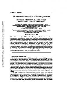
3. Numerical Simulation of PVDF Sensor’s Response to Impact Force Numerical simulation was conducted using MATLAB. The sampling rate was chosen as 10 kHz and one second of the PVDF sensor’s output voltage response was simulated. The basic input parameters for simulation are shown in Table 1. Figure 3 illustrates the simulation flow. Three vibration modes were included for impact at locations 1 and 2 and five modes for location 3. Natural frequencies of the cantilever beam were determined using Equations (9) and (16) for flexural modes. Damping ratios obtained by the half-power method (Table 3) were employed to create the unit impulse-response function. For mode shape simulation, the length increment of 1 mm was chosen. Impact time-histories at three impact locations illustrated in Figure 4 were employed as input impact loading in the simulation process (Figure 5). The unit impulse-response function, modal response, and mode shape slope difference are determined for each vibration mode. The electrical charge is then summed from the contribution of all included vibration modes. Predicted output voltage is finally determined from the electrical charge determined by Equation (20).
Impact time-histories at three impact locations illustrated in Figure 4 were employed as input impact loading in the simulation process (Figure 5). The unit impulse-response function, modal response, and mode shape slope difference are determined for each vibration mode. The electrical charge is then summed from the contribution of all included vibration modes. Predicted output voltage is Sensors 16, 601 7 of 15 finally2016, determined from the electrical charge determined by Equation (20).
Figure 3. Flow of numerical simulation.
Sensors 2016, 16, 601
8 of 14
Force [N]
Figure Configuration of Figure 4. 4. Configuration of cantilever cantilever beam beam with with attached attached sensor sensor and and impact impact locations locations (Unit: (Unit: mm). mm).
loadings at at three Figure 5. Time-histories of impact loadings three locations. locations.
5. Verification of Numerical Simulation Results by FEM In order to verify the simulation results, FE model of the cantilever beam subjected to impact loading was analyzed using the commercial software ABAQUS. The purposes of FEM analysis were: (1) To acquire the knowledge of the cantilever beam’s vibration modes, as well as mode shapes and natural frequencies that would be used for the numerical simulation; (2) to obtain dynamic strain for verification of the numerical simulation results; and (3) to convert output impact histories of the ICP signal conditioner into force unit. Table 2 indicates that the natural frequencies of the cantilever beam obtained by FEM analysis, classical beam theory, and modal impact test exhibit a good agreement. Most of the flexural modes can be accurately identified by the PVDF sensor, which
Sensors 2016, 16, 601
8 of 15
Table 1. Input parameters for simulation. Item
Symbol
Parameter
Value
Sensor
Lp bp tp d31 Ep Cp
Length Width Thickness Piezoelectric constant Young’s modulus Capacitance
155 mm 19 mm 0.028 mm 23 ˆ 10´12 (C/N) 4 GPa 11 nF
Charge Amplifier
fc CF
Cut-off frequency Feedback capacitance
0.1 Hz 100 nF
Cantilever beam
ρ E
Density Young’s modulus
7860 kg/m3 200 GPa
4. Impact Tests To obtain the actual impact histories that would be input for numerical simulation and to verify the numerical simulation results, impact tests were conducted by applying impact loadings on a steel cantilever beam on which a PVDF sensor was attached. The piezofilm lab amplifier [34] operating in charge mode was used for signal conditioning. Feedback capacitance of 100 nF was selected. The lower cut-off frequency and higher cut-off frequency were selected as 0.1 Hz and 100 kHz, respectively. The NI USB-4431 enabling four 24-bit simultaneous analog inputs was used for data acquisition. 10 kS/s was chosen for sampling rate and 1 kS/s for data windowing for real-time visualization of the PVDF sensor’s output response during the impact tests. One DT4-028 K/L PVDF sensor [35] was attached to the steel cantilever beam by a commercial double-coated adhesive tape. One edge of the PVDF sensor distances 30 mm from the fixed end of the cantilever beam (Figure 4). The impact hammer PCB 086C03 manufactured by PCB Piezotronics with a mounted plastic tip was used to apply impact force on the cantilever beam at the three impact locations illustrated in Figure 4. During the impact tests, impact signal was transmitted to the ICP sensor signal conditioner provided by PCB Piezotronics. A unit gain was set on the ICP signal conditioner. To verify the numerical simulation results, strain gages were also attached to the opposite side of the cantilever beam to obtain “true” strain (Figure 4). Typical impact force time-histories are shown in Figure 5. Impact force histories at locations 1 and 2 contain two peaks which are both due to the physical contact between the impact hammer and the cantilever beam. Particularly, the first peak represents the first time when the cantilever beam is collided by the hammer tip. The energy absorbed by the cantilever beam is then transformed to displacement of the cantilever beam’s free end, which mainly excites the first vibration mode. Right after the first collision, the hammer tip continues to move in the same direction as that of the cantilever beam’s free end due to the effect of inertia induced by the hammer’s weight and velocity. Approximately one to two milliseconds after the first collision, the hammer hits the tip of cantilever beam the second time, which causes the second impact. However, for impact at location 3 which is close to the fixed end, impact energy absorbed by the cantilever beam is transformed mainly into excitation of higher modes rather than displacement at the point of collision. Therefore, only one peak appears in the time history of impact at location 3. However, time history of impact rather than impact force magnitude (i.e., peak) was employed in the numerical simulation, which means impact force energy is taken into account in the prediction of the PVDF sensor’s output voltage in this study. 5. Verification of Numerical Simulation Results by FEM In order to verify the simulation results, FE model of the cantilever beam subjected to impact loading was analyzed using the commercial software ABAQUS. The purposes of FEM analysis were: (1) To acquire the knowledge of the cantilever beam’s vibration modes, as well as mode shapes and natural frequencies that would be used for the numerical simulation; (2) to obtain dynamic strain for verification of the numerical simulation results; and (3) to convert output impact histories of the ICP
Sensors 2016, 16, 601
9 of 15
signal conditioner into force unit. Table 2 indicates that the natural frequencies of the cantilever beam obtained by FEM analysis, classical beam theory, and modal impact test exhibit a good agreement. Most of the flexural modes can be accurately identified by the PVDF sensor, which indicates the capability of PVDF sensors in identifying natural frequencies of the host structure’s fundamental vibration modes. The first torsional mode at 341.41 Hz did not appear in the frequency response functions (Figure 6), which may indicate the dominance of flexural modes for all three impact locations. If torsional modes are excited due to an impact location that deviates from the central line of the cantilever beam, PVDF sensors can also capture such torsional modes. The superiority of PVDF sensors compared to conventional foil strain gages in capturing torsional modes was indicated in Ma et al. [26]. For the second purpose, FEM modal dynamic analysis was conducted using the actual recorded impact that had been previously generated by the impact hammer during the impact tests. Direct damping ratios (Table 3) determined by the half-power point method [36] using the frequencies response functions shown in Figure 6 were used for the first five flexural modes of the cantilever beam in the FEM analysis. To obtain the theoretically simulated strain shown in Figure 7, the transverse displacement in Equation (4) was determined from the mass-normalized eigenfunction written in Equation (5) and the modal coordinate (i.e., the solution of Equation (12)) expressed in Equation (15). Dynamic strain was then calculated in Equation (3) by taking the second derivative of the known transverse displacement. There appears to be a good agreement between the strain values obtained by FEM analysis, those measured in the impact tests and those predicted by the numerical simulation for impacts at locations 1 and 2 (Figure 7a,b). For impact at location 3, only the strain values determined by FEM analysis and those predicted by simulation were compared since the strain amplitude is only as low as the noise level in strain gages. A good agreement was also observed for impact location 3 (Figure 7c). Table 2. Natural frequencies of the cantilever beam (Hz). Modal Test Theory
Location 2
Location 3
Maximum Difference (%)
12.29
12.3
12.32
2.02
77.06
77.08
77.15
1.94
n/a
n/a
0.79
215.4
215.5
1.69
Mode Type
FEM
1
1st Flexural
12.135
12.071
2
2nd Flexural
76.029
75.651
3
1st Lateral
120.44
n/a
119.5
4
3rd Flexural
212.89
211.85
215.2
5
1st Torsional
341.41
n/a
n/a
n/a
n/a
n/a
6
4th Flexural
417.28
415.14
422.4
422.5
422.9
1.83
7
5th Flexural
690.06
686.19
698.3
698.3
698.9
1.81
8
2nd Lateral
739.77
n/a
n/a
n/a
n/a
n/a
9
2nd Torsional
1026.7
n/a
n/a
n/a
n/a
n/a
10
6th Flexural
1031.3
1025.1
1044
1044
1044
1.81
Mode No.
Location 1
Table 3. Idenfified damping ratio by half-power method.
Impact at 1 Impact at 2 Impact at 3
1st Mode
2nd Mode
3rd Mode
4th Mode
5th Mode
0.011159 0.009391 0.013542
0.002566 0.002647 0.002346
0.005434 0.006121 0.005920
0.001362
0.002831
Equation (12)) expressed in Equation (15). Dynamic strain was then calculated in Equation (3) by taking the second derivative of the known transverse displacement. There appears to be a good agreement between the strain values obtained by FEM analysis, those measured in the impact tests and those predicted by the numerical simulation for impacts at locations 1 and 2 (Figure 7a,b). For impact at location 3, only the strain values determined by FEM analysis and those predicted by Sensorssimulation 2016, 16, 601 10 of 15 were compared since the strain amplitude is only as low as the noise level in strain gages. A good agreement was also observed for impact location 3 (Figure 7c). 20 Location 1 Location 2 Location 3
0 -20 -40 -60
0
100
200
300
400
500
Frequency [Hz] Sensors 2016, 16, 601
10 of 14
Figure 6. Frequency response functions for three impact locations.
Figure 6. Frequency response functions for three impact locations. Table 2. Natural frequencies of the cantilever beam (Hz). 500
Mode No.
Mode Type
FEM
Theory
1 2 3 4 5 6 7 8 9 10
1st Flexural 2nd Flexural 1st Lateral 3rd Flexural 1st Torsional 4th Flexural 5th Flexural 2nd Lateral 2nd Torsional 6th Flexural
12.135 76.029 120.44 212.89 341.41 417.28 690.06 739.77 1026.7 1031.3
12.071 75.651 n/a 211.85 n/a 415.14 686.19 n/a n/a 1025.1
Location 1 12.29 77.06 119.5 215.2 n/a 422.4 698.3 n/a n/a 1044
Modal Test Location 2 12.3 77.08 n/a 0 215.4 n/a 422.5 698.3 -500 n/a 0 n/a 1044
(a)
Maximum Difference (%) Location 3 12.32 2.02 77.15 1.94 n/a 0.79 215.5 1.69 n/a n/a FEM 422.9 1.83 Experiment Simulation 698.9 1.81 n/a n/a 0.1 n/a n/a Time [s] 1044 1.81
(b)
Table 3. Idenfified damping ratio by half-power method. 400
Impact at 1 Impact 200 at 2 Impact at 3 0
1st Mode 0.011159 0.009391 0.013542
2nd Mode 0.002566 0.002647 0.002346
-200
400 3rd Mode 0.005434 200 0.006121 0.005920 0
4th Mode 0.001362
5th Mode 0.002831
FEM Experiment Simulation
-200
-400
-400 0
0.1
0.2
0.3
0.4
0.5
Time [s]
0
0.1
Time [s]
(c)
(d)
FEM Simulation Experiment
50
0
-50
0
0.1
0.2
Time [s]
(e)
(f)
Figure 7. Strain measured at 70 mm from the fixed end for three impact locations. (a,b) Impact at
Figure 7. Strain measured at 70 mm from the fixed end for three impact locations. (a,b) Impact at location 1; (c,d) Impact at location 2; (e,f) Impact at location 3. location 1; (c,d) Impact at location 2; (e,f) Impact at location 3.
6. Results of Numerical Simulation There appears to be a good agreement between the actual output voltage of the PVDF sensor obtained in the impact test and that predicted by the numerical simulation. Even for impact at location 3 for which the amplitude of output signal is much lower than that for locations 1 and 2 (Figure 8a,b), a reasonable prediction by simulation was also obtained (Figure 8c,d).
Sensors 2016, 16, 601
11 of 15
6. Results of Numerical Simulation There appears to be a good agreement between the actual output voltage of the PVDF sensor obtained in the impact test and that predicted by the numerical simulation. Even for impact at location 3 for which the amplitude of output signal is much lower than that for locations 1 and 2 (Figure 8a,b), 2016, 16, 601 11 of 14 aSensors reasonable prediction by simulation was also obtained (Figure 8c,d). 0.6 Experiment Simulation
0.5
Experiment Simulation
0.4 0.2 0
0
-0.2 -0.5
-0.4 -0.6 0
0.1
0.2
0.3
0.4
0.5
0
Time [s]
0.1
0.2
0.3
0.4
0.5
Time [s]
(a)
(b) Experiment Simulation
0.03 0.02 0.01 0 -0.01 -0.02 0
0.05
Time [s]
(c)
(d)
Figure 8. Simulation results for three impact locations. (a) Impact at location 1; (b) Impact at Figure 8. Simulation results for three impact locations. (a) Impact at location 1; (b) Impact at location 2; location 2; (c,d) Impact at location 3. The sensor size is 155 × 19 × 0.028 (mm). One sensor edge is (c,d) Impact at location 3. The sensor size is 155 ˆ 19 ˆ 0.028 (mm). One sensor edge is placed 30 mm placed 30 mm from the fixed end of the cantilever beam so that the lead wire goes towards the from the fixed end of the cantilever beam so that the lead wire goes towards the fixed end. fixed end.
Parametric conducted using sensor sizesize andand sensor position as input parameters for Parametricstudies studieswere were conducted using sensor sensor position as input parameters the simulation described in thein previous sectionsection in order investigate the effect sensorof fornumerical the numerical simulation described the previous into order to investigate theofeffect size and sensor position on the output voltage of a PVDF sensor. The input impact forces, damping sensor size and sensor position on the output voltage of a PVDF sensor. The input impact forces, ratios and all remaining parameters chosen were similar to those used to forthose the prediction of damping ratios and allinput remaining input were parameters chosen similar used for the output voltage shown in Figureshown 8. Fiveindifferent including 20, 40, 80, 160, and20, 24040, mm prediction of output voltage Figure sensor 8. Five lengths different sensor lengths including 80, were employed in the simulation. The width of simulated sensors is 20 mm. For the investigation 160, and 240 mm were employed in the simulation. The width of simulated sensors is 20 mm. Foron the the effect of sensor position, a midpoint positiona increment 10 mmincrement was used.of Figure 9 shows the investigation on the effect of sensor position, midpoint of position 10 mm was used. simulated output voltage for different sensor sizes and midpoint positions. For impact at location 1, Figure 9 shows the simulated output voltage for different sensor sizes and midpoint positions. For there appears to be one position at about 260 mm from the fixed end where the output voltage reaches impact at location 1, there appears to be one position at about 260 mm from the fixed end where the minimum regardless of sensor size.regardless PVDF sensors located the fixed end closer tend totogenerate output voltage reaches minimum of sensor size.closer PVDFto sensors located the fixed higher peak voltage, which may be attributed to the fact that in the first mode of vibration bending end tend to generate higher peak voltage, which may be attributed to the fact that in the first mode moment increases towards the fixed end. The fact that minimum occurs at about 260 mm of vibration bending moment increases towards the the fixed end. Thevoltage fact that the minimum voltage might be due to the problem of cancelling of mode shape slope calculated at the two opposite edges occurs at about 260 mm might be due to the problem of cancelling of mode shape slope calculated at ofthe PVDF (Equation For impact locations 2(22)). and 3, theimpact minimum output voltage twosensor opposite edges (22)). of PVDF sensorat(Equation For at locations 2 andoccurs 3, the atminimum multiple output positions, which may be due to the cancellation problem at multiple nodal points as a voltage occurs at multiple positions, which may be due to the cancellation problem
at multiple nodal points as a result of higher number of excited vibration modes. The first five flexural mode shapes as well as the corresponding nodal points for each mode shape were illustrated in Figure 10. For all three impact locations, a larger sensor tends to generate higher output voltage and vice versa. For impact location 3, a sensor longer than 240 mm appears to result in no increase in output voltage. Furthermore, larger sensors appear to result in larger variation in the
Sensors 2016, 16, 601
12 of 15
result of higher number of excited vibration modes. The first five flexural mode shapes as well as the corresponding nodal points for each mode shape were illustrated in Figure 10. For all three impact locations, a larger sensor tends to generate higher output voltage and vice versa. For impact location 3, a sensor longer than 240 mm appears to result in no increase in output voltage. Furthermore, larger sensors appear to result in larger variation in the output voltage, which means that the effect of sensor Sensors 2016, 16, 601 12 of 14 Sensors 2016, 16, 601 12 of 14 location tends to be more significant for sensor with larger sizes. 1.2
Max. Voltage [V] Max. Voltage [V]
1 0.8 0.6 0.4 0.2 0
1.2
20 mm 20 mm 40 mm 40 mm 80 mm 80 mm 160 mm 160 mm 240 mm 240 mm
1 0.8 0.6 0.4 0.2 00
0
(a)(a)
100 100
200 200
300 300
Distance [mm] Distance [mm]
400 400
500 500
(b)(b) 0.06 0.06
20 mm 20 mm 40 mm 40 mm 80 mm 80 mm 160 mm 160 mm 240 mm 240 mm
0.05 0.05 0.04 0.04 0.03 0.03 0.02 0.02 0.01 0.01 0
00
0
100 200 300 400 500 100 200 300 400 500
Distance [mm] Distance [mm]
(c) (c) Figure 9. Simulated output voltage of PVDF sensor with different sensor lengths andand positions. Figure 9. Simulated Figure 9. Simulated output output voltage voltage of of PVDF PVDF sensor sensor with with different different sensor sensor lengths lengths and positions. positions. (a) (a) Impact at location 1; (b) Impact at location 2; (c) Impact at location 3. 3. Impact at location 1; (b) Impact at location 2; (c) Impact at location (a) Impact at location 1; (b) Impact at location 2; (c) Impact at location 3.
Nodal point Nodal point
Figure Mode shapes of the first flexural vibration modes. Figure 10.10. Mode shapes of the first fivefive flexural vibration modes. Figure 10. Mode shapes of the first five flexural vibration modes.
7. Conclusions 7. Conclusions This study investigates thethe “stress-averaging” mechanism of of thethe in-plane sensing mode of of thethe This study investigates “stress-averaging” mechanism in-plane sensing mode PVDF sensor for dynamic strain sensing. A numerical simulation was conducted to predict the PVDF sensor for dynamic strain sensing. A numerical simulation was conducted to predict the output voltage response of of a PVDF sensor attached to to a steel cantilever beam subjected to to impact output voltage response a PVDF sensor attached a steel cantilever beam subjected impact
Sensors 2016, 16, 601
13 of 15
7. Conclusions This study investigates the “stress-averaging” mechanism of the in-plane sensing mode of the PVDF sensor for dynamic strain sensing. A numerical simulation was conducted to predict the output voltage response of a PVDF sensor attached to a steel cantilever beam subjected to impact loading based on the fundamental knowledge of piezoelectricity, classical beam theory, and signal conditioning. FEM analysis and impact tests were also conducted to verify the simulation results. The results of impact test indicate the excellent capability of PVDF sensors in capturing the fundamental natural frequencies of the cantilever beam. The PVDF sensor’s output voltage could be reasonably predicted by the numerical simulation. Parametric studies on the effects of sensor size and sensor position indicate that a larger sensor tends to generate higher output voltage and vice versa. Furthermore, the effect of sensor position seems to be more significant for larger sensors. However, when a large number of modes are excited, e.g., impact at location 3, increasing sensor size may not always result in increased output voltage. The sensor size beyond which increasing sensor size does not result in increased output voltage may depend on the number of dominant vibration modes which in turn depends on impact location. The results indicate that, in order to maximize the signal-to-noise ratio for actual measurements in small scale structures (i.e., the size of an attached PVDF sensor is relatively large with respect to the size of the host structural member), vibration mode shapes of the structural member should be considered to choose the optimal sensor location that helps avoid the cancelling problem. Overall, PVDF sensors exhibit an excellent in-plane sensing capability for dynamic strain induced by impact loading. Author Contributions: Both authors conceived and designed the experiments; the first author performed the experiment, analyzed the data, proposed the numerical simulation, and wrote the paper. The second author dedicated his valuable suggestions and comments on the interpretation of results and on the paper. Conflicts of Interest: The authors declare no conflict of interest.
References 1. 2. 3. 4. 5. 6. 7. 8. 9. 10.
11.
12.
Kawai, H. The piezoelectricity of poly (vinylidene fluoride). Jpn. J. Appl. Phys. 1969, 8, 975–976. [CrossRef] Lando, J.B.; Olf, H.G.; Peterlin, A. Nuclear magnetic resonance and x-ray determination of the structure of poly (vinylidene fluoride). J. Polym. Sci. 1966, 4, 941–951. [CrossRef] Sessler, G.M. Piezoelectricity in polyvinylidenefluoride. J. Acoust. Soc. Am. 1981, 70, 1596–1608. [CrossRef] Darasawa, N.; Goddard, W.A. Force fields, structures, and properties of poly (vinylidene fluoride) crystals. Macromolecules 1992, 25, 7268–7281. Lee, L.M.; Graham, R.A.; Bauer, F.; Reed, R.P. Standardized Bauer PVDF piezoelectric polymer shock gauge. J. De Physique 1988, 9, 651–657. [CrossRef] Dutta, P.K.; Kalafut, J. Evaluation of PVDF Piezopolymer for Use as a Shock Gauge; Special Report; U.S. Army Corps of Engineers: Hanover, NH, USA, 1990; pp. 90–23. Bauer, F. Ferroelectric PVDF polymer for high pressure and shock compression sensors. In Proceedings of the 11th International Symposium on Electrets, Melbourne, Australia, 1–3 October 2002; pp. 219–222. Shirinov, A.V.; Schomburg, W.K. Pressure sensor from a PVDF film. Sens. Actuators A 2008, 142, 48–55. [CrossRef] Wang, F.; Tanaka, M.; Chonan, S. Development of a wearable mental stress evaluation system using PVDF sensor. J. Adv. Sci. 2006, 18, 170–173. [CrossRef] Kim, K.J.; Chang, Y.M.; Yoon, S.; Kim, H.J. A Novel Piezoelectric PVDF Film-Based Physiological Sensing Belt for a Complementary Respiration and Heartbeat Monitoring System. Integr. Ferroelectr. 2009, 107, 53–68. [CrossRef] Chiu, Y.; Lin, W.; Wang, H.; Huang, S.; Wu, H. Development of a piezoelectric polyvinylidene fluoride (PVDF) polymer-based sensor patch for simultaneous heartbeat and respiration monitoring. Sens. Actuators A 2013, 189, 328–334. [CrossRef] Woodward, B.; Chandra, R.C. Underwater acoustic measurements on polyvinylidene fluoride transducers. Electrocomponent Sci. Technol. 1978, 5, 149–157. [CrossRef]
Sensors 2016, 16, 601
13. 14.
15. 16. 17. 18. 19.
20. 21.
22. 23. 24. 25. 26. 27. 28. 29. 30. 31. 32. 33. 34.
14 of 15
Xu, J. Microphone Based on Polyvinylidene Fluoride (PVDF) Micro-Pillars and Patterned Electrodes. Ph.D. Thesis, Ohio State University, Columbus, OH, USA, 2010. Headings, L.M.; Kotian, K.; Dapino, M.J. Speed of sound measurement in solids using polyvinylidene fluoride (PVDF) sensors. In Proceedings of the ASME 2013 Conference on Smart Materials, Adaptive Structures and Intelligent Systems, SMASIS2013, Snowbird, UT, USA, 16–18 September 2013. Xu, J.; Headings, L.M.; Dapino, M.J. High sensitivity polyvinylidene fluoride microphone based on area ratio amplification and minimal capacitance. IEEE Sens. J. 2015, 15, 2839–2847. [CrossRef] Lee, M.H.; Nicholls, H.R. Tactile sensing for mechatronics—A state of the art survey. Mechatronics 1999, 9, 1–31. [CrossRef] Dargahi, J. A piezoelectric tactile sensor with three sensing elements for robotic, endoscopic and prosthetic applications. Sens. Actuators A 2000, 80, 23–30. [CrossRef] Seminara, L.; Capurro, M.; Cirill, P.; Cannata, G.; Valle, M. Electromechanical characterization of piezoelectric PVDF polymer films for tactile sensors in robotics applications. Sens. Actuators A 2011, 169, 49–58. [CrossRef] Ma, C.; Chuang, K.; Pan, S. Polyvinylidene Fluoride Film Sensors in Collocated Feedback Structural Control: Application for Suppressing Impact-Induced Disturbances. IEEE Trans. Ultrason. Ferroelectr. Freq. Control 2011, 12, 2539–2554. [CrossRef] [PubMed] Matsumoto, E.; Biwa, S.; Katsumi, K.; Omoto, Y.; Iguchi, K.; Shibata, T. Surface strain sensing with polymer piezoelectric film. NDT&E Int. 2004, 37, 57–64. Kurata, M.; Li, X.; Fujita, K.; He, L.; Yamaguchi, M. PVDF Piezo Film as Dynamic Strain Sensor for Local Damage Detection of Steel Frame Buildings. In Proceedings of the SPIE Sensors and Smart Structures Technologies for Civil, Mechanical, and Aerospace Systems, San Diego, CA, USA, 10 March 2013. Bloomfield, P.E. Piezoelectric Polymer Transducers for Detection of Structural Defects in Aircraft; Final Report; Naval Air Development Center: Warminster, PA, USA, 1977. Lee, C.K.; O’Sullivan, T.C. Piezoelectric strain rate gages. J. Acoust. Soc. Am. 1991, 2, 945–953. [CrossRef] Wang, B.; Wang, C. Feasibility analysis of using piezoceramic transducers for cantilever beam modal testing. Smart Mater. Struct. 1997, 6, 106–116. [CrossRef] Sirohi, J.; Chopra, I. Fundamental Understanding of Piezoelectric Strain Sensors. J. Intell. Mater. Syst. Struct 2000, 11, 246–257. [CrossRef] Ma, C.; Huang, Y.; Pan, S. Investigation of the Transient Behavior of a Cantilever Beam Using PVDF Sensors. Sensors 2012, 12, 2088–2117. [CrossRef] [PubMed] Kotian, K.; Headings, L.M.; Dapino, M.J. Stress Averaging in PVDF Sensors for in-Plane Sinusoidal and Impact-Induced Stresses. IEEE Sens. J. 2013, 11, 4444–4451. [CrossRef] Standards Committee of IEEE Ultrasonics. Ferroelectrics, and Frequency Control Society; IEEE Standard on Piezoelectricity: New York, NY, USA, 1987. Beer, F.P.; Johnston, E.R.; Dewolf, J.T. Mechanics of materials, 5th ed.; McGraw-Hill Inc.: New York, NY, USA, 2006. Caughey, T.K.; O’Kelly, M.E.J. Classical Normal Modes in Damped Linear Dynamic Systems. ASME J. Appl. Mech. 1965, 32, 583–588. [CrossRef] Erturk, A.; Inman, D.J. A Distributed Parameter Electromechanical Model for Cantilevered Piezoelectric Energy Harvesters. J. Vib. Acoust. 2008, 130, 1–15. [CrossRef] Erturk, A. Electromechanical Modeling of Piezoelectric Energy Harvesters. Ph.D. Thesis, Virginia Polytechnic Institute and State University, Blacksburg, VA, USA, 2008. Measurement Specialties Inc. Piezo Film Sensors Technical Manual. Available online: http://www. meas-spec.com/downloads/Piezo_Technical_Manual.pdf (accessed on 7 July 2015). Measurement Specialties Inc. Piezo Film Lab Amplifier. Available online: http://www.meas-spec.com/ downloads/Piezo_Film_Lab_Amplifier.pdf (accessed on 25 March 2015).
Sensors 2016, 16, 601
35. 36.
15 of 15
Measurement Specialties Inc. DT Series Elements with Lead Attachment. Available online: http://www.meas-spec.com/downloads/DT_Series_LeadAttach.pdf (accessed on 5 March 2015). Butterworth, J.; Lee, J.H.; Davidson, B. Experimental determination of modal damping from full-scale testing. In Proceedings of the 13th World Conference on Earthquake Engineering, Vancouver, BC, Canada, 1–6 August 2004. © 2016 by the authors; licensee MDPI, Basel, Switzerland. This article is an open access article distributed under the terms and conditions of the Creative Commons Attribution (CC-BY) license (http://creativecommons.org/licenses/by/4.0/).