Debris-Covered Glaciers (Proceedings of a workshop held at Seattle, Washington, USA, September 2000). IAHS Publ. no. 264, 2000.
245
Numerical simulation of recent shrinkage of Khumbu Glacier, Nepal Himalayas
NOZOMU NAITO, MASAYOSHI NAKAWO Institute for Hydrospheric-Atmospheric Nagoya 464-8601, Japan
Sciences, Nagoya University, Furo-cho,
Chikusa-ku,
e-mail:
[email protected],jp
TSUTOMU KADOTA Frontier Observational Research System for Global Change, Sumitomo Hamamatsu-cho Building 4F, 1-8-16 Hamamatsu-cho, Minato-ku, Tokyo 105-0013, Japan
CHARLES F. RAYMOND Geophysics Program, University of Washington, Box 351650, Seattle, Washington USA
98195-1650,
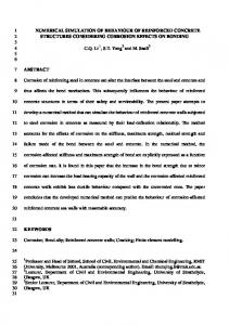
Abstract A new model for coupled mass balance and flow of a debris-covered glacier was developed to account for the effects of supraglacial debris on glacier evolution. The model is reasonably consistent with observations of recent shrinkage of the ablation area of Khumbu Glacier, Nepal Himalayas from 1978 to 1999. The model predicts formation and succeeding enlargement of a depression in the lower ablation area. This depression could result in the formation of a glacial lake. Potential improvements to the model for a debriscovered glacier are identified. INTRODUCTION The ablation areas of most large glaciers in the Himalayas are covered with thick supraglacial debris. It is, hence, important to know how these debris-covered glaciers in the Himalayas respond to climate change in order to predict consequences for local water resources and sea level rise. Khumbu Glacier is one of the largest debris-covered glaciers in the Nepal Himalayas. It flows down from the slopes of Mts Everest (8848 m, Sagarmatha or Qomolangma), Lhotse (8511 m) and Nuptse (7861 m) (Fig. 1). Its total length is more than 15 km and its present terminus is located at about 4900 m a.s.l. The accumulation area, called the West Cwm, is nearly inaccessible due to an ice fall. The equilibrium line altitude (ELA) is located in this ice fall at about 5600 m a.s.l. More glaciological research has been undertaken on the ablation area than on any other debris-covered glacier in the Himalayas. Recent thinning of the glacier has been measured (Kadota et al., 2000). This study establishes a new numerical model to simulate the recent shrinkage of the glacier accounting for supraglacial debris and its effects on ablation. MODEL DESCRIPTION The continuity equation coupling mass balance and glacier flow was formulated using the finite-volume method (Patankar, 1980; Lam & Dowdeswell, 1996):
246
Nozomo
Naito et al.
x
F i g . 1 Illustrated m a p of K h u m b u Glacier. T h e study area is a l o n g a central flow line indicated as a d a s h e d line with an arrow.
where V, b, W and Q represent volume between fixed vertical cross-sections, mass balance rate, glacier surface width averaged between the sections, flux through the boundary cross-section to/from neighbouring control-volumes, respectively. Subscripts for Q refer to outgoing or incoming flux, t and x are time and horizontal distance along a flow line traced in Fig. 1. Time step, At, was 1/36 year (about 10 days), and the longi tudinal length of each control-volume (grid space), Ax, was 500 m. Equation (1) was stepped forward in time using an implicit Crank-Nicholson scheme with calculations of mass balance and glacier flow described in the following subsections. The simulation, however, was limited to the ablation area with an assumption about flux through the upper boundary cross-section, which will be described later. A trapezoidal cross-section was assumed for the glacier channel with lateral slopes of 40° and 35° for the right and left bank sides, respectively, as compatible with a topographic survey by Glaciological Expedition of Nepal (1980). Glacier width was approximated with a linear variation to fit measurements from the topographic map published by the National Geographic Society (1988). The profile of the glacier bed was determined by ice thickness measure ments with ice penetrating radar (Gades et ai, 2000) and topographic surveys in 1999. Mass balance Glaciers in the Himalayas are fed mostly in summer, and this summer-accumulationtype mass balance has to be taken into consideration. Empirical equations among air temperature T (°C), precipitation rate P (m day" ), accumulation rate c (m day" ) and ablation rate a (m day" ) were obtained for a debris-free glacier in the Nepal Himalayas by Ageta (1983) and Ageta & Kadota (1992) as follows: 1
1
1
Numerical
C
simulation
of recent shrinkage
of Khumbu
Glacier,
=P
when T < -0.6
= P ( 0 . 8 5 - 0.247/)
when -0.6 3.5
a =0
Nepal
247
Himalayas
when T< -3.0 ,3.2
= -0.0001(7+3.0)-
when -3.0 2.0
(2)
Seasonal variations in P and T were approximated by sinusoidal variations, having the same phase (i.e. high/low in summer/winter). Annual mean air temperature was set to be compatible with a measurement in 1973-1974 at Lhajung (0.5°C at 4420 m a.s.l.) (Inoue, 1976), accounting for a fixed altitudinal lapse rate of - 6 x 10" °C m" . Annual range of air temperature and annual precipitation were assumed to be the same as at Lhajung (15°C and 540 mm, respectively) and independent of altitude. Lhajung is located at about 5 km southeast of the Khumbu Glacier terminus. Effects of debris cover on the ablation have been examined in the following ways. Nakawo et al. (1999) estimated the longitudinal distribution of the ablation rate for the whole ablation area, using satellite data and meteorological data. As accumulation to the glacier ice body is • negligible on the debris-covered ablation area, the estimated ablation rate was taken to be equivalent to the mass balance rate. They, however, implied that the magnitude of the mass balance rate may be in error due to uncertainty in meteorological data input. Surface lowering rate calculated by the continuity equation with observed surface flow speed was compared with that measured by Kadota et al. (2000). The comparison indicated that the calculated surface lowering rate was larger than the measurement on the lowest part of the glacier. The longitudinal distribution of mass balance rate, therefore, was slightly modified from the estimate by Nakawo et al. (1999) as shown in Fig. 2(a). A hypothetical mass balance rate for debris-free conditions is also shown in Fig. 2(a), which was calculated with equation (2) with the distribution and the seasonal variation of air temperature based on the surface altitude from the topographic surveys in 1978 (Watanabe et al, 1980). The ratio r of the mass balance for debriscovered conditions to that for debris-free conditions was evaluated from the solid and dashed curves in Fig. 2(a). The longitudinal distribution of debris thickness H was measured by Nakawo et al. (1986) and Watanabe et al. (1986). The implied relationship between r and H is shown in Fig. 2(b). As a result, net ablation (negative mass balance) on the debris-covered area can be calculated from c, a in equation (2) and r which depends on H (Fig. 2(b)). However, special attention must be given to the situation when supraglacial debris is covered with snow. If debris cover is buried by snow cover, water equivalent thickness of the snow cover H varies depending on c + a in equation (2), and the mass of glacier ice beneath the debris cover does not change. There is no melt-out debris supply from glacier ice in this case. If net ablation exceeds an amount required to melt all the snow cover, however, extra ablation of glacier ice occurs according to the residual amount of net ablation, (c + a)Ar + H ( 0 md (c + a)At + H < 0
=0
when H >0
s
d
s
d
and (c + a)At + H >0 S
(3)
Water equivalent thickness of snow cover H varies as: s
AH s
- =c +a
when H > 0 and (c + a)At + H >0 d
S
At H =0
in the other cases
s
(4)
Debris thickness H varies according to the continuity equation for supraglacial debris: d
D
D
= £jL( y o^~ in p
when b < 0
rb
At
WAx
d
£> - A . out
WAx
in
when b > 0
(5)
Numerical
simulation
of recent shrinkage
of Khumbu
Glacier, Nepal
Himalayas
249
where Cd, pd and D are concentration of debris in glacier ice, density of debris, and flux of supraglacial debris through a boundary between neighbouring control-volume, respectively. The concentration of debris Q and the density were assumed to be constants 0.1 kg nf and 1220 kg m" (Nakawo et al, 1986), respectively. Subscripts for D refer to outgoing or incoming flux. The flux D is described as: 3
3
D = H WU,
(6)
d
where U is surface flow speed, which is described by equation (7) in the next subsection. Note, here, each variable on the right side in equation (6) should be that at the boundary between control-volumes. s
Glacier flow Surface flow speed U and flux of glacier ice through a cross-section Q can be described as: s
U,=U U J+
(7)
b
Q = (f U +U )S 2
d
(8)
b
+l
U =^-(-f mayH" d
(9)
lPgS
n +l
Ud is a contribution of ice deformation to the surface flow speed. lf represents a basal sliding. A and n (= 3) are parameters in the flow law of ice; p and g are the density of ice and the gravitational acceleration; a, H and S are the surface slope, the central ice thickness and the transversal cross-section area, respectively. fa and fa are so-called "shape factors", which account for lateral drag in equation (9) and ratio of crosssectional average ice deformation to Ud in equation (8). The value of A was assumed to be constant, 6.8 x 10" s" (kPa)" , which is a recommended value for ice temperature of 0°C by Paterson (1994). The value of the shape factor fa was approximated with b
15
W/1H
3
W/2H
033 +0J8 2
1
1
( 1 Q )
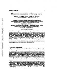
which fits with the values obtained by Nye (1965) for a parabolic cross-section, as the value of/i should not be so different from that for a trapezoidal cross-section, which was used in this model. The flow speed ratio fa was assumed to be the same as for laminar flow, n + 1/n + 2 (= 0.8), which neglects variation in flow speed ratio across the flow. Then U was assumed to be distributed in the ablation area independent of time as shown in Fig. 3, which gives surface flow speed U consistent with observation (Kodama & Mae, 1976; Nakawo et al, 1999). Inflow from the upper glacier area 2,„(x= 0) was assumed to be constant as 5.6 x 10 kg year" . This value yields agreement between modelled and observed (Kadota et al, 2000) surface lowering at x = 0, and is about 1.5 times that of an earlier rough estimate by Inoue (1977), which was based on the assumptions that precipitation on the accumulation area would be the same as at Lhajung independent of altitude and that the accumulation area was in a steady state. 0
s
9
1
250
Nozomo
Naito et al.
60
CL CO
S 2 0 4-
o Œ
K4 o 0
2000
4000
8t 0 0 0
6000
10000
Longitudinal distance (m) F i g . 3 F l o w speeds on the K h u m b u Glacier. S q u a r e and plus s y m b o l s are the o b s e r v e d surface speeds b y K o d a m a & M a e (1976) in 1 9 7 3 - 1 9 7 4 and N a k a w o et al. (1999) in 1 9 8 7 - 1 9 9 3 , respectively. T h e solid c u r v e represents the calculated surface speed b a s e d o n the surveyed profile in 1978, and the d a s h e d c u r v e s h o w s that b a s e d o n a profile in 1990 estimated from topographic surveys in 1978 and 1999. D o t t e d curve is basal sliding JJ a s s u m e d in this study to tune the calculated surface speeds to the observations. b
RESULTS OF SIMULATION The initial conditions were the longitudinal profiles in 1978 of surface elevation (Watanabe et al., 1980) and supraglacial debris thickness (Nakawo et al., 1986; Watanabe et al., 1986). Climate was assumed to be constant as in 1973-1974 (Inoue, 1976), since there are no available data about climate changes around the Khumbu Glacier. Furthermore, Kadota & Ageta (1992) succeeded in simulating shrinkage of a debris-free glacier near the Khumbu Glacier in 1978-1989 without significant climate change, which supports this assumption. Predictions for changes in surface elevation and debris thickness are shown in Fig. 4. The longitudinal surface profile in 1999 is simulated quite reasonably (Fig. 4(a)). The succeeding simulation predicts that a depression would be formed at about x = 5.5 km around year 2020 and the ablation area would be divided into two parts around year 2040. Debris thickness Hd is predicted to decrease on the uppermost part, to increase on the lowest part and near the predicted terminus after the glacier division (Fig. 4(b)).
Sensitivity tests Sensitivity tests for the simulation of the longitudinal surface profile were examined concerning three important parameters: incoming flux at the upper boundary, basal sliding, and the effect of debris on the mass balance. Figure 5 shows the simulated profiles for 1999 under three different conditions, together with the preceding result. Assuming the incoming flux Q (x = 0) = 3.8 x 10 kg year" to be the same as Inoue's (1977) earlier rough estimate, the simulated glacier surface lowering during 19781999 was predicted to be about twice as large as the observation on the uppermost part. On the other hand, neglecting basal sliding U resulted in almost the same surface 9
in
D
1
Numerical
simulation
of recent shrinkage
of Khumbu
Glacier,
Nepal
Himalayas
251
5400 j 5300 *'\ g 5200 -