Use may be made of the PHOENICS [1] mathematical simulation program. When the results are presented in tables, another mathematical simulation program is ...
Chemical and Petroleum Engineering, Vol. 39, Nos. 9–10, 2003
INDUSTRIAL ECOLOGY NUMERICAL SIMULATION OF SOLID PARTICLE PROPAGATION IN THE ATMOSPHERE
P. Baltrenas, S. Vasarevicius, and E. Petraitis
Numerical models are currently mainly used to estimate air pollution in Lithuania. For example, the VARSA program has been used to determine pollution standards for industry, but this model was developed by a method itself devised 20 years ago, which has a narrow sphere of application and many shortcomings. Therefore, numerical simulation of gas and heavy aerosol propagation remains a current problem. It is extremely difficult to obtain an exact analytic solution, so approximate methods are required. Use may be made of the PHOENICS [1] mathematical simulation program. When the results are presented in tables, another mathematical simulation program is used: SURFER, which processes the results and presents them in visual form [2]. Calculation Model. Figure 1 shows the essential model for this case. It differs only slightly from the above programs. To illustrate the differences between VARSA and PHOENICS, we have taken heavy particles as representing the pollution. The pollution focus was a nominal power plant whose chimney has a height of 25 m, diameter of pollution source 25 m, and combustion product ejection speed 6 m/sec. The wind distributes the pollutant in a westerly direction with a speed of 2 m/sec, and the pollutant concentration at the discharge focus is C = 100 mg/m3. These parameters were used in both models. The size of the particles and the acceleration due to gravity were also introduced into the PHOENICS program [3]. The calculation net for VARSA was specified in the near-ground layer in a two-dimensional plane with the length, width, and step stated. In PHOENICS, we used a three-dimensional space, which was divided into calculation regions along the x, y, and z axes. In the SURFER package, the data may be represented in two-dimensional or three-dimensional planes [4]. Theoretical Assumptions. Dust and aerosol propagation is largely dependent on the physical and mechanical properties. For simulation it is very important to estimate them, particularly the processes occurring in the real medium. The VARSA program gives the maximum near-ground pollutant concentration as Cm =
AMFmnµ
,
(1)
H 2 3 V1∆T 4
where A is the vertical temperature lapse rate, M the pollutant discharge rate, F the deposited pollution coefficient, m and n are coefficients relating to the flux of the discharge from the source, H is the height of the pollutant source in m, µ the relief effect coefficient (µ = 1 when the height difference is up to 50 m at a distance of 1 km), ∆T is the temperature difference between the discharge and the atmosphere, and V1 is the gas discharge rate in m3/sec. The theoretical assumptions for this program have been dealt with fairly widely in the literature [5, 6]. Gediminas Vilnius Technical University. Translated from Khimicheskoe i Neftegazovoe Mashinostroenie, No. 10, pp. 46–48, October, 2003. 0009-2355/03/0910-0615$25.00 ©2003 Plenum Publishing Corporation
615
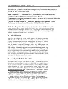
Fig. 1. Model scheme: 1) building; 2) chimney; 3) pollutant dispersal focus; 4) pollutant discharge; 5) working space.
H, m
Wind direction
C, mg/m3 Distance L, m
a
Distance L, m
b
Fig. 2. Particle propagation in the atmosphere provided by various pieces of software: a) VARSA; b) PHOENICS.
The PHOENICS program is one of the widely used computational fluid dynamics CFD programs, which solve the equations by finite-difference methods [7]. In that model, the elliptic equation system consists of equations for the momentum transported in three directions, the concentration, and continuity, as well as Newton’s law of viscosity, Fourier thermal conduction, and Fick diffusion. These equations can be written in the combined form [8]: ∂ r (r ρ Φ ) + div (riρi vΦ i − riΓi grad Φ i ) = ri S Φ , i ∂t i i i
(2)
where t is time, ri is the volume fraction of phase i (r = 1 in the single-phase case), ρi is the density of phase i, Φi is a variable associated with phase i (concentration, enthalpy, and so on), v is the velocity vector for phase i, Γi is a variable exchange coefficient, and SΦi represents the flux of variable Φi. Equation (2) is solved by finite-difference methods when the corresponding characteristic limiting conditions are given. The last is called the flux or source term and may have numerous and fairly complicated forms of expression. The main ones are intended for estimating the pressure gradient, Coriolis force, gravitation, and so on. One can select the necessary ones or introduce new ones. As the Coriolis force has only a small effect on the results, it needs to be estimated only in calculating global transfers, when part of the pollution is transported into the working medium from outside and substantially influences the results. The first term in the equation is not necessary when one examines stationary transport processes. 616
H, m
C, mg/m3 Distance L, m
Fig. 3. Particle distribution in the atmosphere calculated from the PHOENICS package.
C, mg/m3 C, mg/m3
a
b
Fig. 4. Particle distribution in the atmosphere given by the SURFER program: a) in two-dimensional space; b) in three-dimensional space.
The following formula was used in this case to calculate the particle flux and propagation: C=
(
)
24 0.42 1 + 0.15 Re 0.687 + , Re 1 + 4.25 ⋅ 25 ⋅ 10 4 Re −1.16
(3)
where Re is the Reynolds number. Particle propagation in the atmosphere has been calculated on the basis of the above assumptions [9]. Result Analysis. Figure 2a shows the highest concentrations of particles in the atmosphere at a distance L from the source as calculated from the VARSA program, where the maximal calculated concentration along the wind direction was 0.3 mg/m3. The VARSA program allows one to calculate the maximum permissible concentration only in a single horizontal plane and does not allow one to calculate the effects of time on any concentration fluctuations. For comparison, Fig. 2b shows the particle propagation in the atmosphere at 10 min after the operation of the source as calculated from the PHOENICS package. This package enables one to estimate particle propagation in relation to pollutant source height. If we take a slice below the chimney, we see that the particle concentration is reduced, the propagation width is altered somewhat, and the 617
image is obtained curved and does not give an exact representation of the particle propagation. The PHOENICS package enables one to use a calculation step by incorporating the time and gives a more accurate picture, i.e., it gives the concentrations not only in the ground layer but also at other levels, as well as in a vertical section. Figure 3 shows a vertical section of the particle pattern in the atmosphere after the source has been working for 10 min. The VARSA package does not allow one to do this [6]. The pollutant propagation pattern enables one to evaluate not only the vertical propagation but also the dependence of the pollutant concentration on the height of the focus. The PHOENICS package shows that the highest concentration lies around the focus, and if the source works continuously, almost the same concentration is formed in the ground layer. The concentration decreases away from the source, but the degree of influence from the pollutant increases. A few particles are deposited at a distance of about 50 m from the focus after the source has been operating for 10 min. The vertical propagation shows that the plume with the highest concentration rises to a height of up to 30 m. Figure 2b shows that the largest amount of pollutant is borne by the wind, and the propagation in the opposite direction from the source is slight (about 15 m). It is therefore very important to know the predominant wind directions in the locality, as this enables one to calculate the affected zones for the factory. Both of these programs have been set up to simulate pollutant propagation, but they do not allow one to operate with the available data. The SURFER package enables one to represent the calculations or measurements in two-dimensional or three-dimensional space, which facilitates visualizing the data. The representation model is chosen to suit the data type. In this particular case, the data are best represented in a plane (Fig. 4a) and in a spatial image (Fig. 4b), which clearly shows the maximum in the concentrations and the place where they occur. An advantage of the SURFER package is that one can vary the results and adjust the graphical representation, which in turn provides models for pollutant distribution as affected by any changes in the data over time or in response to other factors.
REFERENCES 1. 2. 3. 4. 5. 6. 7. 8.
9.
618
P. Baltrenas, A. Bakas, and R. Masilevicius, “Experimental investigation of electrostatic fabric filtration of wood fumes,” APLINKOS INZINERIJA, Technika, Vilnius, IX, No. 3, 170–175 (2001). R. Weinberger, “Entstauben von Rauschgasen: Technologien und deren Anwendung zur Entstaubung von Kesselanlagen,” Holz und Kunststoffverarb., Leipzig, No. 6, 52–53 (1997). P. Baltrenas, P. Vaitiekunas, and R. Vaiskunaite, “Numerical modeling of aerodynamic processes in a biofilter,” APLINKOS INZINERIJA (Environmental Engineering), Technika, Vilnius, IX, No. 4, 206–210 (2001). V. Kondrashov, A. Oznobishin, and V. Spakauskas, “Fuel injection system optimization by numerical experiments for reducing emissions into the atmosphere,” Technika, Vilnius, VII, No. 1, 10–14 (1999). Methods of Calculating Pollutant Concentrations in Atmospheric Air as Present in Factory Discharges: OND-86 [in Russian], Gidrometeoizdat, Leningrad (1987). H. I. Rosten and D. B. Spalding, Shareware PHOENICS: Beginner’s Guide, CHAM TR 1000, CHAM Ltd, London (1987). K.-D. Frohner and Th. Schulze, “Particle size sampling standards for airborne particles and experience with a personal online monitored particle-size sampling instrument,” Technika, Vilnius, VIII, No. 3, 110–115 (2000). P. Baltrenas, S. Vasarevicius, and E. Petraitis, “Numerical modelling of solid waste dispersion in the atmosphere using programs VARSA and PHOENICS,” APLINKOS INZINERIJA (Environmental Engineering), Technika, Vilnius, X, No. 1, 9–14 (2002). V. Makareviciene, S. Pukalskas, and P. Janulis, “Comparative investigation of rapeseed oil ethyl and methyl ester emissions,” APLINKOS INZINERIJA (Environmental Engineering), Technika, Vilnius, IX, No. 3, 158–163 (2001).