Numerical simulation of unsteady cavitation in liquid

Int. J. Engineering Systems Modelling and Simulation, Vol. 9, No. 1, 2017

41

Numerical simulation of unsteady cavitation in liquid hydrogen flows Eric Goncalvès ENSMA – Pprime, UPR 3346 CNRS, Poitiers, France Email: [email protected]

Dia Zeidan* School of Basic Sciences and Humanities, German Jordanian University, Amman, Jordan Email: [email protected] *Corresponding author Abstract: An unsteady cavitation model in liquid hydrogen flow is studied in the context of compressible, two-phase, one-fluid inviscid solver. This is accomplished by applying three conservation laws for mixture mass, mixture momentum and total energy along with gas volume fraction transport equation, with thermodynamic effects. Various mass transfers between phases are utilised to study the process under consideration. A numerical procedure is presented for the simulation of cavitation due to rarefaction and shock waves. Attention is focused on cavitation in which the simulated fluid is liquid hydrogen in cryogenic conditions. Numerical results are in close agreement with theoretical solutions for several test cases. The current numerical results show that liquid hydrogen flow can be accurately modelled using an accurate inviscid approach to describe the features of thermodynamic effects on cavitation. Keywords: two-phase flow; heat and mass transfer; liquid and hydrogen; homogeneous model; cavitation; splitting techniques; inviscid simulation. Reference to this paper should be made as follows: Goncalvès, E. and Zeidan, D. (2017) ‘Numerical simulation of unsteady cavitation in liquid hydrogen flows’, Int. J. Engineering Systems Modelling and Simulation, Vol. 9, No. 1, pp.41–52. Biographical notes: Eric Goncalvès is a Professor in the Aeronautical Engineering School ISAE-ENSMA, Poitiers, France. Currently, he is the Head of the Department Fluid Mechanics and Aerodynamics. His research interests are related to the modelling and the simulation of flows for which the density is variable such as compressible flow, two-phase flow and cavitation. Recent work include shock wave boundary layer interaction, thermal effects in cavitation and investigation of three-dimensional effects on cavitation pocket. Dia Zeidan is currently an Associate Professor in the School of Basic Sciences and Humanities at the German Jordanian University, Amman, Jordan. His expertise is in the mathematical modelling and numerical simulations of multiphase fluid flow problems. His recent work also includes hyperbolicity and conservativity resolution related to two-phase flows equations in the context of the Riemann problem and simulations of such flows over a wide range of non-equilibrium behaviours. This paper is a revised and expanded version of a paper entitled ‘Numerical study of cavitation in liquid hydrogen flow’ presented at 8th International Conference on Thermal Engineering Theory and Applications – ICTEA 2015, Amman, Jordan, 18–21 May 2015.

1 Introduction Thermodynamics of thermosensitive fluids is an essential phenomenon of cavitation dynamics arising in cryogenic fluids. These fluids are typically characterised by variations in fluid properties such as the temperature, with special Copyright © 2017 Inderscience Enterprises Ltd.

intense to vapour pressure. In cryogenic fluids, however, the density ratio of liquid-vapour is lower than the density of typical fluids such as cold water which leads to vapourisation of liquid mass to sustain a cavity. The evaporative cooling effects are more evident where the temperature of the liquid phase near the liquid-vapour

42

E. Goncalvès and D. Zeidan

interface is depressed below the free-stream temperature. Although the temperature depression is negligible in cold water, it remains a continuing interest in cavitation. Indeed, for cavitation, the local cooling effects delay such phenomenon and decrease the fluid local vapour pressure that leads to a lower cavity pressure. Consequently, this implies that it is useful for cryogenic pumps to establish a relatively improved performance. Earlier research on thermal effects was generally focused on achieving correlations for temperature depression as a function of flow conditions and liquid properties. This has included the B-factor theory that characterise the sensitivity of fluids to thermodynamic effects (Stahl et al., 1956; Moore and Ruggeri, 1968). In Hsiao and Chahine (2002) and Huang et al. (2006), the authors used the Rayleigh-Plesset equation to investigate such thermodynamics. In this model, the governing equations are composed by three balance equations for the mixture quantities coupled with a macroscopic model for the bubble dynamics based on the Rayleigh-Plesset equation. This model is capable of handling either single bubbles or clouds of bubbles that grow and decrease through a pressure field (Fujikawa et al., 1980; Rodio et al., 2012). In the case where heat transfer is negligible, the phase change is driven by inertia effects. Yet, when thermal effects are involved, the liquid inertia become rapidly negligible and the evolution is controlled by the heat flux provided by the liquid at the bubble surface (Florschuetz and Chao, 1965; Prosperetti and Plesset, 1978). The widely used modelling approach in cavitation is based on averaged two-phase flow models of the one-fluid formulation. However, there are different approaches within these models according to the assumptions made on the local thermodynamic equilibrium along with the slip conditions between phases. In general, the seven-equation models are regarded as the most complete models due to their non-equilibrium process between phases (Ambroso et al., 2012; Baer and Nunziato, 1986; Chalons et al., 2011). Further, these models have been investigated and applied to metastable states and evaporation front dynamics (Saurel and Metayer, 2001; Ishimoto and and Kamijo, 2004). Another set of similar models, the five-equation model, is also derived on the basis velocity and pressure equilibrium (Allaire et al., 2002; Kapila et al., 2001; Kreeft and Koren, 2010). This also can be expressed as a four-equation model by assuming thermal equilibrium between phases. With such formulation, the authors in Utturkar et al. (2005), Tseng and Shyy (2010) and Huang et al. (2014) adapted a set of models to simulate turbulent cavitating flows in cold water within cryogenic applications. These models, however, utilises three conservation laws for mixture quantities (mass, momentum, energy) along with a mass equation for the vapour or liquid density including a cavitation source (Utturkar et al., 2005). Yet, this family of models is not thermodynamically well-posed and does not account for the main thermodynamic constraints features (Goncalves et al., 2011; Zeidan et al., 2007). The authors in Downar-Zapolski et al. (1996) and Schmidt et al. (2010) have applied the homogeneous relaxation model to boiling

flow processes taking into account the mass fraction equation with a relaxation term which is estimated from experimental data. The objective of this paper is to investigate cavitating flows in liquid hydrogen within cryogenic conditions. This is based on a transport-equation for the void fraction in which the mass transfer between phases appear explicitly and closed by assuming its proportionality with the velocity divergence. The vapour pressure is assumed to vary linearly with the temperature though the parameter dPvap /dT . Validations have shown the ability of such models to correctly simulate cavitation pockets in both water and freon R-114 (Goncalves, 2013; Goncalves and Charriere, 2014; Goncalves, 2014; Charriere et al., 2015; Goncalves and Zeidan, 2015). In order to investigate thermal effects in LH2 cryogenic cavitating flows, one-dimensional cavitation tube problems are proposed. Such rarefaction tube problems involving cavitation are one of the most used case to study the behaviour of phase transition models and to test and develop numerical schemes (Saurel and Metayer, 2001; Barberon and Helluy, 2005; Saurel et al., 2008; Zein et al., 2010; Causon and Mingham, 2013; Schmidt, et al., 2014; Pelanti and Shyue, 2014). This paper is organised as follows. In Section 2, we present the governing equations, the mass transfer closure relations and the mixture equation of states. Section 3 describes the finite volume scheme adopted and the integration of the source term. The numerical results and the influence of parameters are presented in Section 4.

2 Equations and models The homogeneous mixture approach is used to model the two phase flows of interest in the current paper. Further, the two phases are assumed to be sufficiently well mixed with very small particles of the dispersed phase and the two phase move at equal velocities and share the same pressure P . Although the temperature-equalising time is larger than the pressure and velocity relaxation times, as noted in Kapila et al. (2001), it is possible to consider a single-temperature model as an approximate model of flow if the difference of phase temperatures is not too big.

2.1 A four-equation single-temperature model The model consists in three conservation laws for mixture quantities and an additional equation for the void ratio (Goncalves, 2013). We present below the inviscid one-dimensional equations, expressed with the vector of variables w = (ρ, ρu, ρE, α): ∂ρu ∂ρ + ∂t ∂x ∂(ρu) ∂(ρu2 + P ) + ∂t ∂x ∂(ρE) ∂(ρuH) + ∂t ∂x

=

0,

(1)

=

0,

(2)

=

0,

(3)

Numerical simulation of unsteady cavitation in liquid hydrogen flows ∂α ∂α +u ∂t ∂x K =

=

ρl c2l − ρv c2v ρl c2l 1−α

+

and

ρv c2v α

K

∂u m ˙ + , ∂x ρI

1 = ρI

(4)

c2v c2l α + 1−α ρl c2l ρv c2v 1−α + α

2

.

(5)

A mixture of stiffened gas EOS Assuming pressure equilibrium between phases, an expression for the pressure can be obtained as a function of the void ratio α and the vapour mass fraction Y : P (ρ, e, α, Y ) = (γ(α) − 1)ρ(e − q(Y )) − γ(α)P∞ (α), α 1−α 1 = + , γ(α) − 1 γv − 1 γl − 1 q(Y ) = Y qv + (1 − Y )ql , [ γ(α) − 1 γv P∞ (α) = α Pv γ(α) γv − 1 ∞ ] γl l P∞ , + (1 − α) γl − 1 αρv Y = . ρ

2

In the above, E = e + u /2 and H = h + u /2 denote the mixture total energy and the mixture total enthalpy, respectively. ρI is the interfacial density, m ˙ is the mass transfer between phases and ck the speed of sound of the phase k.

2.1.1 Pure phase EOS The liquid density ρl is assumed to be in its equilibrium state at the reference temperature: ρl = ρsat l (Tref ). In addition to that, the vapour density ρv follows the stiffened gas EOS and varies with the temperature. The convex stiffened gas EOS relations are (see Metayer et al., 2004): P (ρ, e) = (γ − 1)ρ(e − q) − γP∞ , P (ρ, T ) = ρ(γ − 1)Cv T − P∞ , h−q T (ρ, h) = , Cp

(6) (7) (8)

P + P∞ = (γ − 1)Cp T ρ

(9)

2.1.2 Closure relation for the mass transfer

Here cwallis is the propagation velocity of acoustic waves without mass transfer (Wallis, 1967). This speed of sound is expressed as a weighted harmonic mean of speeds of sound of each phase: 1

=

α 1−α + . 2 ρv cv ρl c2l

(13) (14)

(15) (16)

T (ρ, h, Y ) =

hv − qv h − q(Y ) hl − ql = = , Cpl Cpv Cp (Y )

(17)

where (18)

The speed of sound within the mixture can be represented as a function of the enthalpy of each phase (Goncalves and Patella, 2009): [ ] ρv ρl 2 ρc = (γ − 1) (hv − hl ) , (19) (ρl − ρv ) where the enthalpies of pure phase hl and hv are computed with the mixture temperature T .

A modified sinusoidal EOS

Assuming the mass transfer is proportional to the divergence of the velocity, it is possible to develop a family of models (Goncalves, 2013; Goncalves and Charriere, 2014) in which the mass transfer is expressed as: ( ) ρl ρv c2 ∂u m ˙ = 1− 2 . (10) ρl − ρv cwallis ∂x

ρc2wallis

(12)

Further, assuming thermal equilibrium between phases, the mixture temperature is expressed as:

Cp (Y ) = Y Cpv + (1 − Y )Cpl .

where γ = Cp /Cv is the heat capacity ratio, Cp and Cv are thermal capacities, q the energy of formation and P∞ is the constant reference pressure. The speed of sound c is given by: c2 = γ

43

(11)

2.1.3 Mixture EOS To close the system and to compute the mixture pressure and the mixture temperature, an equation of state for the mixture is necessary. In the present study, two formulations are compared: a mixture of stiffened gas and a sinus law.

A sinusoidal relation can be considered for the current mixture flows (Goncalves and Patella, 2010). When the pressure is smaller than Pvap (T ) + ∆P , the following relationship applies: P (α, T ) = Pvap (T ) ( sat ) ρl − ρsat v + c2sinus sin−1 (1 − 2α). (20) 2 This EOS introduces a small non-equilibrium effect on the pressure quantified by the quantity ∆P . For a void ratio value of 0.5, the pressure is equal to the saturation pressure Pvap (T ) at the local temperature T . This temperature is evaluated using the relation (17). The saturation values ρsat and ρsat are evaluated at the reference temperature v l Tref . The quantity csinus , which has the dimension of a velocity, is a parameter of the model. The pressure continuity between the liquid and the mixture is given by: − ρsat π ρsat v l c2sinus = ρsat l (γl − 1)Cvl Tref 2 2 l − P∞ − Pvap (Tref ),

(21)

E. Goncalvès and D. Zeidan

44

which determines csinus for given values of saturation conditions. It is worth note that the vapourisation pressure varies linearly with the temperature by dPvap Pvap (T ) = Pvap (Tref ) + (T − Tref ), dT

(22)

where the constant quantity dPvap /dT is evaluated using a thermodynamic table. When dPvap /dT = 0, one find the isothermal model. Furthermore, the speed of sound in the mixture can be written as (Goncalves and Patella, 2010): c2 =

( c2T =

dPvap 2 dT + ρCp (Y )cT dPvap ρCp (Y ) − dT ( ) c2sinus ∂P

ρv ρl ρ(ρl −ρv ) (hv

∂P ∂ρ

)

= s

− hl )

∂ρ

T

,

(23)

= √ , 2 α(1 − α)

(24)

Without mass transfer, the four equations form a system of conservation laws having a hyperbolic nature. The eigenvalues of the system are: λ2,3 = u and

λ4 = u + cwallis .

However, when heat and mass transfer occur, the system is still hyperbolic with the following eigenvalues: λ2,3 = u

and λ4 = u + c,

where c is the mixture speed of sound which depends on the EOS formulation.

3 Numerics The conservation laws governing both models is written as ∂w ∂F (w) + = S(w), ∂t ∂x

(25)

where w is the vector of variables, F the convective flux and S the source term. We focus herein on finite volume schemes. Regular meshes are considered, whose size ∆x is such that: ∆x = xi+1/2 − xi−1/2 with the usual time step ∆t, where ∆t = tn+1 − tn . Also, we let win be the approximate value of w(x, tn ) in the cell centred on xi . A discrete form of the system can be written as: ∆x

P∞ (Pa)

q (J/kg)

Cp (J/K.kg) ρsat (kg/m3 )

Liquid 2.8 2. 105 -2.21 105 Vapour 1.38 0 1.66 105

10,875 13,090

win+1 − win n n + Fi+1/2 − Fi−1/2 = Sin ∆x, ∆t

68.78 2.50

3.1 Treatment of the source term The numerical simulations of the initial-boundary value problems are accomplished using splitting approach. One starts in solving the source-free homogeneous part of the whole system: ∂w ∂F (w) + = 0. ∂t ∂x

dw = S(w, ∇w). dt

2.1.4 Hyperbolicity

λ1 = u − c,

γ

(27)

This is followed by solving the system of ordinary differential equations describing the mass transfer between phases to obtain the complete solution:

where cT is the isothermal speed of sound.

λ1 = u − cwallis ,

Table 1 Parameters of the stiffened gas EOS for LH2 at T = 22.1K

(28)

3.2 Inlet and outlet boundary conditions The numerical treatment of the boundary conditions is based on the use of the characteristic relations of Euler equations. The number of variables to impose at boundaries is given by the number of positive characteristics. The characteristic relations obtained for the 4-equation system are (Goncalves, 2013): −c2 (ρc − ρs ) + (P c − P s ) = 0,

(29)

(P c − P s ) + ρc(V c − V s ) = 0, (P c − P s ) − ρc(V c − V s ) = 0,

(30) (31)

ρ(αc − αs ) − K(ρc − ρs ) = 0.

(32)

The variables with superscript c denote the variables to be computed at the boundary. Variables with superscript s denote the variables obtained by the current numerical scheme. At inflow, we impose the initial values of the void ratio, densities of pure phases and the velocity. The pressure is evaluated with the relation (31) and all variables can be evaluated at the boundary. At outflow, the static pressure is imposed. The variables are computed with three characteristic relations (29), (30) and (32).

(26)

where Fi+1/2 is the numerical flux through the cell interface xi+1/2 × [tn , tn+1 ]. The time step should comply with CFL (Courant-Freidrichs-Lewy) condition in order to guarantee some stability requirement. Finally, the numerical flux through the cell interface is computed with both the first-order Rusanov scheme (Rusanov, 1961) and the second-order Jameson-Schmidt-Turkel scheme (Jameson et al., 1981).

4 Simulation of double rarefaction cases These cases are similar to those proposed in Saurel et al. (2008) with hot water. It consists in a one meter long tube filled with a liquid and a weak volume fraction of vapour α =0.01 is added. An initial discontinuity of velocity u0 is set at 0.5 m, the left velocity is –u0 and the right velocity is u0 . The stretch of the liquid leads to the creation of a cavitation area in the middle of the tube (see Figure 1).

Numerical simulation of unsteady cavitation in liquid hydrogen flows

Without mass transfer, the solution involves two expansion waves. As gas is present, the pressure cannot become negative. To maintain positive pressure, the gas volume fraction increases due to the gas mechanical expansion and creates a pocket. Liquid water is expanded until the saturation pressure is reached then evaporation appears and quite small amount of vapour is created. The solution with phase transition is composed of four expansion waves. The extra two expansion waves correspond to the evaporation fronts (see Figure 2). The evaporation creates a cooling effect and a temperature depression is observed inside the cavity. According to the initial velocity u0 , the cooling effect can be strong.

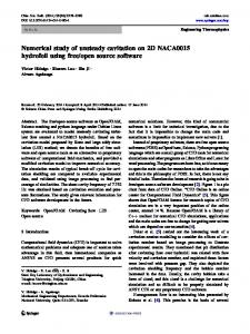
are given in Table 1. The quantity csinus is set to 3.15 m/s following equation (21). The quantity dPvap /dT is determined using the NIST thermodynamic table (Linstrom and Mallard, 2001). Figure 3 presents the linear approximation of the vapour pressure on the temperature interval [19, 24] K. The value of dPvap /dT is set to 38,980 Pa/K. For all simulations, the mesh contains 5,000 cells and the time step is set to 10−7 s. Computations are performed using the first-order Rusanov scheme. Figure 3 Variation of the vapour pressure with the temperature on the interval [19,24] K y = 0,38982x - 6,85898

3 2,5 2 Pvap (bar)

The double rarefaction tube

Figure 1

45

1,5 1

Wave propagation diagram of the expansion tube

Figure 2

0,5 0 19

20

21

22

23

24

Temperature (K)

A simple heat balance between the two phases can estimate the scale of temperature difference ∆T ∗ caused by thermal effects. ∆T ∗ =

ρv Lvap , ρl Cpl

(33)

where Lvap is the latent heat. The B-factor is estimated as the ratio between the actual temperature drop and ∆T ∗ . By assuming that the whole liquid contributes to the heat necessary for the vapour, we obtain (Franc and Michel, 2004): B =

∆T α ≃ . ∗ ∆T 1−α

(34)

However, the hypothesis that the whole liquid is contributing to the vapourisation process is a very strong one.

4.1 Initial velocity u0 =10 m/s A double rarefaction case is proposed for which the running fluid is liquid hydrogen in cryogenic conditions. Liquid hydrogen is initially at the pressure two bar and at the reference temperature Tref = 22.1 K. A weak volume fraction of vapour α = 0.01 is initially added to the liquid. The initial discontinuity velocity is u0 = 10 m/s. The vapour pressure at the reference temperature is Pvap (Tref ) = 1.63 bar. Parameters of the stiffened gas

The pressure, the void fraction, the temperature and the velocity are plotted in Figure 4, at time t = 0.8 ms, for both 4-equation models. The four expansion waves are clearly illustrated (two fast expansion waves and two slow evaporation fronts). The pressure drop under the initial value of the vapour pressure is around 0.2 bar. It is more pronounced using the 4-equation SG model and due to a larger cooling effect. The creation of void ratio is weak (around 20%) and a little more void ratio is produced by the 4-equation sinus model. For the velocity profile, results obtained with both models are similar. The vapour density ρv , the mass fraction of vapour Y , the B-factor and the speed of sound are plotted in Figure 5, at time t = 0.8 ms, for both 4-equation models. The mixture speed of sound of the sinus EOS is largely smaller than the SG relation, that can explain the greater quantity of vapour created by the sinus model, as observed for the mass fraction profile. Indeed, the mass transfer is linked to the quantity 1 − c2 /c2wallis following equation (10). The B-factor is computed as the ratio between the actual temperature drop and the characteristic temperature drop ∆T ∗ , following equation (34). Saturation values at the reference temperature Tref are used. For the 4-equation sinus, the maximal value is 0.375 to be compared with the ideal value given by the ratio α/(1 − α) = 0.31 evaluated with the maximal value of the void ratio (21% of error). For the 4-equation SG model, the maximal value is 0.49 to be compared with 0.22 (120% of error). Comparatively, the 4-equation sinus solution is in better agreement with the ideal value. The vapour density evolution is linked to the pressure and temperature profiles (it follows the stiffened gas EOS). As observed for T and P , the 4-equation SG model provides a lower value in comparison with the 4-equation sinus model.

E. Goncalvès and D. Zeidan

46

Finally, the effect of the numerical scheme is shown in Figure 6 where are plotted the pressure, the void ratio, the temperature and the velocity at time t = 0.8 ms. For all variables, numerical solutions obtained with both schemes are similar. A small difference can be observed on the expansion fronts, which are stiffer using the 2nd-order Jameson scheme. In the following, only simulations performed with the Rusanov scheme will be presented.

4.2 Initial velocity u0 =100 m/s The same conditions are used except regarding the discontinuity velocity which is set to u0 =100 m/s. Such high velocities are representative of flows occurring in turbopumps of rocket propulsion systems (see for example, Goncalves et al., 2010). In this case, evaporation is much more intense resulting in a large cavitation pocket.

Double rarefaction with cavitation in LH2 , u0 =10 m/s, t = 0.8 ms

Figure 4

10

2

0

4-eqt SG 4-eqt sinus

alpha

P (bar)

1.8

1.6

10

-1

1.4

1.2

0

0.2

0.4

x (m)

0.6

0.8

10-2

1

22.2

0.4

x (m)

0.6

0.8

1

5

21.8

u (m/s)

T (K)

0.2

10

22

21.6

0

-5

21.4 21.2

0

0

0.2

0.4

x (m)

0.6

0.8

-10

1

0

0.2

0.4

x (m)

0.6

0.8

1

Notes: Models comparison. Pressure, void ratio, temperature and velocity. Double rarefaction with cavitation in LH2 , u0 =10 m/s, t = 0.8 ms

Figure 5

0.01 4-eqt SG 4-eqt sinus

0.008

2.2

0.006 Y

3

rhov (kg/m )

2.4

2

0.004

1.8

0.002

1.6

0

0.2

0.4

x (m)

0.6

0.5

0.8

0

1

0.2

0.4

x (m)

0.6

0.8

1

4-eqt SG 4-eqt sinus

0.4

400

0.3

c (m/s)

B-factor

0

0.2

200

0.1 0

0

0.2

0.4

x (m)

0.6

0.8

1

0

0

0.2

Notes: Models comparison. Vapor density, mass fraction of vapour, B-factor and speed of sound.

0.4

x (m)

0.6

0.8

1

Numerical simulation of unsteady cavitation in liquid hydrogen flows

47

Double rarefaction with cavitation in LH2 , u0 =10 m/s, t = 0.8 ms

Figure 6

10

2

0

Jameson Rusanov

alpha

P (bar)

1.8 10

-1

1.6

1.4

0

0.2

0.4

0.6

x (m)

0.8

10-2

1

22.2

0.4

x (m)

0.6

0.8

1

5

21.8

u (m/s)

T (K)

0.2

10

22

21.6

0

-5

21.4 21.2

0

0

0.2

0.4

x (m)

0.6

0.8

-10

1

0

0.2

0.4

x (m)

0.6

0.8

1

Notes: Numerical schemes comparison. Pressure, void ratio, temperature and velocity. Figure 7

Variation of the vapour pressure with the temperature on the interval [14, 22] K y = 0,24540x - 3,73423

2

Pvap (bar)

1,5

1

0,5

0 14

15

16

17

18

19

20

21

22

Temperature (K)

The estimation of the slope dPvap /dT leads to difficulties due to the large temperature drop. A linear approximation on the temperature interval [14, 22] K is presented in Figure 7. The value of dPvap /dT is around 24,500 Pa/K. A parabolic approximation will be clearly better, but the model properties, especially the mixture speed of sound formulation, are more difficult to study. Secondly, using the linear approximation, we observe than the vapour pressure becomes negative if the temperature is smaller than 15 K. This situation occurs with the initial discontinuity velocity u0 =100 m/s. The pressure and the temperature are plotted in Figure 8, at time t = 0.8 ms, using the 4-equation sinus model with dPvap /dT = 24,500 Pa/K. The cooling effect is important and the mixture temperature decreases to 14.9 K. Negative

values of the pressure appear in the middle of the tube. A similar result is obtained using the 4-equation SG model. As a remedy, a smaller value is considered: Pvap /dT = 20,000 Pa/K. The pressure, the void fraction, the temperature and the vapour density are plotted in Figure 9, at time t = 0.8 ms, for both 4-equation models. Using the 4-equation SG model, negative values for the pressure and the vapour density are obtained. The temperature decreases up to 13.5 K that is lower than the triple point (13.8 K). On the other hand, using the 4-equation sinus model, the pressure and the vapour density remain positive. The temperature decreases to 14.3 K. The pressure drop under the initial value of the vapour pressure is very strong, it reaches 1.5 bar. A large cavitation area is created for which the maximal value of the void ratio is 84%.

48

E. Goncalvès and D. Zeidan

Figure 8

Double rarefaction with cavitation in LH2 , u0 =100 m/s, t = 0.8 ms 2

22

dP/dT=24500 Pa/K

20 T (K)

P (bar)

1.5

1

18

0.5

0

16

0

0.2

0.4

x (m)

0.6

0.8

14

1

0

0.2

0.4

0

0.2

0.4

0

0.2

0.4

x (m)

0.6

0.8

1

0.6

0.8

1

0.6

0.8

1

Notes: 4-equation sinus model, dPvap /dT = 24, 500 Pa/K. Pressure and temperature. Double rarefaction with cavitation in LH2 , u0 =100 m/s, t = 0.8 ms

Figure 9 2

10

4-eqt SG 4-eqt sinus

0

alpha

P (bar)

1.5 1

10

-1

0.5 0 0

0.2

0.4

x (m)

0.6

0.8

10-2

1

2.5

20

2

T (K)

3

rhov (kg/m )

22

18 16

x (m)

1.5 1

0.5

14 0 12

0

0.2

0.4

x (m)

0.6

0.8

1

x (m)

Notes: Models comparison, dPvap /dT = 20,000 Pa/K. Pressure, void ratio, temperature and vapour density. Figure 10 Double rarefaction with cavitation in LH2 , u0 =100 m/s, t = 0.8 ms 6

dP/dT=20000 Pa/K

dP/dT=20000 Pa/K 400

4 c (m/s)

B-factor

5

3

200

2 1 0

0.2

0.4

x (m)

0.6

0.8

1

0

0.2

0.4

x (m)

0.6

0.8

1

Note: 4-equation sinus model. B-factor and speed of sound

Figure 12 presents the B-factor and the mixture speed of sound evolutions in the tube, at time t = 0.8 ms, computed with the 4-equation sinus model and with dPvap /dT = 20,000 Pa/K. The maximal value of the B-factor is 5.5 to be compared with the ideal value estimated with the maximal void ratio (84%) that is 5.25 (5% of error). The numerical simulation is in close

agreement with the theoretical value. The large variations of the speed of sound are well illustrated: around 460 m/s in the initial condition, 12 m/s behind the expansion waves and 146 m/s in the cavitation area. This non-monotonous behaviour makes the numerical integration stiff.

Numerical simulation of unsteady cavitation in liquid hydrogen flows

49

Figure 11 Double linear approximations of Pvap (T ) on the interval [14, 22] K 2 y = 0,27263x - 4,48093

Pvap (bar)

1,5

1 y = 0,09727x - 1,31635

0,5

0 14

15

16

17

18

19

20

21

22

0

0.2

0.4

0

0.2

0.4

Temperature (K)

Double rarefaction with cavitation in LH2 , u0 =100 m/s, t = 0.8 ms

Figure 12 2

10

4-eqt SG 4-eqt sinus

0

alpha

P (bar)

1.5 1

10

-1

0.5 0 0

0.2

0.4

x (m)

0.6

0.8

10-2

1

2.5

20

2

T (K)

3

rhov (kg/m )

22

18 16

x (m)

0.6

0.8

1

0.6

0.8

1

1.5 1

0.5

14 0 12

0

0.2

0.4

x (m)

0.6

0.8

1

x (m)

Notes: Models comparison, splitting of linear approximation of dPvap /dT . Pressure, void ratio, temperature and vapour density.

Another strategy for the estimation of dPvap /dT consists in splitting the linear approximation on two intervals, as plotted in Figure 10. The temperature at the intersection between the two lines is 18.15 K. Values of dPvap /dT are 9,930 Pa/K and 27,260 Pa/K, respectively. The pressure, the void fraction, the temperature and the vapour density are plotted in Figure 11, at time t = 0.8 ms, for both 4-equation models. Using the 4-equation SG model, as previously negative values are obtained for the pressure and vapour density. For both models, an irregularity is observed on profiles due to the change of slope dPvap /dT around 18 K. For the 4-equation sinus model, the temperature drop reaches 13.7 K, which is under the triple point value.

4.3 Shock-cavitation interaction, u0 =100 m/s This case is similar to the previous one, except that the two ends of the tube are simultaneously closed once the flow starts. Therefore, a shock created at each end moves towards the centre, resulting in shock-cavitation interaction and cavitation collapse. A uniform mesh of 5,000 cells is used and the time step is set to 10−8 s. Simulations are performed using the 4-equation sinus model with dPvap /dT = 20, 000 Pa/K.

E. Goncalvès and D. Zeidan

50

Figure 13 Shock-cavitation interaction, u0 =100 m/s, t = 1.2 ms 1 1

0.8

100

10

t=0.5ms t=0.6ms t=0.8ms t=1.0ms t=1.1ms t=1.2ms

-1

10-2 0.2

0.4

x (m)

0.6

0.6

alpha

P (bar)

10

0.4 0.2

0.8

0.4

0.45

0.5 x (m)

0.55

0.6

35 10 rhov (kg/m3)

T (K)

30 25 20 15 0.2

100

10

0.4

x (m)

0.6

1

-1

10-2 0.2

0.8

0.4

x (m)

0.6

0.8

Notes: 4-equation sinus model, dPvap /dT = 20,000 Pa/K. Pressure, void ratio, temperature and vapour density.

The pressure, the void ratio, the temperature and the vapour density are plotted at different times in Figure 13 (with a logarithmic scale for the pressure and the vapour density). The cavitation pocket grows up to time t = 0.6 ms. After this time, the shocks created at the ends meet the rarefaction waves generated at the centre, and then interacts with the expanding cavitation interface. The cavitation collapse begins. The reduction of the cavitation area is clearly observed on the void ratio profile after time t = 0.6 ms. From time 0.6 ms to 1.1 ms, the cavitation pocket narrows but the maximal void ratio remains around 80%. At time t = 1.2 ms, the decrease of the void ratio is abrupt and the value in the middle of the tube is around 5%. The shock propagation through the rarefaction region is well illustrated on the pressure, the temperature and the vapour density profiles, up to time t = 0.6 ms. Then shocks interacts with the expanding cavitation interface, resulting in a discontinuity forms at the interface. The cavitation collapse generates two shocks which propagate outwards. For the initial shocks, the maximum pressure is around 54 bar, whereas the maximal pressure for the two shocks created during the cavitation collapse is around 28 bar. At time t = 1.2 ms when the void ratio decreases abruptly, we observe a large increase of the vapour density up to 28 kg/m3 and a warming effect about 6 K in comparison with the reference temperature. At time t = 1.3 ms (not presented), the temperature reaches 30 K. The magnitude of both phenomena, the cooling effect due to the evaporation and the warming effect due to the collapse, is quite similar.

5 Conclusions The thermal effects in 1D cryogenic cavitating flows were studied. Two EOS were tested associated with a mass transfer closure based on the ratio between the mixture speed of sound and the Wallis speed of sound. Simulations were performed on inviscid rarefaction problems leading to a phase transition, for which the working fluid is liquid hydrogen at the temperature 22.1 K. Different initial velocities were considered and especially a high-speed case was investigated, corresponding to a realistic velocity in turbopump applications. Moreover, a shock-cavitation case was simulated leading to the collapse of the cavitation area. These cases lead to different concluding remark: •

As regard to the EOS comparison, the sinus model generated more vapour and a lower temperature depression than the SG model. For the high-speed case, the pressure and vapour density obtained with the SG model were negative, that constitutes a clear drawback.

•

Problems appeared with the calibration of the parameter dPvap /dT for the high-speed case because of the prediction of negative pressure. A piecewise approximation was tested and led to a temperature decrease lower than the triple point value. For this situation, a specific thermodynamic model have to be developped. Using a constant value dPvap /dT = 20, 000 Pa/K, the simulated temperature drop was around 8K and the result was in good agreement with the B-factor theory.

Numerical simulation of unsteady cavitation in liquid hydrogen flows •

For the shock-cavitation case, a warming effect was highlighted during the collapse for which the magnitude was quite similar to the cooling effect during the evaporation process.

Ongoing works are to pursue comparative analysis and to develop two-temperature models. A detailed thermal analysis under a range of physical conditions is planned in later phases of work to be reported in future publications.

Acknowledgements The authors gratefully acknowledge support from the German Jordanian University and ENSMA – Pprime.

References Allaire, G., Clerc, S. and Kokh, S. (2002) ‘A five-equation model for the simulation of interfaces between compressible fluids’, Journal of Computational Physics, Vol. 181, No. 2, pp.577–616. Ambroso, A., Chalons, C. and Raviart, P-A. (2012) ‘A Godunov-type method for the seven-equation model of compressible two-phase flow’, Computers and Fluids, Vol. 54, pp.67–91. Baer, M. and Nunziato, J. (1986) ‘A two-phase mixture theory for the deflagration-to-detonation transition (DDT) in reactive granular materials’, Int. Journal of Multiphase Flow, Vol. 12, No. 6, pp.861–889. Barberon, T. and Helluy, P. (2005) ‘Finite volume simulation of cavitating flows’, Computers & Fluids, Vol. 34, No. 7, pp.832–858. Causon, D. and Mingham, C. (2013) ‘Finite volume simulation of unsteady shock-cavitation in compressible water’, Int. Journal of Numerical Methods in Fluids, Vol. 72, No. 6, pp.632–649. Chalons, C., Coquel, F., Kokh, S. and Spillane, N. (2011), Large time-step numerical scheme for the seven-equation model of compressible two-phase flows’, in Finite Volumes for Complex Applications VI Problems and Perspectives Springer Proceedings in Mathematics Volume’, Vol. 4, pp.225–233. Charriere, B., Decaix, J. and Goncalves, E. (2015) ‘A comparative study of cavitation models in a venturi flow’, European Journal of Mechanics – B/Fluids, Vol. 49, Part A, pp.287–297. Downar-Zapolski, P., Bilicki, Z., Bolle, L. and Franco, J. (1996) ‘The non-equilibrium relaxation model for one-dimensional flashing liquid flow’, Int. Journal of Multiphase Flow, Vol. 22, No. 3, pp.473–483. Florschuetz, L. and Chao, B. (1965) ‘On the mechanics of vapor bubble collapse’, Journal of Heat Transfer, Vol. 87, No. 2, pp.209–220. Franc, J-P. and Michel, J-M. (2004) Fundamentals of Cavitation, Springer, Netherlands. Fujikawa, S., Okuda, M. and Akamatsu, T. (1980) ‘Non-equilibrium vapour condensation on a shock-tube endwall behind a reflected shock wave’, Journal of Fluid Mechanics, Vol. 183, pp.pp.293–324.

51

Goncalves, E. and Charriere, B. (2014) ‘Modelling for isothermal cavitation with a four-equation model’, International Journal of Multiphase Flow, Vol. 59, pp.54–72. Goncalves, E. and Patella, R.F. (2009) ‘Numerical simulation of cavitating flows with homogeneous models’, Computers & Fluids, Vol. 38, No. 9, pp.1682–1696. Goncalves, E. and Patella, R.F. (2010) ‘Numerical study of cavitating flows with thermodynamic effect’, Computers & Fluids, Vol. 39, No. 1, pp.99–113. Goncalves, E. and Zeidan, D. (2015) ‘Numerical study of cavitation in liquid hydrogen flow’, in Proceedings of the 8th International Conference on Thermal Engineering Theory and Applications, Amman-Jordan, May 18–21, pp.13. Goncalves, E., Patella, R.F., Rolland, J., Pouffary, B. and Challier, G. (2010) ‘Thermodynamic effect on a cavitating inducer in liquid hydrogen’, Journal of Fluids Engineering, Vol. 132, No. 11, pp.111305. Goncalves, E. and Patella, R.F. (2011) ‘Constraints on equation of state for cavitating flows with thermodynamic effects’, Applied Math. and Computation, Vol. 217, No. 11, pp.5095–5102. Goncalves, E. (2013) ‘Numerical study of expansion tube problems: toward the simulation of cavitation’, Computers & Fluids, Vol. 72, pp.1–19. Goncalves, E. (2014) ‘Modeling for non isothermal cavitation using 4-equation model’, International Journal of Heat and Mass Transfer, Vol. 76, pp.247–262. Hsiao, C. and Chahine, G. (2002) ‘Prediction of vortex cavitation inception using coupled spherical and non-spherical models and unrans computations’, in Proceedings of the 24th Symposium on Naval Hydrodynamics. Hsiao, C., Jain, A. and Chahine, G. (2006) ‘Effect of gas diffusion on bubble entrainment and dynamics around a propeller’, in Proceedings of the 26th Symposium on Naval Hydrodynamics, Rome, Italy. Huang, B., Wu, Q. and Wang, G. (2014) ‘Numerical investigation of cavitating flow in liquid hydrogen’, Int. Journal of Hydrogen Energy, Vol. 39, No. 4, pp.1698–1709. Ishimoto, J. and Kamijo, K. (2004) ‘Numerical study of cavitating flow characteristics of liquid helium in a pipe’, Int. Journal of Heat and Mass Transfer, Vol. 47, pp.pp.149–163. Jameson, A., Schmidt, W. and Turkel, E. (1981) Numerical Solution of the Euler Equations by Finite Volume Methods using Runge-Kutta Time Stepping Schemes, AIAA Paper 81–1259. Kapila, A., Menikoff, R., Bdzil, J., Son, S. and Stewart, D. (2001) ‘Two-phase modeling of deflagration-to-detonation transition in granular materials: reduced equations’, Physics of fluids, Vol. 13, No. 10, pp.3002–3024. Kreeft, J. and Koren, B. (2010) ‘A new formulation of Kapila’s five-equation model for compressible two-fluid flow, and its numerical treatment’, Journal of Computational Physics, Vol. 229, No. 18, pp.6220–6242. Linstrom, P.J. and Mallard, W.G. (2001) ‘The NIST Chemistry WebBook: a chemical data resource on the internet’, J. Chem. Eng. Data, Vol. 46, No. 5, pp.1059–1063, DOI: 10.1021/je000236i. Metayer, O.L., Massoni, J. and Saurel, R. (2004) ‘Elaborating equations of state of a liquid and its vapor for two-phase flow models’, Int. Journal of Thermal Sciences, Vol. 43, No. 3, pp.265–276.

52

E. Goncalvès and D. Zeidan

Moore, R. and Ruggeri, R. (1968) Prediction of Thermodynamic Effects on Developed Cavitation based on Liquid Hydrogen and Freon 114 Data in Scaled Venturis, Technical report, NASA, TM D-4899. Pelanti, M. and Shyue, K. (2014) ‘A mixture-energy-consistent six-equation two-phase numerical model for fluids with interfaces, cavitation and evaporation waves’, Journal of Computational Physics, Vol. 259, pp.331–357. Prosperetti, A. and Plesset, M. (1978) ‘Vapour-bubble growth in a superheated liquid’, Journal of Fluid Mechanics, Vol. 85, No. 2, pp.349–368. Rodio, M., Giorgi, M.D. and Ficarella, A. (2012) ‘Influence of convective heat transfer modeling on the estimation of thermal effects in cryogenic cavitating flows’, Int. Journal of Heat and Mass Transfer, Vol. 55, Nos. 23–24, pp.6538–6554. Rusanov, V. (1961) ‘Calculation of interaction of non-steady shock waves with obstacles’, Journal of Computational Mathematics and Physics, Vol. 1, pp.267–279. Saurel, R. and Metayer, O.L. (2001) ‘A multiphase model for compressible flows with interfaces, shocks, detonation waves and cavitation’, Journal of Fluid Mechanics, Vol. 431, pp.239–271. Saurel, R., Petitpas, F. and Abgrall, R. (2008) ‘Modelling phase transition in metastable liquids: application to cavitating and flashing flows’, Journal of Fluid Mechanics, Vol. 607, pp.313–350. Schmidt, D., Gopalakrishnan, S. and Jasak, H. (2010) ‘Multi-dimensional simulation of thermal non-equilibrium channel flow’, International Journal of Multiphase Flow, Vol. 36, No. 4, pp.284–292.

Spina, G.L., de Mihieli Vitturi, M. and Romenski, E. (2014) ‘A compressible single-temperature conservative two-phase model with phase transitions’, Int. Journal of Numerical Methods in Fluids, Vol. 76, No. 5, pp.282–311. Stahl, H., Stepanoff, A. and Phillipsburg, N. (1956) ‘Thermodynamic aspects of cavitation in centrifugal pumps’, Journal of Fluids Engineering, Vol. 78, pp.1691–1693. Tseng, C. and Shyy, W. (2010) ‘Modeling for isothermal and cryogenic cavitation’, Int. Journal of Heat and Mass Transfer, Vol. 53, Nos. 1–3, pp.513–525. Utturkar, Y., Wu, J., Wang, G. and Shyy, W. (2005) ‘Recent progress in modelling of cryogenic cavitation for liquid rocket propulsion’, Progress in Aerospace Sciences, Vol. 41, No. 7, pp.558–608. Wallis, G. (1967) One-dimensional Two-phase Flow, McGraw-Hill, New York. Zeidan, D., Romenski, E., Slaouti, A. and Toro, E. (2007) ‘Numerical study of wave propagation in compressible two-phase flow’, International Journal for Numerical Methods in Fluids, Vol. 54, No. 4, pp.393–417. Zein, A., Hantke, M. and Warnecke, G. (2010) ‘Modeling phase transition for compressible two-phase flows applied to metastable liquids’, Journal of Computational Physics, Vol. 229, No. 8, pp.2964–2998.