Numerical simulation scheme of one-and two-dimensional ... - HAL-Inria

Numerical simulation scheme of one-and two-dimensional neural fields involving space-dependent delays Axel Hutt, Nicolas P. Rougier

To cite this version: Axel Hutt, Nicolas P. Rougier. Numerical simulation scheme of one-and two-dimensional neural fields involving space-dependent delays. P. Beim Graben and S. Coombes and R. Potthast and J.J. Wright. Neural Field Theory, Springer, 2014.

HAL Id: hal-00872132 https://hal.inria.fr/hal-00872132 Submitted on 7 Jan 2014

HAL is a multi-disciplinary open access archive for the deposit and dissemination of scientific research documents, whether they are published or not. The documents may come from teaching and research institutions in France or abroad, or from public or private research centers.

L’archive ouverte pluridisciplinaire HAL, est destin´ee au d´epˆot et `a la diffusion de documents scientifiques de niveau recherche, publi´es ou non, ´emanant des ´etablissements d’enseignement et de recherche fran¸cais ou ´etrangers, des laboratoires publics ou priv´es.

Numerical simulation scheme of one- and two dimensional neural fields involving space-dependent delays Axel Hutt Inria CR Grand Est - Nancy, Villers-les-Nancy, France Nicolas Rougier Inria, Bordeaux Sud-Ouest, France LaBRI, UMR 5800 CNRS, Bordeaux University Institute of Neurodegenerative Diseases, UMR 5293 September 5, 2013

1 Introduction Finite transmission speed in physical systems has attracted research for decades. Previous work on heat diffusion has shown experimentally that the transmission speed (also called propagation speed in the literature) is finite in certain media [16, 14]. These results do not show accordance to classical diffusion theory implying infinite transmission speed. To cope with this problem theoretically, Cattaneo was one of the first to insert delay terms into the diffusion equation to achieve a finite transmission speed [5]. Recently, an integral model has been proposed which takes into account a finite transmission speed as a space-dependent retardation [10]. It was shown that the Cattaneo-equation can be derived from this model. This model is well-established in computational neuroscience and known as the neural field model. It describes the activity evolution in a neural population involving finite transmission speed along axonal fibres. The neural field model has been shown to model successfully neural activity known from experiments [9, 3]. In the recent decades, neural 1

fields have been studied analytically and numerically in one and two spatial dimensions [19, 15], while previous studies considered finite axonal transmission speeds in one-dimensional models only [6, 11, 1, 2]. To our best knowledge, only few previous studies considered analytically and numerically finite transmission speeds in two-dimensional neural fields. The current work presents a recently developed method [13] to reveal finite transmission speed effects in two-dimensional systems. The subsequent paragraphs derive a novel fast numerical scheme to simulate the corresponding evolution equations in one and then in some detail in two spatial dimensions. Stimulus-induced activity propagation in two spatial dimensions is studied numerically to illustrate the delayed activity spread. We find numerically transmission delay-induced breathers. The underlying model considers a one-dimensional line Ω with length l or a two-dimensional rectangle spatial domain Ω with side length l, in both cases assuming periodic boundary conditions. In addition, the center of the coordinate system is chosen to be the center of the domain in the following. Then the neural population activity V (x,t), i.e. the mean membrane potential, at spatial location x 2 Ω and time t obeys the evolution equation ◆%  ✓ Z |x − y| ∂ n (1) τ V (x,t) = I(x,t) −V (x,t) + d y K(|x − y|)S V y,t − ∂t c Ω with n = 1 or n = 2, the synaptic time constant τ, the external stimulus I(x,t), the finite axonal transmission speed c and the nonlinear transfer function S. Moreover, the spatial interaction is non-local and is given by the spatial synaptic connectivity kernel K(|x−y|), that depends on the distance between two spatial locations x and y only.

2

2 The novel principle For notational simplicity, let us consider a one-dimensional spatial domain. Then the integral on the right hand side of Eq. (1) can be re-written as  ✓ ◆% Z |x − z| dz K(|x − z|)S V z,t − c Ω ◆ ✓ Z ∞ Z |x − z| 0 0 = dz − (t − t ) K(|x − z|)S[V (z,t 0 )] dt δ c Ω −∞ = =

Z

dz

Ω

Z

Ω

Z ∞

−∞

dz

dt 0 L(x − z,t − t 0 )S[V (z,t 0 )]

Z τmax 0

dτL(x − z, τ)S[V (z,t − τ)],

with τmax = l/c. This shows that the introduction of the space-time kernel L(x,t) = K(x)δ (|x|/c − t) allows us to write the single space integral as two integrals: one spatial convolution and one integral over delays. To understand the logic of the computation, let us discretize the time and space by t ! tn = n∆t, x ! xm = m∆x with n 2 N0 , m 2 Z0 , |m| < M/2 and l = M∆x. This implies that the speed c also takes discrete values. We obtain L(x,t) ! L(xm ,tn ) ⇠ K(m∆x)δ ((∆x/c)|m| − n∆t) ◆◆ ✓ ✓ ∆x |m| − n = Km δ ∆t c∆t = Km δ (∆t (r|m| − n)) = Km δ (|m|∆t (r − n/|m|)) ⇠ Km δ|m|,n/r with Km = K(m∆x), r = ∆x/(c∆t). The last equation shows that L(xm ,tn ) ⇠ K±n/r 6= 0 only if r is rational number with r = n/m and thus c =

∆x 1 ∆x m = ∆t r ∆t n

is discrete.

3

3 The numerical implementation in two spatial dimensions To investigate the activity propagation in detail, we derive a novel iteration scheme for the numerical integration of (1) for n = 2. Since the integral over space in (1) is not a convolution in the presence of a finite transmission speed c, one can not apply directly fast numerical algorithms such as the Discrete Fast Fourier Transform (DFT) to calculate the integral. Hence the numerical integration of (1) is very time consuming with standard quadrature techniques. For instance, with a discretization of the spatial domain by N 2 grid intervals and applying the Gaussian quadrature rule for the spatial integral, it would be necessary to compute N 4 elements in each time step which is very time-consuming in the case of a good spatial resolution. The work [13] proposes a fast numerical method that is based on the DFT and resembles the Ritz-Galerkin method well-established to solve partial differential equations. As in the previous section, the integral in (1) reads  ✓ ◆% Z |x − y| 2 A(x,t) = d y K(|x − y|)S V y,t − c Ω ◆ ✓ Z Z ∞ |x − y| − (t − t 0 ) K(|x − y|)S[V (y,t 0 )] dt 0 δ = d2y c −∞ Ω = =

Z

2

d y

Ω

Z

Ω

Z ∞

−∞

d2y

dt 0 L(x − y,t − t 0 )S[V (y,t 0 )]

Z τmax 0

dτL(x − y, τ)S[V (y,t − τ)],

(2) (3)

p with τmax = l/ 2c, the novel spatial delay kernel L(x, τ) = K(x)δ (|x|/c − τ) and the delta-distribution δ (·). These simple calculations show that A may be written as a two-dimensional spatial convolution, but with a new delayed spatio-temporal kernel L that now considers the past activity. The form (2) has been used previously to study spatio-temporal instabilities in one- and two-dimensional neural fields [19]. The new delay kernel L is independent of time t and is computed on the delay interval only. Hence it represents the contribution of the current and past activity to the current activity at time t. In addition A implies multiple delays and the corresponding delay distribution function depends strongly on the spatial kernel K. In other words, axonal transmission speeds represent a delay distribution as found before in other contexts [12, 7]. 4

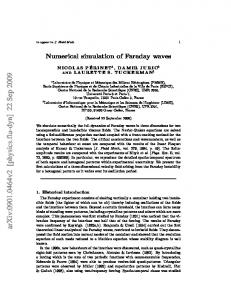
L4 L3

K

L2 L1 L0 t v∆

v∆

t

ti m

e

Figure 1: The construction of the delay-kernel L(x, τ). Assuming a spatial kernel (left image), L exhibits rings with radius cτ (images on the right for different delay times) which is the interaction distance of the system at the delay time τ. Figure 1 illustrates the construction of the kernel: given the kernel function K in space (Fig. 1, left), L(x, τ) is generated by cutting out a ring of radius cτ (Fig. 1, right hand side). In a continuous spatial domain these rings are infinitely thin, whereas a spatially discretized domain yields finite ring widths, see the paragraphs below for more details. Now let us derive the rules to compute A numerically. The periodic boundary conditions implied lead to discrete wave vectors kmn = (km , kn ) with k p = 2π p/l, p 2 Z0 . The Fourier series of V (x,t) reads V (x, y,t) =

1 ∞ ˜ ∑ Vmn(t)ei(kmx+kny) l m,n=−∞

(4)

with the Fourier vector component V˜mn (t) = V˜ (km , kn ,t) and the spatial Fourier transform 1 V˜mn (t) = l

Z l/2

−l/2

dx

Z l/2

−l/2

5

dyV (x, y,t)e−i(km x+kn y) .

(5)

Inserting (4) into (3) and applying (5) leads to ∞

∑

A(x, y,t) =

i(km x+kn y)

e

Z τmax 0

m,n=−∞

dT L˜ mn (T )S˜mn (t − T ),

(6)

with the spatial Fourier transforms of L(x,t) L˜ mn (t), S˜mn (t) and the nonlinear functional S[V (x,t)]. Moreover c2 L˜ mn (T ) = l

Z l/2c Z l/2c

−l/2c −l/2c

δ (|τ| − T )K(|cτ|)e−ickmn τ d 2 τ .

(7)

After obtaining A(x, y,t) in the Fourier space for a continuous spatial domain, now we discretize the spatial domain to gain the final numerical scheme. To this end, Ω is discretized in a regular spatial grid of N ⇥ N elements with grid interval ∆x = l/N. Hence x ! xn = n∆x, n = −N/2, . . . , N/2 − 1. By virtue of this discretization, we can approximate (6) and (7) by applying the rectangular rule Rb N/2−1 2 00 a f (x)dx ⇡ ∆x ∑n=−N/2 f (xn ). The error is E < (b − a)∆x f (ξ )/24, a < ξ < b for twice-differentiable functions f , i.e. the rectangular rule is a good approximation for smooth functions and large enough N. The same holds true for the discretization of the time integral and Eq. (7) reads L˜ mn (Tu ) =

N/2 l Lkp (Tu ) e−i2π(km+np)/N ∑ 2 N ∆t k,p=−N/2

(8)

with the discrete version of the delay kernel L p Lkp (Tu ) = δ (∆τ k2 + p2 , Tu )K(|xkp |).

The symbol δ (·, ·) is identical to the Kronecker symbol and is introduced for notational convenience. By virtue of the isotropy of the spatial interactions, in addition we find the simple relation Lkp (Tu ) = K(uc∆t). In other words the width of the rings in Fig. 1 is c∆t. In these latter calculations, we introduced the time discretization τ kp = (k, p)∆τ, ∆τ = ∆x/c, T ! Tu = u∆t and δ (τ − T ) ! δnu /∆t for τ ! τn . Although the relation Lkp (Tu ) = K(uc∆t) seems to be quite intuitive and elucidates the discrete ring structure of L, it does not give directly the condition which 6

grid point (k, p) belongs to which delay ring. This conditionpmay be read off the Kronecker symbol: u is an integer number and hence δ (∆τ k2 + p2 , Tu ) = 1 p if [∆τ k2 + p2 /∆t] = u with the integer operation [a] that cuts off the decimal numbers. Consequently the grid points (k, p) that contribute to the delay time Tu obey u

∆x p 2 k + p2 < u + 1, u = 0, 1, 2, . . . , umax c∆t

with umax = [τmax /∆t], i.e. they lie in a ring with inner and outer radius (c∆t/∆x)u and (c∆t/∆x)(u + 1), respectively. Moreover, the definition of Lkp (Tu ) allows us to derive some conditions on the numerical parameters. The ring width in Fig.1 is ∆r = c∆t/∆x which p is the number of spatial grid intervals. Hence the maximum radius of a ring is l/ 2∆x andp hence the maximum transmission speed that can be implemented is cmax = l/ 2∆t. Since cmax ! ∞ for ∆t ! 0, the transmission speed c > cmax in the discrete scheme is equivalent to an infinite transmission speed in the analytical original model and the finiteness of cmax results from the time discretization. Moreover, c ! cmax yields τmax ! 0, i.e. the transmission delay vanishes. We add that the maximum wave number is kmax = 2π/∆x and, by the definition of ∆x, the number of Fourier modes is limited to N. Combining the latter results now Eq. (6) reads N/2−1

∑

A(xr , ys ,tv ) =

i2π(mr+ns)/N

e

m,n=−N/2

⇥

umax −1

∑

u=0

L˜ mn (Tu )S˜mn (tv − Tu ) .

(9)

With the standard definition of the two-dimensional Discrete Fourier Transform DFT [A]kp = ∑ Anm e−i2π(nk+mp)/N , n, m 2 [−N/2; N/2 − 1] n,m

and its inverse (IDFT) correspondingly, we find finally " # umax −1 l2 IDFT ∑ DFT [L(Tu )] ⇥ DFT [S(tv − Tu )] . A(x,tv ) = N2 u=0

(10)

Some numerical implementations of the DFT assume that the index n runs in the interval [0; N − 1]. In this case, Eq. (10) is also valid but DFT [A]kp is modulated by a factor e−iπ(k+p) = (−1)k+p .

7

In practice, DFT [L(Tu )] is computed once for all Tu in the beginning of the simulation since it does not depend on the system activity. Moreover, for N = 2n , n 2 N , the discrete Fourier Transform may be implemented numerically by a Fast Fourier transform, that speeds up the numerical computation dramatically. This possible algorithm choice represents the major advantage of the proposed method compared to other non-convolution methods. The discrete version of A can be applied to any explicit or implicit numerical integration scheme. For instance, the numerical Euler scheme stipulates ∆t V˜mn (ti + ∆t) = V˜mn (ti ) + (Imn (ti ) − V˜mn (ti ) τ d 3 ∆t L + ∑ DFT [L(tu)]mn ⇥ DFT [S(tv − tu)]mn) τ N 4 u=0

(11)

where Imn (t) is the Fourier transform of the input I(x,t) and one obtains V (x,tv ) by applying Eq. (4). In the following, we study analytically and numerically the response to an external stimulus. At first, let us consider a small input. Then the response is linear about the systems’ stationary state. Since we are interested in responses that approach the stationary state after removal of the stimulus, it is necessary to ensure the linear stability of the stationary state. The stationary state of Eq. (1) constant in space and time implies V0 = κS[V0 ] + I0 R for a constant input I0 with the kernel norm κ = Ω K(x)d 2 x. Considering small ¯ additional external inputs I(x,t) = I(x,t) − I0 , small deviations u(x,t) = V (x,t) − V0 from this stationary state obey du(x,t) ¯ = −u(x,t) + I(x,t) + s0 dt

Z

Ω

K(x − y)u (y,t − |x − y|/c) dy2 . (12)

with s0 = δ S[V ]/δV,V = V0 . Now expanding u(x,t) into a spatial Fourier series according to Eq. (4) and applying a temporal Laplace transform to each Fourier mode amplitude, we find the characteristic equation λ +1 =

Z

Ω

K(x)eikx−λ |x|/c d 2 x

(13)

with the wave vector k = (km , kn )t and the Lyapunov exponent λ 2 C . The stationary state V0 is linearly stable if Re(λ ) < 0. 8

Now let us consider the spatio-temporal response of the system involving the spatially periodic interactions 2

K(x) = Ko ∑ cos(ki x) exp(−|x|/σ ) i=0

with ki = kc (cos(φi ), sin(φi ))t , φi = iπ/3 . This kernel reflects spatial hexagonal connections which have been found, e.g., in layer 2/3 of the visual cortex in monkeys [17]. Stimulating the stable system by a small external input in the presence of the finite transmission speed c elucidates the transmission delay effect on the linear response. This delay effect has attracted some attention in previous studies on the activity propagation in the visual cortex [18, 4]. For the given kernel, the characteristic equation (13) reads 2

λ + 1 = ∑ f+ (λ , φi ) + f− (λ , φi ) i=0

with q 3 f± (λ , φi ) = 1/ (1/σ + λ /c)2 + k2 + kc2 ± 2kkc cos(φi − θ )

and k = k(cos(θ ), sin(θ ))t . The numerical simulation applies parameters which guarantee the stability of the stationary state. Figure 2 shows snapshots of the simulated spatio-temporal response of the system about a stable stationary state applying the numerical scheme (11). We observe the lateral activity propagation starting from the stimulus location in the domain centre. The spreading activity reveals the maxima of axonal connections close to previous experimental findings [17]. To validate the numerical results, we take a closer look at two single spatial locations, denoted A and B in Fig. 2 at distance dA and dB from the stimulus location in the center. Before stimulus onset, they show the stationary activity constant in time. After stimulus onset, it takes the activity some time to propagate from the stimulus location to these distant points, e.g. the transmission delays dA /c = 3.3ms and dB /c = 6.2ms. Figure 2 shows that the activity reaches the locations A and B about these times for the first time as expected. This finding validates the numerical algorithm proposed above. 9

t=3.30ms

t=3.65ms

t=5.50ms

t=6.20ms

t=8.00ms

Figure 2: Spatio-temporal response activity to the external stimulus I(x,t) = 2 2 I0 + e−x /σI for the spatial connectivity function K(x) given by the numerical simulation of Eq. (1). Used (dimensionless) parameters are Ko = 0.1, c = 10, l = 10, kc = 10π/l, σ = 10, σI = 0.2, N = 512, τ = 1, ∆t = 0.005. Moreover, I0 = 2.0, S[V ] = 2/(1 + exp(−5.5(V − 3))) and V0 = 2.00083. The initial values are chop sen to V (x, θ ) = V0 for the delay interval −l/ 2c  θ  0. Introducing the temporal and spatial scale scale τ = 10ms and λ = 1.0mm, the results reflect the spatio-temporal activity with transmission speed c = 1.0m/s and the domain length l = 10mm, which are realistic values for layer 2/3 in visual cortex. Then the points A and B are located at a distance dA = 2.1mm and dB = 3.8mm from the stimulus onset location at the origin, respectively. The bar in the plots is 0.83mm long. We investigate whether the transmission delay induces oscillatory instabilities in the presence of external input. The following brief numerical study is motivated by previous theoretical studies on breathers [8]. In that study, the authors computed analytically conditions for Hopf-bifurcations from stimulus-induced stable standing bumps in a neural model involving spike rate adaption. The presence of the spike rate adaption permits the occurence of the Hopf-bifurcation. The corresponding control parameter of these instability studies is the magnitude of the applied external stimulus. In contrast, the present model does not consider spike rate adaption to gain a Hopf-bifurcation, but consider tranmsission delays. We decreases the axonal transmission speed from large speeds, i.e. increases the transmission delay, to evoke a delay-induced Hopf-bifurcation while keeping the other parameters constant. Let us assume an anisotropic Gaussian stimulus t −1 x/2

I(x,t) = I0 e−x Σ

2 with the 2 ⇥ 2 diagonal variance matrix Σ−1 with Σ−1 ii = 1/σi , i = 1, 2. Moreover the spatial kernel K(x) represents locally excitatory and laterally inhibitory connections and the transfer function is the Heaviside function S[V ] = H[V −Vthresh ]. The numerical computation of Eq. (1) applying the numerical scheme (11) yields

10

Figure 3: One cycle of a transmission delay-induced breathers evoked by an anisotropic external stimulus. The spatial connectivity function is chosen to K(r) = 10 exp(−r/3)/(18π) − 14 exp(−r/7)/(98π) and the input magnitude and −1 variances are I0 = 10 and Σ−1 11 = 3, Σ22 = 5, respectively. Other parameters are c = 100, l = 30, N = 512, τ = 1, ∆t = 0.05 and Vthresh p = 0.005. The initial values are chosen to V (x, θ ) = 0 for the delay interval −L/ 2c  θ  0. delay-induced breathers in two dimensions. Figure 3 shows the temporal sequence of a single oscillation cycle. To our best knowledge such delay-induced breathers in two dimensions have not been found before.

4 Conclusion We have motivated briefly a one-dimensional numerical method to integrate a spatial integral involving finite transmission speeds Moreover we have derived analytically and validated numerically in detail a novel numerical scheme for twodimensional neural fields involving transmission delay that includes a convolution structure and hence allows the implementation of fast numerical algorithms, such as Fast Fourier Transform. We have demonstrated numerically a transmission delay-induced breather [13]. To facilitate future applications of the algorithm, the implementation code for both numerical examples is made available for download1 . We point out that the method can be easily extended to higher dimensions. In future research, the transmission delay will play an important role in the understanding of fast activity propagations whose time scales are close to the transmission delay, e.g. in the presence of ultra-fast pulses and/or at spatial nanometer scales. An open source Graphical User Interface written in Python for a user1 http://www.loria.fr/

˜rougier/research/DNF.html

11

friendly application of the method proposed will be available soon2 .

References [1] F. M. Atay and A. Hutt. Stability and bifurcations in neural fields with finite propagation speed and general connectivity. SIAM J. Appl. Math., 65(2):644–666, 2005. [2] F. M. Atay and A. Hutt. Neural fields with distributed transmission speeds and constant feedback delays. SIAM J. Appl. Dyn. Syst., 5(4):670–698, 2006. [3] P. C. Bressloff, J. D. Cowan, M. Golubitsky, P. J. Thomas, and M. C. Wiener. What geometric visual hallucinations tell us about the visual cortex. Neural Comput., 14:473–491, 2002. [4] V. Bringuier, F. Chavane, L. Glaeser, and Y. Fregnac. Horizontal propagation of visual activity in the synaptic integration field of area 17 neurons. Science, 283:695–699, 1999. [5] C. Cattaneo. A form of heat conduction equation which eliminates the paradox of instantaneous propagation. Comptes Rendues, 247:431–433, 1958. [6] S. Coombes. Waves, bumps and patterns in neural field theories. Biol. Cybern., 93:91–108, 2005. [7] G. Faye and O. Faugeras. Some theoretical and numerical results for delayed neural field equations. Physica D, 239:561–578, 2010. [8] S.E. Folias and P.C. Bressloff. Breathers in two-dimensional excitable neural media. Phys. Rev. Lett., 95:208107, 2005. [9] X. Huang, W.C. Troy, S.J. Schiff, Q. Yang, H. Ma, C.R. Laing, and J.Y. Wu. Spiral waves in disinhibited mammalian neocortex. J.Neurosc., 24(44):9897–9902, 2004. [10] A. Hutt. Generalization of the reaction-diffusion, Swift-Hohenberg, and Kuramoto-Sivashinsky equations and effects of finite propagation speeds. Phys. Rev. E, 75:026214, 2007. 2 NeuralFieldSimulator:

https://gforge.inria.fr/projects/nfsimulator/

12

[11] A. Hutt, M. Bestehorn, and T. Wennekers. Pattern formation in intracortical neuronal fields. Network: Comput. Neural Syst., 14:351–368, 2003. [12] A. Hutt and T.D. Frank. Critical fluctuations and 1/f -activity of neural fields involving transmission delays. Acta Phys. Pol. A, 108(6):1021, 2005. [13] A. Hutt and N. Rougier. Activity spread and breathers induced by nite transmission speeds in two-dimensional neural fields. Phys. Rev. E., 82:R055701, 2010. [14] J.J. Klossika, U. Gratzke, M. Vicanek, and G. Simon. Importance of a finite speed of heat propagation in metals irradiated by femtosecond laser pulses. Phys.Rev.B, 54(15):10277–10279, 1996. [15] C.R. Laing. Spiral waves in nonlocal equations. SIAM J. Appl. Dyn. Syst., 4(3):588–606, 2005. [16] E. Lazzaro and H. Wilhelmsson. Fast heat pulse propagation in hot plasmas. Phys. Plasmas, 5(4):2830–2835, 1998. [17] J.S. Lund, A. Angelucci, and P.C. Bressloff. Anatomical substrates for functional columns in macaque monkey primary visual cortex. Cerebral Cortex, 13:15–24, 2003. [18] L. Schwabe, K. Obermayer, A. Angelucci, and P.C. Bressloff. The role of feedback in shaping the extra-classical receptive field of cortical neurons: a recurrent network model. J.Neurosci., 26:9117–9126, 2006. [19] N.A. Venkov, S. Coombes, and P.C. Matthews. Dynamic instabilities in scalar neural field equations with space-dependent delays. Physica D, 232:1–15, 2007.

13