ABSTRACT. We present the results of MHD simulations in the low- regime of the evolution of the three-dimensional coronal magnetic field as an arched, twisted ...
A
The Astrophysical Journal, 609:1123–1133, 2004 July 10 # 2004. The American Astronomical Society. All rights reserved. Printed in U.S.A.
NUMERICAL SIMULATIONS OF THREE-DIMENSIONAL CORONAL MAGNETIC FIELDS RESULTING FROM THE EMERGENCE OF TWISTED MAGNETIC FLUX TUBES Y. Fan and S. E. Gibson HAO, National Center for Atmospheric Research,1 P.O. Box 3000, Boulder, CO 80307 Received 2004 February 5; accepted 2004 March 22
ABSTRACT We present the results of MHD simulations in the low-� regime of the evolution of the three-dimensional coronal magnetic field as an arched, twisted magnetic flux tube emerges into a preexisting coronal potential magnetic arcade. We find that the line-tied emerging flux tube becomes kink-unstable when a sufficient amount of twist is transported into the corona. For an emerging flux tube with a left-handed twist (which is the preferred sense of twist for active region flux tubes in the northern hemisphere), the kink motion of the tube and its interaction with the ambient coronal magnetic field lead to the formation of an intense current layer that displays an inverse-S shape, consistent with the X-ray sigmoid morphology preferentially seen in the northern hemisphere. The position of the current layer in relation to the lower boundary magnetic field of the emerging flux tube is also in good agreement with the observed spatial relations between the X-ray sigmoids and their associated photospheric bipolar magnetic regions. We argue that the inverse-S–shaped current layer formed is consistent with being a magnetic tangential discontinuity limited by numerical resolution and thus may result in the magnetic reconnection and significant heating that causes X-ray sigmoid brightenings. Subject headings: MHD — Sun: corona — Sun: magnetic fields On-line material: mpeg animation
1. INTRODUCTION
structures that are associated with the observed X-ray sigmoids is clearly important for understanding solar eruptions. One plausible explanation for the observed X-ray sigmoids is that they result from the emergence of twisted magnetic flux tubes into the solar corona. Under this picture, the emergence of flux tubes with a left-handed twist should be associated with the formation of inverse-S–shaped X-ray sigmoids, in order to conform with the observed hemispheric preferences for active region twist and X-ray sigmoid morphology. Simulations of the emergence of twisted flux tubes into the solar atmosphere (Fan 2001; Magara & Longcope 2001) have shown that one can readily find emerged field lines displaying both forward-S and inverse-S morphologies for an emerging flux tube with one sign of twist. Therefore, it is not enough to just point to a subset of field lines. One needs to address the question of why a particular part of the field is heated and lit up. The high electrical conductivity in the solar corona does not permit the dissipation of the volume current flowing along the twisted emerging tube that would produce significant heating. Magnetic tangential discontinuities (current sheets) or intense thin current layers are necessary for magnetic reconnection and significant heating to take place (e.g., Parker 1994; Longcope & Strauss 1994). Theoretical models of X-ray sigmoids as sites of the formation of magnetic tangential discontinuities or current sheets have been proposed by Titov & Demoulin (1999) and Low & Berger (2003). Titov & Demoulin (1999) construct a force-free model of an anchored twisted flux tube whose arclike body is embedded in an external potential magnetic field generated by imaginary subsurface sources. They study analytically how the topological structure of this configuration evolves as the flux tube emerges quasi-statically, until a certain height is reached at which the tube becomes kink-unstable. They identified a special separatrix surface, called the ‘‘bald-patch’’ separatrix surface, comprised of those field lines that tangentially graze
It is now known that the large-scale solar magnetic field shows a well-defined hemispheric dependence of the sign of magnetic helicity that does not change with the solar cycle (e.g., Pevtsov et al. 1995, 2001; Rust & Kumar 1996; Canfield et al. 1999). This hemispheric dependence of helicity is manifested in several observed features of the solar magnetic field. First, vector magnetic field observations of a large number of active regions on the photosphere have been used to determine the quantity �, defined as the ratio of the vertical electric current to the vertical magnetic field averaged over the region. This � may directly reflect the field line twist of the subsurface emerging tubes that give rise to the active regions (Longcope & Klapper 1997). It is found that, statistically, solar active regions on the photosphere tend to show a lefthanded twist (negative �) in the northern hemisphere and a right-handed twist (positive � ) in the southern hemisphere (Pevtsov et al. 1995, 2001). In addition, the hemispheric dependence of magnetic helicity is also manifested in the socalled X-ray sigmoid structures seen in the solar corona. Soft X-ray images of the solar active regions frequently show hot plasma of S or inverse-S morphology called ‘‘sigmoids,’’ with the northern hemisphere preferentially showing inverse-S shapes and the southern hemisphere preferentially showing forward-S shapes (Rust & Kumar 1996; Pevtsov et al. 2001). It is found that active regions containing X-ray sigmoids are more likely to erupt (Canfield et al. 1999). Several observations have found transient brightening and sharpening of X-ray sigmoids during the onset of eruptive flares and coronal mass ejections (e.g., Sterling & Hudson 1997; Moore et al. 2001). Thus, understanding the nature of the magnetic field 1
The National Center for Atmospheric Research is sponsored by the National Science Foundation.
1123
1124
FAN & GIBSON
the photosphere at the bald-patch portion of the polarity inversion line above which the field lines are concave-upturning. For a left-hand–twisted flux tube, those field lines that just graze the photosphere at the polarity inversion line rise into the corona and curve about the two polarities of the bipolar region in opposite ways, forming an inverse-S–shaped surface (Titov & Demoulin 1999). This surface becomes forwardS–shaped for a right-hand–twisted flux rope (Low & Berger 2003). Titov & Demoulin (1999) and Low & Berger (2003) predict that this bald-patch separatrix surface is a place for the formation of a magnetic tangential discontinuity or current sheet at the onset of dynamic instabilities or photosphere shear motions, because this separatrix surface defines a discontinuity in the connectivity of the field lines with the heavy, dense photosphere. Near the bald-patch inversion line, field lines just underneath this separatrix surface are locally rooted to the photosphere, while just above this surface, field lines are locally detached from the photosphere and are free to lift off. In this study, we carry out direct MHD simulations to study the coronal consequences of the emergence of twisted magnetic flux tubes. In the lower solar corona, over a region extending from the coronal base to a height of �0.1 R�, corresponding to the pressure scale height of the 2 � 106 K corona, the plasma � is very low (�0.01). Thus, the pressure gradient force and gravity are negligible compared to the magnetic pressure gradient and tension. The coronal magnetic field is nearly in a force-free state, with the magnetic pressure gradient closely balancing the magnetic tension. Anzer (1968) has studied the stability of force-free, twisted, cylindrical flux tubes and has found that they are always unstable to the kink instability without line-tying (i.e., for infinitely long flux tubes). Raadu (1972) showed that line-tying the ends of forcefree twisted flux tubes can stabilize the kink instability. Hood & Priest (1981) studied the stability of line-tied, uniformly twisted, force-free cylindrical flux tubes and found that the tubes become kink-unstable when the number of rotations that each field line winds about the axis between the line-tied ends exceeds 1.25. In this work we perform isothermal MHD simulations of the three-dimensional evolution of the coronal magnetic field as an arched, twisted magnetic flux tube emerges gradually into a preexisting coronal arcade, under the condition of low plasma � and high electric conductivity. We model the initial quasi-static evolution of the emerged flux tube and the subsequent dynamic onset of the kink instability as a sufficient amount of twist is transported into the corona between the line-tied ends of the tube. As predicted by Titov & Demoulin (1999), we find the formation of an inverseS–shaped thin current layer at the onset of the kink instability, consistent with the morphology of the observed X-ray sigmoids. Preliminary results on the formation of the sigmoidal current layer were reported in the Letter by Fan & Gibson (2003). Here we present in more detail the evolution of the three-dimensional coronal magnetic field in relation to the evolution of the magnetic helicity and study the nature of the sigmoid-shaped current layer. The remainder of this paper is organized as follows: In x 2 we describe our numerical model and the setup of the numerical experiments. In x 3 we present the results of the numerical simulations. We show the evolution of the threedimensional coronal magnetic field as increasing magnetic helicity is being transported into the corona. We study the formation of the thin inverse-S–shaped current layer at the onset of the kink instability of the line-tied emerging tube and
Vol. 609
show that it is consistent with being a magnetic tangential discontinuity limited by numerical resolution. Finally, we summarize and discuss the conclusions in x 4. 2. THE NUMERICAL MODEL 2.1. Basic Equations We solve the following isothermal MHD equations in a three-dimensional Cartesian domain: @� þ : = (�vv) ¼ 0; @t � � @vv þ ðv = :Þvv � dt 1 ¼ �:p þ (: � B) � B þ ��92 v; 4�
ð1Þ
ð2Þ
@B ¼ : � (vv � B); @t
ð3Þ
: = B ¼ 0;
ð4Þ
p ¼ a2s �:
ð5Þ
Since the focus of our present study is the evolution of the coronal magnetic field under the conditions of high electrical conductivity and low plasma �, we have drastically simplified the treatment of the energy equation and the thermodynamics of the coronal plasma by using an isothermal equation of state (eq. [5]) and let the isothermal sound speed as be much smaller than the characteristic Alfve´n speed vA in the simulation domain (with as set to 0:022vA and vA , defined below). We solve the ideal induction equation (eq. [3]) without explicitly including any resistivity. Thus, in evolving the magnetic field, only numerical diffusion is present, which is very small in smooth regions and becomes significant only in regions of large gradient, e.g., at sites of intense current layers. The magnetic forces (magnetic pressure gradient and tension) are the dominant forces in the momentum equation (eq. [2]). Gravity is ignored, and the pressure gradient term is negligible compared to the magnetic forces except at the locations of intense current layers. The momentum equation also includes an explicit viscous term (the last term in eq. [2]) with a constant value of viscosity �, such that the ratio of the viscous timescale �� ¼ L2 =� to the dynamic timescale �A � L=vA is �� =�A ¼ LvA =� ¼ 500, where L is the size scale of the domain. Here we associate the size scale L of the simulation domain with the pressure scale height Hp of the 2 MK corona, which is �0.1 R�, comparable to the size scale of an active region. It is a reasonable approximation to ignore gravity for the 2 MK coronal plasma in the domain, since the gravitational force �g � �a2s =Hp is much smaller than the magnitude of the magnetic forces, which are ��v 2A =L. On the other hand, for prominence plasma of 10,000 K suspended in the corona, the pressure scale height would be much smaller, and gravity would be important compared to the magnetic forces. In our model, however, the simple isothermal equation of state does not permit formation of cold prominence plasma, and we ignore the effect of gravity. Nevertheless, our model can be used to study possible locations for prominence or filament formation based on the geometry of the resulting coronal magnetic field (Gibson et al. 2004).
No. 2, 2004
MAGNETIC FIELDS DUE TO FLUX TUBE EMERGENCE
1125
The emergence of new magnetic flux into the domain is facilitated by specifying at the lower boundary a time-dependent v � B electric field that corresponds to bodily lifting a twisted flux tube Btube at a constant speed v0 zˆ : 1 Ejz¼0 ¼ � v0 zˆ � Btube ðx; y; z ¼ 0; t Þ; c
ð7Þ
where Btube is the magnetic field of a twisted flux tube (Fig. 1), defined in a local spherical polar coordinate system whose origin r0 (t) ¼ (� 0:675L þ v0 t) zˆ is assumed to be moving upward with speed v0 zˆ . The polar axis is parallel to the y-direction. With respect to this local spherical polar coordinate system, Btube is an axisymmetric toroidal flux tube given by � � A(r; �) ˆ ˆ Btube ¼ : � ð8Þ f þ B� (r; �)f; r sin � where
Fig. 1.—Setup of the numerical experiments. See the text for details.
The basic numerical algorithms we use to solve the above system of equations are briefly summarized as follows: The equations are discretized spatially using a staggered finitedifferencing scheme and advanced using an explicit two-step predictor-corrector time stepping. An upwind, monotonicitypreserving interpolation scheme is used for evaluating the fluxes of all the advection terms. The constrained transport algorithm is used to guarantee that the magnetic field satisfies the divergence-free condition, and a method of characteristics that are upwind in the Alfve´n waves is used in evaluating both the v � B field and the Lorentz force (e.g., Stone & Norman 1992). 2.2. Setup of the Numerical Study The setup of the numerical experiments is illustrated in Figure 1. The Cartesian domain (see the box in Fig. 1) has the dimensions x ¼ ½�0:75L; 0:75L�, y ¼ ½�0:5L; 0:5L�, and z ¼ ½0; 1:25L�. At t ¼ 0 the domain contains a potential arcade magnetic field, as represented by the red field lines in Figure 1. The footpoints of the arcade field lines are concentrated at the lower boundary into two isolated bands, with a distribution of vertical flux given by 8 B0 ; y < yþ ; > > " # > > 4 > ð y � yþ Þ > > > B0 exp � ; yþ < y < yþ þ 2w; > > w4 > < yþ þ 2w < y < y� � 2w; Bz jz¼0 ¼ 0; > " # > 4 > > ð y � y� Þ > > �B0 exp � ; y� � 2w < y < y� ; > > > w4 > > : y� < y; �B0 ; ð6Þ where yþ ¼ �0:4L, y� ¼ 0:4L, and w ¼ 0:05L. Initially, the density � ¼ �0 is assumed to be uniform in the box. The characteristic Alfve´n speed in the box is vA � B0 =(4��0 )1=2 . For the rest of the paper we use vA and �A � L=vA as the units for velocity and time.
� � 1 2 $2 (r; �) A(r; �) ¼ qa Bt exp � ; 2 a2
ð9Þ
� � aBt $2 (r; �) exp � B� (r; �) ¼ ; a2 r sin �
ð10Þ
r is the radial distance from the origin r0 (t), � is the polar angle ˆ is the azimuthal direction, $ ¼ from the polar axis, f (r2 þ R2 � 2rR sin2 �)1=2 is the distance to the tube axis (the black curve in Fig. 1 [bottom] at r ¼ R ¼ 0:375L), and Bt ¼ 9B0 , q ¼ �1, and a ¼ 0:1L are constants. In Figure 1 only half of the toroidal flux tube is shown, and field lines on different toroidal flux surfaces are represented with different colors. Outside of the toroidal flux surface of $ ¼ 3a, Btube is truncated to 0. The field strength at the toroidal tube axis is (a=R)Bt ¼ 2:4B0 . The magnetic helicity associated with the entire closed toroidal flux tube is �3:52�2 , where � is the total toroidal flux and 3.52 corresponds to the number of rotations on average that each field line winds about the axis (Fig. 1 [bottom], the black curve) along the entire tube. Thus, over the semicircle length of the tube, the average number of rotations that each field line winds about the axis is 1.76. Near the tube axis, the field lines wind about the axis at a rate of q=a per unit length along the axis, which is slightly faster compared to field lines in outer flux surfaces. The field Btube given above is not force-free. It is being transported kinematically into the computational domain via the time-dependent electric field at the lower boundary (eq. [7]) and allowed to relax dynamically in the domain as governed by the isothermal MHD equations. In specifying Ejz¼0 with equation (7) to drive flux emergence at the lower boundary, we assume that the origin r0 (t) is rising at a constant speed v0 ¼ 0:0125vA , which is very subAlfve´nic. We assume a uniform density �0 (the same as the initial density in the domain) inside the emerging tube. Therefore, as the flux tube is being driven into the domain via Ejz¼0 , there is also an inflow of mass flux �0 v0 through the lower boundary in the area where the emerging tube intersects the boundary. The velocity at the lower boundary is zero everywhere except at the area of intersection with the emerging tube, where v ¼ v0 zˆ . We assume perfectly conducting walls for the side boundaries. At the top boundary, the plasma and magnetic field are allowed to flow through simply by extrapolating outward the values of the velocity and density, and
1126
FAN & GIBSON
Vol. 609
for the magnetic field, we assume that it connects to a potential field above the domain. The focus of our numerical calculations is to study the dynamic evolution of the coronal magnetic field in response to the intrusion of a twisted flux tube. The emergence of a twisted flux tube into the corona is facilitated by specifying a kinematic transport of magnetic flux through the lower boundary, as described above. We do not model the complex dynamics of flux emergence through the solar photosphere. Hence, the outstanding question concerning how a twisted flux tube, carrying the dense plasma from the solar interior, can emerge as a whole through the photosphere boundary into the rarefied corona (Fan 2001; Magara & Longcope 2001, 2003) is not addressed. Our discussion mainly concentrates on the results of one numerical experiment (run A), in which the domain shown in Figure 1 is resolved with a uniform grid of Nx � Ny � Nz ¼ 240 � 160 � 200 and the flux emergence at the lower boundary is driven with equation (7) as described above until t ¼ 54, when the origin r0 (t) has reached z ¼ 0, i.e., until the entire semicircle of the twisted flux rope has been transported into the domain. After that, we stop the emergence and anchor the field lines by setting Ejz¼0 ¼ 0. Two additional numerical experiments are also carried out for comparison purposes. One experiment (run B) uses the same uniform grid as run A but stops the emergence earlier, at t ¼ 39, when a lesser amount of twist has been transported into the corona. The other experiment (run C) is the same as run A but uses a nonuniform grid of total size Nx � Ny � Nz ¼ 480 � 256 � 320, which increases the vertical resolution by 1.6 times and has a doubled horizontal resolution in the central region occupied by the emerging tube. 3. SIMULATION RESULTS 3.1. Evolution of the Magnetic Field and Magnetic Helicity The two sides in Figure 2 show snapshots, viewed from two different perspectives, of the three-dimensional evolution of the coronal magnetic field as it is being driven at the lower boundary by the emergence of the twisted flux tube (result from run A). An animation of the three-dimensional evolution shown in Figure 2 is also available as an mpeg in the electronic version of the paper. The field lines in the flux tube are color-coded based on the flux surfaces of the initial tube they belong to: field lines originally on one flux surface are of the same color. The innermost black field lines are the ones close to the axis. The red field lines correspond to the anchored coronal arcade. The direction of the coronal arcade magnetic field is the same as that of the poloidal component of the field at the top of the emerging flux tube (we comment on the choice of the directions further in x 4). We can see from Figure 2 (and also from the mpeg in the electronic paper) that the emerging tube expands and displaces the ambient coronal arcade as it enters the corona. When a sufficient amount of twist is transported into the corona, the emerged tube undergoes the kink instability, developing substantial writhing of the tube. As viewed from the top, the flux tube undergoes a counterclockwise rotation at the apex by more than 90� . The solid curves in Figures 3a and 3b show respectively the evolution of the rise velocity vr and the angle of rotation at the apex of the tube axis resulting from run A. The curves start at t ¼ 25 because that is when the axis has emerged from the lower boundary. Figure 3c shows the evolution of the
Fig. 2.—Snapshots as viewed from the side (left panels) and the top (right panels) of the evolution of the three-dimensional coronal magnetic field (result from run A). This figure is also available as an mpeg animation in the electronic version of the Astrophysical Journal.
gauge-invariant relative magnetic helicity for the emerged flux tube in the half-space above z ¼ 0 given by (Berger & Field 1984; Finn & Antonsen 1985) Z (A þ Ap ) = (B � P) dV ; ð11Þ Hm ¼ Vupper
where Vupper is the half-space above z ¼ 0, B is the magnetic field of the emerged flux tube (excluding the arcade magnetic field) in Vupper , A is the vector potential for B, P is the reference potential field having the same normal flux distribution as B on the z ¼ 0 boundary, and Ap is the vector potential for P. The relative magnetic helicity Hm is well defined in that it is invariant with respect to the gauges for A and Ap . Following DeVore (2000), we use the following specific A and Ap to compute Hm : Z z Að x; y; zÞ ¼ Ap ðx; y; 0Þ � zˆ � Bðx; y; z 0 Þ dz 0 ; ð12Þ 0
Ap ð x; y; zÞ ¼ : � zˆ
Z z
1
�ðx; y; z 0 Þ dz 0 ;
ð13Þ
No. 2, 2004
MAGNETIC FIELDS DUE TO FLUX TUBE EMERGENCE
Fig. 3.—Panels a and b show respectively the evolution of the rise velocity vr and the angle of rotation at the apex of the tube axis resulting from run A (solid curves) and run B (dash-dotted curves). Panel c shows the evolution of the gauge-invariant relative magnetic helicity Hm for the emerged flux tube in the half-space above z ¼ 0 (see text) for both run A and run B. The evolution of Hm evaluated directly for the emerged flux tube in the upper domain using eqs. (12)–(15) is shown by diamonds for run A and crosses for run B. The evolution of Hm obtained by integrating over time the helicity flux through the lower boundary using eq. (16) is shown as a solid curve for run A and a dashdotted curve for run B.
where �(x; y; z) Z Z 1 Bz ðx 0 ; y 0 ; 0Þ 0 0 ¼ h i1=2 dx dy : 2� 2 2 0 0 2 ðx � x Þ þ ð y � y Þ þ z
ð14Þ
With the specific A and Ap given in equations (12)–(14), it can be shown that the expression (11) for the relative helicity Hm reduces to simply Z A = B dV : ð15Þ Hm ¼ Vupper
The resulting evolution of Hm for the emerged flux tube in run A is plotted with diamonds in Figure 3c. It has also been shown by Berger & Field (1984) that the rate of change of the relative helicity Hm can alternatively be computed by evaluating the helicity flux through the z ¼ 0 boundary plane: Z Z �� � � � � dHm ¼ �2 Ap = v B � Ap = B v = zˆ dx dy; ð16Þ dt
1127
where Ap is given by equations (13) and (14). The first term on the right-hand side of equation (16) corresponds to the injection of helicity by horizontal motions of the footpoints, and the second term represents injection by direct emergence or submergence of twisted flux across the boundary. In our case, only the second term contributes, and the first term is zero. The evolution of Hm (for run A) obtained by integrating over time the helicity flux through the lower boundary using equation (16) is shown as a solid curve in Figure 3c. We see that the evolution of the volume-integrated Hm (diamonds) agrees well with that expected from helicity injection (solid curve) at the lower boundary for most of the evolution, indicating good helicity conservation, except toward the end, where we show that a strong current layer forms, causing magnetic reconnection, and in addition, the flux rope begins to exit the top of the domain. The magnetic helicity is expressed in units of �2, where � is the total flux in the twisted flux tube. The value of Hm in units of �2 reflects the average number of rotations that each field line makes about the axis between the anchored footpoints of the emerged tube. The critical value of 1.25 field-line winds for the onset of kink instability derived by Hood & Priest (1981) is marked as a dotted line. Since the velocity v0 ¼ 0:0125 with which we transport the twisted flux tube through the lower boundary is very sub-Alfve´nic, the earlier evolution of the emerging magnetic field in the corona is nearly quasi-static. As we can see in Figures 3a and 3b, from t ¼ 25 to roughly 45 the rise velocity vr at the apex of the tube axis is fairly close to the transport velocity v0 at the lower boundary, and the axis of the emerging tube remains approximately in the x-z plane without substantial writhing. However, after t � 45, at which time Hm � �1:4�2 has gone beyond the critical value of �1.25�2 obtained by Hood & Priest (1981) for the onset of kink instability, the emerged tube undergoes a significant acceleration in both the rise and the writhing motion of the tube axis. The stability analysis of Hood & Priest (1981) is for a cylindrical, uniformly twisted, line-tied force-free flux tube, whereas here we consider the more complex three-dimensional configuration of an arched, line-tied flux tube embedded in a potential arcade. The twist for which the line-tied emerging tube begins to develop substantial writhing in our simulation is somewhat higher than the critical value obtained by Hood & Priest (1981). We continue driving the flux emergence until t ¼ 54, when Hm reaches �1.76�2. The flux tube evolves into a highly kinked shape, with the angle of rotation at the apex of the axis reaching about 120� at t ¼ 56 (see panels 4a and 4b of Fig. 2 and the solid curve in Fig. 3b). As a result of stopping the emergence at t ¼ 54, the rise velocity and the writhing motion at the apex show a deceleration (see the solid curves in Figs. 3a and 3b); however, we do not find that the tube reaches a new kinked equilibrium before it moves out of the computational domain. In a separate numerical experiment (run B), we stop the flux emergence at an earlier time of t ¼ 39, before the Hood & Priest (1981) critical value for kink instability has been reached. The resulting motion at the apex is shown as the dash-dotted lines in Figures 3a and 3b. (Note that before t ¼ 39 the dash-dotted lines for run B coincide with the solid curves for run A.) We find that in this case the rise velocity vr quickly decelerates to 0, and the tube settles down to an equilibrium without developing significant writhing. The final tilt angle at the apex is about 8� . The equilibrium configuration that the coronal magnetic field settles to is not significantly different from that shown in panels 2a and
1128
FAN & GIBSON
Vol. 609
Fig. 4.—Top panels: Three-dimensional isosurface of the electric current density j jj in the corona as viewed (a) from the side and (b) from the top at time t ¼ 39 before the onset of the kink instability (corresponding to the three-dimensional field shown in panels 2a and 2b of Fig. 2). The level for the isosurface is set to 16B0 L�1 . Contours of the vertical magnetic field, with solid and dotted lines representing positive and negative magnetic polarity, respectively, are plotted at the lower boundary of the domain. Bottom panels: Also at time t ¼ 39, the horizontal cross sections at height z ¼ 0:25 of (c) the magnetic field, with arrows showing the horizontal magnetic field and the gray-scale image showing the vertical magnetic field, and (d) the current density j jj.
2b of Figure 2. Thus, the magnetic field shown in panels 2a and 2b of Figure 2 corresponds to a stable force-free solution (see x 3.3 below) of a three-dimensional twisted flux rope embedded in a potential arcade. The evolution of the relative helicity Hm for this run is also shown in Figure 3c, where Hm directly evaluated by volume integration using equations (12)–(15) is shown by crosses and Hm based on helicity injection at the lower boundary (eq. [16]) is shown by a dashdotted line. The two results are nearly identical, as expected from helicity conservation, and after the flux emergence is stopped, Hm keeps a nearly constant value of �1.04�2 in the subsequent evolution as the emerged flux rope settles to an equilibrium. The conservation of magnetic helicity requires that the writhing of the flux tube axis as a result of the kink instability be of the same sense as the twist of the field lines (Linton et al. 1999; Fan et al. 1999). Therefore, for our emerging flux tube with a left-handed twist, the writhing of the tube as shown in Figure 2 is also left-handed, and it results in a forward-S shape for the upward-protruding tube axis as viewed from the top (see the black field lines in Fig. 2). Active region flux tubes in the northern hemisphere are observed to preferentially have a left-handed twist, the same sense as our emerging tube.
However, the coronal X-ray sigmoid structures seen in the northern hemisphere preferentially have an inverse-S morphology, opposite to the forward-S shape of the tube axis resulting from the kink motion of our left-hand–twisted emerging tube. In fact, one can easily identify both forwardand inverse-S–shaped field lines in the twisted flux tube (see also Magara & Longcope 2001; Abbett & Fisher 2003). Since the X-ray sigmoids are most likely sites of enhanced magnetic dissipation and heating, they are probably associated with the formation of intense thin current layers (e.g., Titov & Demoulin 1999; Low & Berger 2003). To understand why certain field lines brighten up as X-ray sigmoids, we examine the electric current distribution associated with the magnetic field. 3.2. Formation of the Sigmoid-shaped Current Layer Figures 4a and 4b show two different perspectives of the three-dimensional isosurface of the electric current density j jj in the corona for time t ¼ 39, before the flux becomes kinked (corresponding to the three-dimensional field shown in panels 2a and 2b of Fig. 2). The level for the isosurface is set to 16B0 L�1 . Contours of the vertical magnetic field, with solid and dotted lines representing the positive and negative
No. 2, 2004
MAGNETIC FIELDS DUE TO FLUX TUBE EMERGENCE
1129
Fig. 5.—Same as Fig. 4 but at time t ¼ 56 (corresponding to the highly kinked tube shown in panels 4a and 4b of Fig. 2).
magnetic polarity, respectively, are plotted at the lower boundary of the domain. We find that before the onset of the kink instability, the dominant current in the corona is simply the volume current that flows along the twisted emerging tube. The two bottom panels of Figure 4 show for the same time a horizontal cross section at height z ¼ 0:25 of the magnetic field (Fig. 4c) and the current density j jj (Fig. 4d). In the cross section we see that the strongest current density is in the main volume current that flows along the twisted flux tube in the central region, and in addition, there is a weaker current concentration at the boundary between the emerged flux tube and the outer arcade field. As the flux tube becomes kink-unstable and develops substantial writhing, we find that a new curved layer of current concentration forms and becomes the dominant feature in the current distribution in the corona. This can be seen in Figures 5a and 5b, which show the three-dimensional isosurface of current density j jj in the corona at time t ¼ 56 (corresponding to the highly kinked tube shown in panels 4a and 4b of Fig. 2). The level for the isosurface is set to the value 20B0 L�1 . As viewed from the top (Fig. 5b), the curved layer of current concentration has an inverse-S shape consistent with the morphology of X-ray sigmoids in the northern hemisphere. With respect to the bipolar magnetic field of the emerging tube at the lower boundary (see the contours in Figs. 5a and 5b), the position of the current layer is such that the middle part of
the current layer is aligned with the polarity inversion line of the bipolar region, and at the two ends, the current layer curves about the two polarities in opposite ways. The observed X-ray sigmoids associated with bipolar magnetic regions are often found to have such a relative spatial relation with the photospheric bipolar field. Figures 5c and 5d show respectively a horizontal cross section of the magnetic field and the current density j jj at height z ¼ 0:25. We find that in the cross section, the strongest inverse-S–shaped current concentration (Fig. 5d) coincides with the inverse-S–shaped neutral line of Bz (Fig. 5c), across which there is a sharp transition of oppositely directed Bz fields. The gradient across the neutral line separating the opposing Bz fields in Figure 5c appears to be much sharper than that shown in Figure 4c before the onset of the kink instability. In Figure 5c the upper left and lower right arcs of the inverse-S–shaped neutral line correspond to the boundaries between the opposing Bz fields of the flux tube and the ambient arcade, and the middle section of the neutral line corresponds to the boundary between the opposing Bz fields of the two legs of the tube, which collapse against each other as a result of the kink motion. Although the inverse-S–shaped current layer found above shows a morphology similar to that of the X-ray sigmoids, the question remains of whether it leads to significant heating and brightens up in X-ray. Because of the high electrical conductivity in the corona, intense thin current layers with
1130
FAN & GIBSON
Vol. 609
Fig. 6.—Vertical velocity field in three different horizontal cross sections at z ¼ 0:1, 0.2, and 0.3 at time t ¼ 50, when the kink instability is developing, corresponding to the three-dimensional field shown in panels 3a and 3b of Fig. 2. See panel 3a of Fig. 2 for references of the positions of the cross sections with respect to the three-dimensional field.
sufficiently high current density are necessary for magnetic reconnection and significant heating (Parker 1994; Longcope & Strauss 1994). In our simulation the thin current layer is subject to broadening by numerical diffusion to a few grid zones. Because of the limited grid resolution of our threedimensional simulation, the current layer is most likely underresolved, and its current density grossly undervalued. To address the question of whether the inverse-S–shaped current layer can lead to X-ray sigmoid brightening, we need to understand the nature of the current layer and how it is formed. In fact, the formation of such an inverse-S–shaped current layer as a magnetic tangential discontinuity at the onset of the kink instability has been predicted by the topological study of Titov & Demoulin (1999). For a three-dimensional magnetic configuration in which an arched, twisted magnetic flux rope with two ends anchored in the rigid photosphere is confined within a simple potential arcade field, Titov & Demoulin (1999) and Low & Berger (2003) identified a special separatrix surface composed of field lines that tangentially graze the photosphere at the so-called bald-patch polarity inversion line, which is the portion of the inversion line above which the magnetic field lines are concave-upturning. These grazing field lines comprising the separatrix surface display an inverse-S and forward-S shape for a flux rope that is lefthand–twisted and right-hand–twisted, respectively (Titov & Demoulin 1999; Low & Berger 2003). It is argued that across the bald-patch separatrix surface there is an abrupt change in the connectivity of the field lines with the dense photosphere, and the field lines on the two sides of the separatrix surface behave very differently dynamically. Field lines under the separatrix surface are locally rooted to the dense photosphere, while field lines just above it graze the photosphere and are free to lift off when driven dynamically at the onset of the kink instability (Titov & Demoulin 1999; Low & Berger 2003). Figure 6 shows the vertical velocity field at time t ¼ 50 (corresponding to the three-dimensional field shown in panels 3a and 3b of Fig. 2), when the kink instability is developing. The three panels of Figure 6 show respectively the vertical velocity field in three different horizontal cross sections at heights z ¼ 0:1, 0.2, and 0.3 (see panel 3a of Fig. 2 for references of the positions of these cross sections with respect to the three-dimensional magnetic field). We see from Figure 6 that the region of upward motion shows an inverse-S morphology. As predicted by Titov & Demoulin (1999), the
upward-moving plasma corresponds to the lifting off of the inverse-S–shaped field lines that graze above the central baldpatch inversion line. The lifting off of these field lines leads to the formation of magnetic tangential discontinuities at the boundaries between the upward-lifting field and the adjacent rigidly anchored arcade field, producing the two arcs of the inverse-S–shaped current layer in Figure 5. Furthermore, the two rooted legs of the flux rope also collapse toward each other to fill the vacuum left behind by the upward-moving field above the bald-patch polarity inversion line, forming the central portion of the inverse-S–shaped current layer shown in Figure 5. The above interpretation suggests that the current layer thus formed is a magnetic discontinuity resulting from the discontinuous transition in dynamic behavior between the grazing field lines and the neighboring anchored field lines. To verify that the current density in the inverse-S–shaped current layer found in our simulation is indeed limited by numerical resolution, we have performed a higher resolution run (run C) for which we doubled the horizontal resolution in the region enclosing the flux rope and the associated current layer and increased the vertical resolution by a factor of 1.6. This is the highest resolution experiment we can do given the practical limits of numerical resources. Figure 7 shows comparisons of the current intensity j jj between run C (with increased resolution) and run A at two representative horizontal cross sections of heights z ¼ 0:14 and 0.25. The two bottom panels also show comparisons of the current density profiles along the y ¼ 0 slice through the middle of the cross sections. We found that the current density in the inverse-S–shaped current layer formed as a result of the onset of the kink instability is increased significantly (to a factor ranging from about 1.5 to 1.9 for different parts of the current layer) in run C compared to run A, while the current density of the volume current within the twisted tube remains nearly unchanged between the two runs because it is well resolved. This numerical result shows that the dominant inverse-S–shaped current layer found in our simulation is consistent with being a magnetic tangential discontinuity limited by numerical resolution. 3.3. Force-free Condition of the Field Finally, we examine the force-free condition of the resulting coronal magnetic field. We find that throughout the evolution modeled by the simulation, the coronal magnetic field remains
No. 2, 2004
MAGNETIC FIELDS DUE TO FLUX TUBE EMERGENCE
1131
Fig. 7.—Comparisons of the current intensity j jj between the higher resolution run (run C) and run A at two representative horizontal cross sections of heights z ¼ 0:14 (left panels) and z ¼ 0:25 (right panels) at time t ¼ 56, when the flux tube has become highly kinked. The two bottom panels show comparisons of the current density profiles along the y ¼ 0 line through the middle of the cross sections.
very close to being in a force-free state. Shown in Figure 8a is a plot of the rms of the Lorentz force ½h(J � B)2 i�1=2 in the domain divided by the rms of the magnetic pressure gradient ½h(:pm )2 i�1=2 in the domain calculated from run A. In calculating the rms, the first two grid zones from the bottom boundary are excluded, where the field is significantly non– force-free because of the line-tied lower boundary condition. But away from this thin layer near the lower boundary, the magnetic field in the rest of the domain is close to force-free, with the average Lorentz force being only a few percent of the average magnetic pressure gradient, as can be seen in Figure 8a. This shows that the magnetic pressure gradient is nearly
balancing the magnetic tension to within a few percent for most of the grid points. Figure 8b shows the Lorentz force amplitude in a horizontal cross section at height z ¼ 0:25 for time t ¼ 56, when the tube has become highly kinked. Comparing Figure 8b with Figure 5d, we see that significant Lorentz force is concentrated at the current layer and is negligible everywhere else. 4. DISCUSSION AND CONCLUSIONS Using isothermal MHD simulations, we model the threedimensional structure of the coronal magnetic field in response to the emergence of a twisted magnetic flux tube, under
1132
FAN & GIBSON
Fig. 8.—(a) rms of the Lorentz force ½h(J � B)2 i�1=2 in the domain divided by the rms of the magnetic pressure gradient ½h(:pm )2 i�1=2 in the domain calculated from run A. In calculating the rms, the first two grid zones from the line-tying bottom boundary are excluded. (b) Lorentz force amplitude in a horizontal cross section at height z ¼ 0:25 for time t ¼ 56, when the tube has become highly kinked.
the condition of low plasma � and high electric conductivity. We investigate the evolution of the nearly force-free coronal magnetic field as increasing twist or magnetic helicity is being transported into the corona. Since the velocity with which we transport the twisted flux tube at the lower boundary is very sub-Alfve´nic, the initial evolution of the coronal magnetic field is nearly quasi-static. If the twist or helicity that is being transported into the corona is less than the critical limit necessary for the onset of kink instability, the emerged twisted flux tube is found to settle into a stable force-free equilibrium without becoming kinked (as shown by run B). When a sufficient amount of twist or helicity is transported into the corona, the line-tied emerging flux tube becomes kink-unstable. In our simulation (run A) in which a total twist of about 1.76 full field-line rotations about the axis is being transported into the corona, the line-tied emerging flux tube erupts and develops substantial writhing, with an apex rotation of the axis that exceeds 90� . For a left-hand–twisted emerging tube, the writhing of the tube due to the kink instability is also left-handed, producing a forward-S shape for the upward-protruding tube axis as viewed from the top. However, we find that the kink motion of the twisted flux rope and its interaction with the anchored
Vol. 609
arcade field also drive the formation of an intense current layer that displays an inverse-S shape consistent with the morphology of the X-ray sigmoids. This inverse-S–shaped thin current layer is formed as a result of the discontinuous transition in dynamic behavior at the onset of the kink instability between the twisted field lines that graze the photosphere and the neighboring anchored field lines, as predicted by Titov & Demoulin (1999), who analyzed the basic topology of a threedimensional coronal magnetic configuration of the same type as ours. Thus, the inverse-S–shaped thin current layer is likely a magnetic discontinuity, where the magnetic reconnection and heating are significant enough for it to brighten up as an X-ray sigmoid. Our numerical result shows that the current intensity in the thin current layer increases roughly linearly with increased grid resolution, indicating that the thin current layer is consistent with being a magnetic discontinuity limited by numerical resolution, although this is far from a proof. Physically, the discontinuous dynamic behavior between the field lines that graze the photosphere and the neighboring anchored field lines is a consequence of the assumed photosphere line-tying boundary condition (used in our numerical simulations). Hence, whether the thin current layer is a magnetic discontinuity or, more practically, it is thin enough for significant resistive heating to take place depends on whether the photosphere can be treated as a nearly discontinuous linetying boundary to the coronal magnetic field. There have been significant debates on this in the literature (Karpen et al. 1990, 1991; Low 1991; Billinghurst et al. 1993). In our numerical model, the inverse-S–shaped current layer only forms after the onset of the kink instability as the flux rope erupts. Hence, our model as it stands can explain the transient bright X-ray sigmoids seen during eruptive flares (Sterling & Hudson 1997; Moore et al. 2001) but does not explain the long-lived X-ray sigmoids that exist in the corona for days, as pointed out by Leamon et al. (2003). However, the bald-patch separatrix surface identified by Titov & Demoulin (1999) represents a ‘‘fault line’’ in the coronal magnetic field across which field lines behave very differently when driven dynamically, and the kink instability is just one of the possible mechanisms that can drive the formation of magnetic tangential discontinuities along it, as shown by our dynamic study. Other mechanisms, e.g., photospheric motions at the footpoints of the field lines, may be constantly ‘‘agitating’’ the separatrix surface by developing tangential discontinuities, causing it to light up as a long-lived X-ray sigmoid. In a separate paper (Gibson et al. 2004), we study the evolution of the sigmoid-shaped bald-patch separatrix surface and the geometry of the dipped field lines associated with our simulated coronal magnetic field and other equilibrium twisted flux rope models to determine the spatial relation between X-ray sigmoids and sigmoidal H� filaments, which are found to coexist in many active regions (Pevtsov 2002; Gibson et al. 2002). Finally, we comment on the relation between the direction of the preexisting arcade field and the direction of the poloidal field component in the twisted emerging flux tube. In our numerical experiments discussed above, the overlying arcade field is made to have the same direction as the poloidal field at the top of the emerging flux tube so as to minimize the field gradient at the top boundary. As a result, the emerging twisted flux tube is able to expand quasi-statically into the preexisting arcade field without any significant reconnection with the arcade field until the onset of the kink instability. If the arcade coronal magnetic field is reversed, we obtain a very different evolution. We found from a numerical experiment that in this
No. 2, 2004
MAGNETIC FIELDS DUE TO FLUX TUBE EMERGENCE
case, because of the sharp magnetic field gradient at the top boundary and also the slow sub-Alfve´nic speed (�1% of the characteristic Alfve´n speed) of the emergence, the field of the twisted flux tube reconnects with the arcade field almost as soon as it emerges. In this case we no longer obtain an initial quasi-static stage of the evolution in which a twisted magnetic flux rope is embedded in a coronal arcade. Reconnection dominates the evolution from the start, which ‘‘destroys’’ the flux rope as it is transported into the corona. Hence, our model shows that the fate of the emerging flux rope and the resulting coronal magnetic field structure depend on the direction of the preexisting coronal field in relation to the field of the twisted emerging tube, which is not surprising. On the other hand, the directional relation between the preexisting field and the emerging flux tubes is not completely random, considering the large-scale magnetic field of the solar cycle. Here we focus our attention on the northern hemisphere case, since we have used a left-hand–twisted emerging tube (the same argument can be applied to the southern hemisphere), and consider our Cartesian domain to be a local region in the northern hemisphere with the x-direction corresponding to the east-west toroidal direction (the direction of solar rotation) and the y-direction representing the equator–north pole direction. The arched emerging flux tube is east-west–oriented, representing the emerging active region flux tubes, and we consider the preexisting arcade field as representing the preexisting global poloidal magnetic field. During the rise of each solar cycle, the
1133
following polarity (following in the direction of rotation) of each newly emerging bipolar region should be of opposite sign to the polarity of the polar field, which will be reversed late in the cycle by the dispersed following polarity flux of active regions, according to the Babcock-Leighton picture (Leighton 1969) of the flux transport dynamo. This implies that the following polarity of the emerging bipole (the left pole in Fig. 5b) should tend to be of opposite sign to the polarity of the northern band of the arcade footpoints (the upper band in Fig. 5b). Under this situation, one can see that for a left-hand– twisted emerging tube, the poloidal field at the top boundary of the emerging tube will tend to be of the same direction as the ambient arcade. Hence, the parallel directional relation between the preexisting arcade and the poloidal field at the top of the twisted emerging tube adopted in our simulations is a configuration that is more likely to occur for active regions that emerge before the reversal of the polar magnetic field.
We thank Keith MacGregor and B. C. Low for reading and commenting on the manuscript and Matthias Rempel for help with making the mpeg movie. This work is supported in part by AFOSR grant F49620-02-0191. The numerical simulations are performed on the IBM SP4 cluster of NCAR and the Compaq SC45 system at the Engineer Research and Development Center Major Shared Resource Center.
REFERENCES Abbett, W. P., & Fisher, G. H. 2003, ApJ, 582, 475 Leighton, R. B. 1969, ApJ, 156, 1 Anzer, U. 1968, Sol. Phys., 3, 298 Linton, M. G., Fisher, G. H., Dahlburg, R. B., & Fan, Y. 1999, ApJ, 522, 1190 Berger, M. A., & Field, G. B. 1984, J. Fluid Mech., 147, 133 Longcope, D. W., & Klapper, I. 1997, ApJ, 488, 443 Billinghurst, M. N., Craig, I. J. D., & Sneyd, A. D. 1993, A&A, 279, 589 Longcope, D. W., & Strauss, H. R. 1994, ApJ, 437, 851 Canfield, R. C., Hudson, H. S., & McKenzie, D. E. 1999, Geophys. Res. Lett., Low, B. C. 1991, ApJ, 381, 295 26, 627 Low, B. C., & Berger, M. 2003, ApJ, 589, 644 DeVore, R. C. 2000, ApJ, 539, 944 Magara, T., & Longcope, D. W. 2001, ApJ, 559, L55 Fan, Y. 2001, ApJ, 554, L111 ———. 2003, ApJ, 586, 630 Fan, Y., & Gibson, S. E. 2003, ApJ, 589, L105 Moore, R. L., Sterling, A. C., Hudson, H. S., & Lemen, J. R. 2001, ApJ, Fan, Y., Zweibel, E. G., Linton, M. G., & Fisher, G. H. 1999, ApJ, 521, 460 552, 833 Finn, J., & Antonsen, T. 1985, Comments Plasma Phys. Controlled Fusion, Parker, E. N. 1994, Spontaneous Current Sheets in Magnetic Fields ( New York: 9, 111 Oxford Univ. Press) Gibson, S. E., Fan, Y., Mandrini, C., Fisher, G., & Demoulin, P. 2004, ApJ, Pevtsov, A. A. 2002, Sol. Phys., 207, 111 submitted Pevtsov, A. A., Canfield, R. C., & Latushko, S. M. 2001, ApJ, 549, L261 Gibson, S. E., et al. 2002, ApJ, 574, 1021 Pevtsov, A. A., Canfield, R. C., & Metcalf, T. R. 1995, ApJ, 440, L109 Hood, A. W., & Priest, E. R. 1981, Geophys. Astrophys. Fluid Dyn., 17, 297 Raadu, M. A. 1972, Sol. Phys., 22, 425 Karpen, J. T., Antiochos, S. K., & DeVore, C. R. 1990, ApJ, 356, L67 Rust, D. M., & Kumar, A. 1996, ApJ, 464, L199 ———. 1991, ApJ, 382, 327 Sterling, A. C., & Hudson, H. S. 1997, ApJ, 491, L55 Leamon, R. J., Canfield, R. C., Blehm, Z., & Pevtsov, A. A. 2003, ApJ, Stone, J., & Norman, M. 1992, ApJS, 80, 791 596, L255 Titov, V. S., & Demoulin, P. 1999, A&A, 351, 707