Numerical Solution of a Reaction-Diffusion System with Fast ...

Raf. J. of Comp. & Math’s. , Vol. 9, No. 2, 2012

Numerical Solution of a Reaction-Diffusion System with Fast Reversible Reaction by Using Adomian’s Decomposition Method and He’s Variational Iteration Method Ann J. Al-Sawoor

Mohammed O. Al-Amr

College of Computer Sciences and Mathematics University of Mosul Received on: 13/06/2012

Accepted on: 18/09/2012 ‫ﺍﻟﻤﻠﺨﺹ‬

‫ﺍﻻﻨﺘﺸﺎﺭ ﻤﻊ ﺘﻔﺎﻋل ﻋﻜﺴﻲ ﺴﺭﻴﻊ ﺒﺎﺴﺘﺨﺩﺍﻡ‬-‫ ﺘﻡ ﺇﻴﺠﺎﺩ ﺍﻟﺤل ﺍﻟﺘﻘﺭﻴﺒﻲ ﻟﻨﻅﺎﻡ ﺍﻟﺘﻔﺎﻋل‬،‫ﻓﻲ ﻫﺫﺍ ﺍﻟﺒﺤﺙ‬ ‫( ﻭﻁﺭﻴﻘﺔ ﺍﻟﺘﻜﺭﺍﺭ‬ADM) ‫ﻁﺭﻴﻘﺘﻴﻥ ﻤﻥ ﺍﻟﻁﺭﻕ ﺍﻟﻔﻌﺎﻟﺔ ﺍﻟﺘﻲ ﺘﻡ ﺘﻁﻭﻴﺭﻫﺎ ﻤﺅﺨﺭﺍﹰ ﻭﻫﻤﺎ ﻁﺭﻴﻘﺔ ﺘﺤﻠﻴل ﺍﺩﻭﻤﻴﻥ‬ ‫ ﺒﻴﻨﻤﺎ ﻁﺭﻴﻘﺔ ﺘﺤﻠﻴل ﺍﺩﻭﻤﻴﻥ ﺘﺘﻁﻠﺏ‬،‫ ﺇﻥ ﻁﺭﻴﻘﺔ ﺍﻟﺘﻜﺭﺍﺭ ﺍﻟﻤﺘﻐﺎﻴﺭ ﺘﺘﻁﻠﺏ ﺇﻴﺠﺎﺩ ﻤﻀﺭﻭﺏ ﻻﻜﺭﺍﻨﺞ‬.(VIM) ‫ﺍﻟﻤﺘﻐﺎﻴﺭ‬ ‫ ﻋﻥ ﻁﺭﻴﻕ‬t ‫ ﻜﻤﺎ ﺘﻡ ﺘﻭﻀﻴﺢ ﺴﻠﻭﻙ ﺍﻟﺤل ﺍﻟﺘﻘﺭﻴﺒﻲ ﻭﺍﻟﺘﺄﺜﻴﺭﺍﺕ ﻟﻘﻴﻡ ﻤﺨﺘﻠﻔﺔ ﻟـ‬.‫ﺇﻴﺠﺎﺩ ﻤﺘﻌﺩﺩﺍﺕ ﺤﺩﻭﺩ ﺍﺩﻭﻤﻴﻥ‬ .‫ﺍﻟﺭﺴﻡ‬ ABSTRACT In this paper, the approximate solution of a reaction-diffusion system with fast reversible reaction is obtained by using Adomian decomposition method (ADM) and variational iteration method (VIM) which are two powerful methods that were recently developed. The VIM requires the evaluation of the Lagrange multiplier, whereas ADM requires the evaluation of the Adomian polynomials. The behavior of the approximate solutions and the effects of different values of t are shown graphically. Keywords: reaction-diffusion system, fast reversible reaction, Adomian decomposition method, variational iteration method. 1. Introduction: Non-linear phenomena, that appear in many areas of scientific fields such as solid state physics, plasma physics, fluid dynamics, mathematical biology and chemical kinetics can be modeled by partial differential equation. A broad class of analytical solutions methods and numerical solutions methods were used in handle these problems [10]. In the 1980’s, Adomian [2–4] introduced a new powerful method which provides an efficient means for the analytic and numerical solution of differential equations. It is free from rounding off errors since, it does not involve discretization and is computationally inexpensive. Recently, the variational iteration method, which was first proposed by He [14– 17] in 1997, has many merits and advantages over the Adomian method. A comparative study between the two methods was conducted by Wazwaz [24]. The main advantage of the two methods is that it can be applied directly for all types of differential and integral equations, homogeneous or inhomogeneous. Another important advantage is that the methods are capable of greatly reducing the size of computational work, while still maintaining high accuracy of the numerical solution [24].

243

Ann J. Al-Sawoor & Mohammed O. Al-Amr

In recent years, many authors have successfully applied the Adomian decomposition method [5,6,9,10,20,21,23] and variational iteration method [1,7,18,21,22,25,26] to solve a wide range of problems. The reaction diffusion equations (RDEs) have recently attracted considerable attention, partly due to their occurrence in many fields of science, in physics as well as in chemistry or biology, partly due to their interesting features and rich variety of properties of their solutions [27]. Eymard et al. [13] studied the numerical solution of the reaction-diffusion system with fast reversible chemical reaction of type mA  nB by using the finite volume method. The present paper has been organized as follows: Section 2 will deals with the analysis of the methods applied to non-linear system of partial differential equations. In Sections 3 and 4, we will apply the ADM and VIM, respectively, to solve the reactiondiffusion system. An illustrative example with numerical results will be given in Section 5. In this work, we consider a reversible chemical reaction between mobile species A and B , that takes place inside a bounded region    , we have the reactiondiffusion system of partial differential equations [8,13]: u t  a u   k  rA u   rB v   , in   (0,T )  …(1)  v t  b v   k  rA u   rB v   , in   (0,T )  where, T  0 and  is a bounded set of  , with the initial conditions …(2) u  x , 0   u 0  x  , v  x ,0   v 0  x  , in  . For a reversible reaction  A   B , the rate functions are of the form rA u   k 1u  and rB v   k 2v  , where k 1 and k 2 are rate constants, a and b are diffusion coefficients and k is the chemical kinetics factor (for further details see [11,12]). Bothe and Hilhorst [8] exploited a natural Lyapunov functional and used compactness arguments to prove that u k  u and v k  v in L 2    0,T   as k   ,

The limit (u ,v ) is determined by u v  w , rA u   rB (v ) and   where, w is the unique weak solution of the nonlinear diffusion problem   w t  Δ w  , in    0,T  ,   (w )   Δ w  , on   (0,T ) ,  n  1 1  w  x , 0   w 0  x   u 0  x   v 0  x  , in  ,     and

…(3)

…(4)

1

a b  1 1     id      id    ,   rB1  rA .      

244

…(5)

Numerical Solution of a Reaction-Diffusion System with…

The identities in (3) can be explained as follows: the first one states that the system is in chemical equilibrium, while the second one defines w as the quantity that is conserved under the chemical reaction. Given a function w , the system (3) can be uniquely solved for (u ,v ) if rA and rB are strictly increasing with rA (   )  rB (   ) so that,   rB1  rA is well-defined and strictly increasing. Under these assumptions, u is the unique solution of 1/   u  1/   u   w , which gives the explicit representation of u and v [13] u  f w  and v  g (w ) . 1

1 1  Here, f   id    and g    f .    2. Analysis of the methods We first consider the system of partial differential equations written in an operator form Lt u  R1 (u ,v )  N 1 u ,v   g 1 , …(6) Ltv  R 2 (u ,v )  N 2 u ,v   g 2 , with initial data u  x , 0  f 1 x  , …(7) v  x , 0  f 2  x  . where Lt is considered, without loss of generality, a first order partial differential operator, R1 and R 2 are linear operators, N 1 and N 2 are nonlinear operators, and g 1 and g 2 are inhomogeneous terms. 2.1 Analysis of the ADM Applying the inverse operator Lt1 to the system (6) and using the initial data (7) yields u  x ,t   f 1  x   Lt1 g 1  Lt1R 1 (u ,v )  Lt1N 1 u ,v  , …(8) v  x , t   f 2  x   Lt1g 2  Lt1R 2 (u ,v )  Lt1N 2 u ,v  . The Adomian decomposition method assumes a series that the unknown functions u (x , t ) and v (x , t ) can be expressed by an infinite series of the form [23] 

u  x ,t   u n (x , t ), n 0

…(9)



v  x , t   v n (x , t ), n 0

and the non-linear operators N 1 u ,v  , and N 2 u ,v  can be decomposed by the infinite series of the so-called Adomian polynomials 

N 1 u ,v   A n , n 0

…(10)



N 2 u ,v   B n , n 0

245

Ann J. Al-Sawoor & Mohammed O. Al-Amr

where, u n ( x , t ) and v n  x , t  , n  0 are the components of u (x , t ) and v (x , t ) that will be elegantly determined, and A n and B n , n  0 are Adomian polynomials that can be generated from the general algorithm [10]  1  n    A n   n N 1   i u i ,  iv i   , n !   i 0  i 0   0 …(11)    i  1  n i B n   n N 2   u i ,  v i   , n  0 n !    i 0 i 0    0 Substituting (9) and (10) into (8) gives      1    1 1 u x , t  f x  L g  L R u , v      n 1 t 1 t 1   n  n   Lt  A n  , n 0  n 0 n 0   n 0  …(12)         v n (x , t )  f 2  x   Lt1 g 2  Lt1R 2  u n , v n   Lt1  B n  ,  n 0  n 0 n 0   n 0  Following Adomian analysis, the nonlinear system (6) is transformed into a set of recursive relations given by u 0  x , t   f 1  x   Lt1g 1 , …(13) u k 1  x , t    Lt1R1 (u k ,v k )  Lt1  A k  , k  0, and v 0  x , t   f 2  x   Lt1 g 2 , …(14) v k 1  x , t   Lt1R 2 (u k ,v k )  Lt1  B k  , k  0. The schemes (13) and (14) can easily determine the components u n ( x , t ) and v n ( x , t ) . It is, in principle, possible to calculate more components in the decomposition series to enhance the approximation. Consequently, can recursively determine every term of the series and, hence the solutions u (x , t ) and v (x , t ) are readily obtained. It is interesting to note that we obtained the solutions by using the initial conditions only. 2.2 Analysis of the VIM According to VIM, we can construct correction functionals for equations of the system (6) as follows [7,25]: x

u n 1  x   u n  x   1  Lt u n    R 1 un ,vn   N 1 un ,vn   g 1    d  , 0

…(15)

x

v n 1  x   v n  x   2  Ltv n    R 2 un ,vn   N 2 un ,vn   g 2    d  , 0

where 1 and 2 are general Lagrange multipliers, which can be identified optimally via the variational theory, the subscript n denotes the n th order approximation, un and vn are considered as restricted variations, i.e.,  un  0 and vn  0 . The successive approximations u n 1 ( x , t ) , v n 1  x , t  , n  0 , of the solutions u (x , t ) and v (x , t ) will be readily obtained by using selected functions u 0 and v 0 . Consequently, the solutions are given by [25]

246

Numerical Solution of a Reaction-Diffusion System with…

u  x , t   lim u n (x , t ), n 

…(16)

v  x ,t   lim v n (x , t ). n 

3. Application of ADM to reaction-diffusion system: In this section, we apply the ADM to solve the reaction-diffusion system u t  au xx   k k 1u   k 2v  ,

v t  bv xx

   k k u 1



 k 2v 

 ,

…(17)

with initial data u  x , 0  u 0  x  , v  x , 0  v 0  x  .

Applying the inverse operator Lt1 to the system (17), yields      1  1  …(18)    kk 1Lt  A n    kk 2 Lt  B n  , n 0  n 0   n 0            1  1  1  v  v x  bL v   kk L A   kk L Bn  . …(19)      n 0 t  n  1 t  n 2 t      n 0  n 0   n 0    n 0 xx  The components of Adomian polynomials can be obtained from (11). To clarify that, we have two cases: Case (1): At   1 , then A n reduce to u n . Case (2): At   1 , then A 0  u 0 , 

u

n

    u 0  x   aLt1   u n    n 0   xx

A1  u 0 1u 1 , 1 A 2     1 u 0  2u 12  u 0 1u 2 , 2  The same clarification can be shown for computing B n .

4. Application of VIM to reaction-diffusion system: To solve the system (17) by means of VIM, we construct correction functionals which read t

u n 1  x , t   u n  x , t   1 u n  au nxx   kk 1un   kk 2vn  d  , 0

…(20)

t

v n 1  x , t   v n  x , t   2 v n  bv nxx   kk 1un   kk 2vn  d  , 0

where un and vn are considered as restricted variations, i.e.,  un  0 and vn  0 . Its stationary conditions can be obtained as follows: 1    0, 1  1 ( )  t  0, 2    0, 1  2 ( )  t  0. The Lagrange multipliers, therefore, can be identified as 1  2  1 , and the iteration formulas are given by

247

Ann J. Al-Sawoor & Mohammed O. Al-Amr t

u n 1  x , t   u n  x , t    u n  au nxx   kk 1u n   kk 2v n  d  , 0

…(21)

t

v n 1  x , t   v n  x , t    v n  bv nxx   kk 1u n   kk 2v n  d  . 0

An illustrative example of an application of the two methods will be presented in the next section. 5. Numerical experiment: We choose the reaction of the reversible dimerization of o-phenylenedioxy− dimethylsilane (2, 2-dimethyl-1, 2, 3-benzodioxasilole) which has been studied by 1 H NMR spectroscopy (for further details see [19]). Since the reaction is of the type 2A  B , the reaction terms take the form [13] rA u   k 1u 2 and rB v   k 2v . Moreover,   2 and   1 . Then, it was possible to estimate rate constants for both reactions at the temperature T  298K , k 1  1.072 10 4 L2 mol 2 and k 2  2.363 106 L 2 mol 2 , and diffusion coefficients a  1.579 109 m 2s 1 and b  1.042 109 m 2s 1 . The reaction-diffusion system (17) becomes u t  au xx  2k k 1u 2  k 2v , …(22) v t  bv xx  k k 1u 2  k 2v ,

 

 

and the initial conditions u 0 and v 0 are defined as follows: 0  u0 x    1  50   2 sin  7  x  0.03      and 1  50  x for  cos  v 0 x    4  7  0 for 

for x   0, 0.03 for x   0.03, 0.1

x   0, 0.07 

…(23)

…(24)

x   0.07, 0.1

Using Adomian decomposition method, the equations (18) and (19) become          1  1  1  u  u x  aL u  2 kk L A  2 kk L vn  ,   n 0  t   n 1 t  n 2 t         n 0   n 0  n 0   n 0   xx             v n  v 0  x   bLt1   v n    kk 1Lt1  A n   kk 2 Lt1  v n  .    n 0   n 0  n 0   n 0   xx  Hence, the recursive relations can be expressed as u 0  x ,t   u 0  x  , u k 1 (x , t )  aLt1 u kxx   2kk 1Lt1  A k   2kk 2 Lt1 v k  , k  0 and v 0  x ,t   v 0  x  ,

248

…(25) …(26)

Numerical Solution of a Reaction-Diffusion System with…

v k 1 ( x , t )  bLt1 v kxx   kk 1Lt1  A k   kk 2 Lt1 v k  , k  0. The first three components of Adomian polynomials read A0  u 02 , A1  2u 0u1 ,

A 2  2u 0u 2  u 12 . The solutions are obtained by using the initial conditions only. Consequently, the pair of zeroth components is given by  0 for x   0, 0.03  1  50 …(27) u 0  x    sin   x  0.03  for x  0.03, 0.07   2  7 1  50  sin   x  0.03  for x  0.07, 0.1 2 7    1  50  for x   0, 0.03  4 cos  7 x     1  50  v 0  x    cos  x for x   0.03, 0.07   7  4 0 for x   0.07,0.1   and the pair of first components read u 11  x , t  for x   0, 0.03  u1  x , t   u 12  x , t  for x  0.03, 0.07  u  x ,t  for x   0.07,0.1  13 kk  50  u11  x , t   2 cos  x t , 2  7  1250 2 kk 50  50 u12  x , t     a sin   x  0.03  t  1 sin 2   x  0.03  t 49 2  7   7 

…(28)

kk 2  50  cos  x t , 2  7  1250 2 kk 50  50 u13  x , t     a sin   x  0.03  t  1 sin 2   x  0.03  t , 49 7 2 7     

v 11  x , t  for x   0,0.03  v 1  x , t   v 12  x ,t  for x  0.03, 0.07  v  x , t  for x   0.07, 0.1  13 625 2  50  kk 2  50  v 11  x , t     b cos  x t  cos  x t , 49 4  7   7  v 12  x , t   

625 2 kk 50   50  kk 1 2  50  b cos  x t  sin  x t ,  x  0.03  t  2 cos  49 4 4  7   7   7  249

Ann J. Al-Sawoor & Mohammed O. Al-Amr

kk 1 2  50 sin   x  0.03  t . 4  7  We found the approximations u (x , t ) and v (x , t ) until n  3 , i.e., v 13  x , t  

3

u (x , t )  u n (x , t ) n 0 3

v (x , t )  v n (x , t ) n 0

The numerical results will be shown later in Tables 1–3 and Figs. 1–2. Now, we solve the system (22) by the means of variational iteration method. The iteration formulas (21) become t

u n 1  x , t   u n  x , t    u n  au nxx  2 kk 1u n2  2kk 2v n  d  , 0

t

v n 1  x , t   v n  x , t    v n  bv nxx  kk 1u n2  kk 2v n  d  . 0

We start with the initial approximations given by (27) and (28), with the above iteration formulas, we found the pair of first components u 11  x , t  for x   0, 0.03  u1  x , t   u 12  x , t  for x  0.03, 0.07  u  x , t  for x   0.07, 0.1 ,  13 1  50  kk 2 cos  x t , 2  7  1  50  1250 2  50 u12  x , t   sin  (x  0.03)    a sin   x  0.03  t 2  7  49  7  kk kk 50   50  1 sin 2  x t ,  x  0.03  t  2 cos  2 2  7   7  1  50  1250 2  50 u13  x , t   sin  (x  0.03)    a sin   x  0.03  t 2  7  49  7  u11  x , t  



kk 1 2  50 sin   x  0.03  t , 2  7 

v 11  x , t  for x   0,0.03  v 1  x , t   v 12  x ,t  for x  0.03, 0.07  v  x , t  for x   0.07, 0.1 ,  13 1  50  625 2  50  kk 2  50  v 11  x , t   cos  x   b cos  x t  cos  x t , 4 4  7  49  7   7 

250

Numerical Solution of a Reaction-Diffusion System with…

1  50  625 2  50  kk 1 2  50 cos  x   b cos  x t  sin   x  0.03 t 4 4  7  49  7   7  kk  50   2 cos  x t , 4  7  kk  50 v 13  x , t   1 sin 2   x  0.03  t . 4  7  v 12  x , t  

We found the approximations u 3 (x , t ) and v 3 (x , t ) by the means of VIM. We also found the approximation w in terms of u (x , t ) and v (x , t ) , where, w (x , t )  1/   u (x , t )  1/  v ( x , t ) . The obtained numerical results are summarized

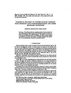
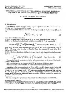
in Tables 1–3. Also, Figs. 1 and 2 show the numerical solution of u  x , t  , v (x , t ) and w (x , t ) obtained by ADM and VIM for different values of t and k . The comparison shows that the two solutions obtained are in excellent agreement. Table 1: Comparison of the approximate values of u  x ,t  obtained by ADM and VIM k=1 x t=1

t=10

ADM

k=16 VIM

ADM

VIM

0

1.18149782428374e-06 1.18149782428374e-06 1.89036297600575e-05 1.89036297600735e-05

0.02

1.06449275718299e-06 1.06449275718299e-06 1.70315819406251e-05 1.70315819406381e-05

0.04

0.111258461144262

0.111258461144262

0.111229712112651

0.111229712112652

0.06

0.311724080934518

0.311724080934518

0.311415834545380

0.311415834545650

0.08

0.450440570555619

0.450440570555619

0.449789011581172

0.449789011582907

0.1

0.499946008340295

0.499946008340295

0.499143488414013

0.499143488416931

0

1.18147823405838e-05 1.18147823405875e-05 0.000189002612493013 0.000189002612654228

0.02

1.06447510788105e-05 1.06447510788135e-05 0.000170285506268076 0.000170285506398551

0.04

0.111240409654597

0.111240409654597

0.110953967697041

0.110953967704470

0.06

0.311536827466610

0.311536827466650

0.308486109671180

0.308486112352978

0.08

0.450046187931907

0.450046187932178

0.443626629273357

0.443626646500444

0.1

0.499460613288168

0.499460613288623

0.491566313818436

0.491566342779843

Table 2: Comparison of the approximate values of v  x , t  obtained by ADM and VIM k=1

t=1

x

ADM

VIM

ADM

VIM

0

0.249999278075943

0.249999278075943

0.249990417008777

0.249990417008777

0.02

0.225241566544505

0.225241566544505

0.225233582998833

0.225233582998833

0.04

0.155873327356743

0.155873327356743

0.155887701773949

0.155887701773949

0.0556404903603832

0.0556404903603832

0.0557946135306025

0.0557946135304677

0.06

t=10

k=16

0.08

2.17526106277004e-05 2.17526106276869e-05 0.000347532165547758 0.000347532164680407

0.1

2.67970603236263e-05 2.67970603236036e-05 0.000428057131968682 0.000428057130509496

0

0.249992780853291

0.249992780853291

0.249904186818424

0.249904186818344

0.02

0.225235712749163

0.225235712749163

0.225155892263641

0.225155892263576

251

Ann J. Al-Sawoor & Mohammed O. Al-Amr 0.04

0.155881218289336

0.155881218289336

0.156024429485341

0.156024429481474

0.06

0.0557327388180641

0.0557327388180435

0.0572580953762259

0.0572580940346638

0.08 0.000217332550719252 0.000217332550584134 0.00342711857880960

0.00342710996549422

0.1

0.00421485224502687

0.000267706319170774 0.000267706318943284 0.00421486672459296

Table 3: Comparison of the approximate values of w  x , t  obtained by ADM and VIM k=1

t=1

t=10

k=16

x

ADM

VIM

ADM

VIM

0

0.249999868824855

0.249999868824855

0.249999868823657

0.249999868823657

0.02

0.225242098790883

0.225242098790883

0.225242098789804

0.225242098789804

0.04

0.211502557928874

0.211502557928875

0.211502557830275

0.211502557830275

0.06

0.211502530827642

0.211502530827642

0.211502530803293

0.211502530803293

0.08

0.225242037888437

0.225242037888437

0.225242037956134

0.225242037956134

0.1

0.249999801230471

0.249999801230471

0.249999801338975

0.249999801338975

0

0.249998688244461

0.249998688244461

0.249998688124671

0.249998688124671

0.02

0.225241035124702

0.225241035124702

0.225241035016775

0.225241035016775

0.04

0.211501423116634

0.211501423116634

0.211501413333862

0.211501413333709

0.06

0.211501152551369

0.211501152551369

0.211501150211816

0.211501150211153

0.08

0.225240426516673

0.225240426516673

0.225240433215488

0.225240433215716

0.1

0.249998012963255

0.249998012963255

0.249998023633811

0.249998023634949

252

Numerical Solution of a Reaction-Diffusion System with…

(b)

(a)

(c)

(d)

(e)

(f)

Fig.1. (a) The numerical results for u (x , t ) obtained by ADM with k  1 , (b) The numerical results for u (x , t ) obtained by VIM with k  1 , (c) The numerical results for v (x , t ) obtained by ADM with k  1 , (d) The numerical results for v (x , t ) obtained by VIM with k  1 , (e) The numerical results for w (x , t ) obtained by ADM with k  1 , (f) The numerical results for w (x , t ) obtained by VIM with k  1 .

253

Ann J. Al-Sawoor & Mohammed O. Al-Amr

(a)

(b)

(c)

(d)

(e)

(f)

Fig.2. (a) The numerical results for u (x , t ) obtained by ADM with k  16 , (b) The numerical results for u (x , t ) obtained by VIM with k  16 , (c) The numerical results for v (x , t ) obtained by ADM with k  16 , (d) The numerical results for v (x , t ) obtained by VIM with k  16 , (e) The numerical results for w (x , t ) obtained by ADM with k  16 , (f) The numerical results for w (x , t ) obtained by VIM with k  16 .

254

Numerical Solution of a Reaction-Diffusion System with…

6. Conclusions In this paper, the Adomian decomposition method (ADM) and variational iteration method (VIM) were implemented to solve reaction-diffusion system which describes a fast reversible chemical reaction. The VIM reduces the volume of calculations by not requiring the Adomian polynomials while ADM requires the use of Adomian polynomials for non-linear terms, and this needs more work. However, the results show that the two methods are very simple and effective for non-linear problems. In our work, we used Matlab codes to obtain the solutions from the two algorithms.

255

Ann J. Al-Sawoor & Mohammed O. Al-Amr

REFERENCES [1] [2] [3] [4] [5]

[6]

[7]

[8] [9]

[10] [11]

[12] [13]

[14] [15] [16] [17]

Abdou, M.A. and Soliman, A.A., (2005), “New applications of variational iteration method”, Physica D, 211, 1–8. Adomian, G., (1984), “A new approach to nonlinear partial differential equations”, J. Math. Anal. Appl., 102, 420–434. Adomian, G., (1988), “A review of the decomposition method in applied mathematics”, J. Math. Anal. Appl. 135, 501–544. Adomian, G., (1994), “Solving frontier problems of physics: the decomposition method”, Kluwer Acad. Publ. Afrouzi, G.A. and Khademloo, S., (2006), “On Adomian Decomposition Method for Solving Reaction Diffusion Equation”, Int. J. Nonlinear Sci., 2(1), 11-15. Alabdullatif, M., Abdusalam, H. A. and Fahmy, E.S., (2007), “Adomian decomposition method for nonlinear reaction diffusion system of Lotka-Volterra type”, International Mathematical Forum, 2(2), 87-96. Batiha, B., Noorani, M.S.M., Hashim, I. and Batiha, K., (2008), “Numerical simulations of systems of PDEs by variational iteration method”, Physics Letters A, 372, 822–829. Bothe, D. and Hilhorst, D., (2003), “A reaction–diffusion system with fast reversible reaction”, J. Math. Anal. Appl., 268(1), 125–135. El-Sayed, A.M.A., Rida, S.Z. and Arafa, A.A.M., (2010), “On the Solutions of the Generalized Reaction-Diffusion Model for Bacterial Colony”, Acta Appl. Math., 110, 1501–1511. El-Wakil, S.A. and Abdou, M.A., (2007), “New applications of Adomian decomposition method”, Chaos Solitons Fractals, 33, 513–522. Érdi, P. and Tóth, J., (1989), “Mathematical models of chemical reactions, Nonlinear Science: Theory and Applications”, Princeton University Press, Princeton, NJ. Espenson, J. H., (1995), “Chemical Kinetics and Reaction Mechanisms”, Mc Graw-Hill, New York. Eymard, R., Hilhorst, D., Murakawa, H., and Olech, M., (2010), “Numerical Approximation of a Reaction-Diffusion System with Fast Reversible Reaction”, Chin. Ann. Math., 31B(5), 631–654. He, J.H. and Wu, X.H., (2007), “Variational iteration method: New development and applications”, Comput. Math. Appl., 54, 881–894. He, J.H., (1997), “A new approach to nonlinear partial differential equations”, Comm. Nonlinear Sci. Numer. Simul., 2 (4), 203–205. He, J.H., (1999). “Variational iteration method–a kind of non-linear analytical technique: Some examples”, Int. J. Nonlinear. Mech., 34, 699-708. He, J.H., (2007), “Variational iteration method–Some recent results and new interpretations”, J. Comput. Appl. Math., 207, 3–17.

256

Numerical Solution of a Reaction-Diffusion System with…

[18]

[19]

[20] [21]

[22]

[23]

[24] [25] [26]

[27]

Jalilian, Y., (2008), “A Variational Iteration Method for Solving Systems of Partial Differential Equations and for Numerical Simulation of the Reaction– Diffusion Brusselator Model”, Scientia Iranica, 15(2), 223–229. Meyer, H., Klein, J., and Weiss, A., (1979), “Kinetische untersuchung der reversiblen dimerisierung von o-phenylendioxidimethylsilan”, J. Organometallic Chem., 177, 323–328. Pamuk, S., (2005), “An application for linear and nonlinear heat equations by Adomian’s decomposition method”, Appl. Math. Comput., 163 , 89–96. Raslan, K.R., Soliman, A.A. and Ali, A.H.A., (2012), “A comparison between the variational iteration method and Adomian decomposition method for the FitzHugh- Nagumo equations”, Int. J. Phys. Sci., 7(15), 2302 – 2309. Soliman, A.A. and Abdou, M.A., (2007), “Numerical solutions of nonlinear evolution equations using variational iteration method”, J. Comput. Appl. Math., 207, 111–120. Wazwaz, A., (2000), “The decomposition method applied to systems of partial differential equations and to the reaction-diffusion Brusselator model”, Appl. Math. Comput., 110, 251-264. Wazwaz, A., (2007), “A Comparison between the variational iteration method and Adomian decomposition method”, J. Comput. Appl. Math., 207(1), 129-136. Wazwaz, A., (2007), “The variational iteration method for solving linear and nonlinear systems of PDEs”, Comput. Math. Appl., 54, 895–902. Wazwaz, A., (2007), “The variational iteration method: A powerful scheme for handling linear and nonlinear diffusion equations”, Comput. Math. Appl., 54, 933–939. Wilhelmsson, H., (1988), “Simultaneous diffusion and reaction processes in plasma dynamics”, Phys. Rev. A, 38, 1482–1489.

257