Numerical solution of a two-dimensional IHCP based

Journal of Advanced Research in Applied Mathematics Online ISSN: 1942-9649

Vol. , Issue. , 2012, pp. 1-16 doi: 10.5373/jaram.

Numerical solution of a two-dimensional IHCP based on Duhamel’s principle Reza Pourgholi∗ , Amin Esfahani, Akram Saeedi School of Mathematics and Computer Sciences, Damghan University, Damghan, Iran.

Abstract. In this paper, we will first study the existence and uniqueness of the solution for a two-dimensional inverse heat conduction problem (IHCP). Furthermore, the estimate of an unknown boundary condition by a numerical algorithm in this IHCP based on Duhamel’s principle, is the topic of this paper. The stability and accuracy of the scheme presented is evaluated by comparison with the Singular Value Decomposition method. Some numerical experiments confirm the utility of this algorithm as the results are in good agreement with the exact data. Keywords: Inverse heat conduction problem; Existence and uniqueness; Duhamel’s principle, SVD method. Mathematics Subject Classification 2010: 65M32, 35K05.

1

Introduction

Inverse heat conduction problems (IHCPs) have been extensively studied over the last 60 years. They have numerous applications in many branches of science and technology. The problem consists in determining the temperature and flux heat at inaccessible parts of the boundary of a 2 or 3-dimensional body from corresponding data on accessible parts of the boundary. It is well-known that IHCPs are severely ill-posed which means that small perturbations in the data may cause extremely large errors in the solution. Fortunately, many methods have been reported to solve IHCPs ( [1]- [3]), [6], [7], [16], [26], ( [30]- [36]) , and among the most versatile methods the following can be mentioned: Tikhonov regularization [37], iterative regularization [1], mollification [24], base function method (BFM) [31], semi finite difference method (SFDM) [26], and the

∗

Correspondence to: R. Pourgholi, School of Mathematics and Computer Science, Damghan University, Damghan, Iran. Email: [email protected] † Received: 1 February 2012, accepted: 27 May 2012. http://www.i-asr.com/Journals/jaram/

1

c ⃝2012 Institute of Advanced Scientific Research

2

Numerical solution of a two-dimensional IHCP based on Duhamel’s principle

function specification method (FSM) [2]. Dowding and Beck [7] addressed a sequential gradient method for two dimensional IHCPs with and without function specification, additionally using the conventional regularization method. Kim et al. [36] solved an inverse heat conduction problem to estimate the surface temperature from temperature readings. Su and Neto [35] solved a two-dimensional inverse heat conduction problem to estimate the radial and circumferential transient dependence of the strength of a volumetric heat source in a cylindrical rod. Huang and Tsai [16] solved a three-dimensional inverse heat conduction problem to estimate the local time-dependent surface heat transfer coefficients for plate finned-tube heat exchangers. However, only few works have been done on the two-dimensional problems because of the complicated interaction and reflection of the thermal wave [5,6], [5]. Yang Ching-yu, [6] developed the two-dimensional hyperbolic heat conduction equations in an arbitrary body-fitted coordinate grid and used non-oscillatory numerical schemes to approach the problem. Chen and Lin [5, 6] formulated a numerical scheme involving the Laplace transform technique and the control volume method for the problem. In this paper, a numerical method consisting of Tikhonov regularization 0th, 1st and 2nd to the matrix form of Duhamel’s principle for solving this inverse problem using measurement data containing noise is presented. This algorithm is capable of estimating the temperature in surface in space and time-varying. The measurements ensure that the inverse problem has a unique solution, but this solution is unstable hence the problem is ill-posed. This instability is overcome using the zeroth-, first-, and second-order Tikhonov regularization method with the GCV criterion for the choice of the regularization parameter. The stability and accuracy of the scheme presented is evaluated by comparison with the Singular Value Decomposition method (SVD). Numerical results show that an excellent estimation can be obtained within a couple of minutes CPU time at pentium(R) 4 CPU 3.20 GHz.

2

Problem statement

The inverse problem is to find one part of the boundary conditions in two-dimensional body while the temperature measurements at the other part are given. For Q = {(x, y, t) : x ∈ (0, 1), y ∈ (0, 1), t ∈ (0, tM )}, the dimensionless mathematical formulation of two-dimensional IHCP may be expressed as follows: Tt (x, y, t) = Txx (x, y, t) + Tyy (x, y, t),

in Q,

(2.1a)

T (0, y, t) = q(y, t),

0 ≤ y ≤ 1, 0 ≤ t ≤ tM ,

(2.1b)

T (1, y, t) = µ(y, t),

0 ≤ y ≤ 1, 0 ≤ t ≤ tM ,

(2.1c)

T (x, 0, t) = ψ(x, t),

0 ≤ x ≤ 1, 0 ≤ t ≤ tM ,

(2.1d)

T (x, 1, t) = p(x, t),

0 ≤ x ≤ 1, 0 ≤ t ≤ tM ,

(2.1e)

T (x, y, 0) = h(x, y),

0 ≤ x ≤ 1, 0 ≤ y ≤ 1,

(2.1f)

Reza Pourgholi, Amin Esfahani and Akram Saeedi

3

and, for a fixed point (x1 , y1 ) where 0 < x1 < 1 and 0 < y1 < 1, the overspecified condition T (x1 , y1 , t) = g(x1 , y1 , t),

0 ≤ t ≤ tM ,

(2.1g)

where µ(y, t), ψ(x, t), p(x, t) and h(x, y) are known functions and tM represents the final time of interest for the time evolution of the problem while q(y, t) is unknown. Equations of the type of (2.1) are used to model phenomena occurring in various fields: chemistry, biology, neurophysiology, epidemiology, combustion, population genetics, ecology, geology, etc.; see for example [4, 10, 11, 18] and its numerous references. The solutions of reactiondiffusion equations display a wide range of behaviors, including the formation of traveling waves and selforganized patterns. Diffusion equations play a central role in probability (Brownian motion, Markov processes, diffusion processes, stochastic differential equations, etc.); see for example [34]. An interesting use of the heat equation has been made in connection with the Atiyah-Singer index; see for example [12]. Before describing our numerical method for solving (2.1), we would like to recall some results regarding existence and uniqueness of solution of problem (2.1a)-(2.1f) assuming that q is given. We should note that by a change of variable, we can consider the following equivalent form of problem (2.1a)-(2.1g),  (x, y) ∈ Ω = (0, 1) × (0, 1), t > 0,   ut = uxx + uyy ,  e u(x, y, 0) = h(x, y), (x, y) ∈ Ω, (2.2)  u(0, y, t) = u(1, y, t) = 0, y ∈ [0, 1], t ≥ 0,   u(x, 0, t) = u(x, 1, t) = 0, x ∈ [0, 1], t ≥ 0, where here e h depends on p, ψ, h, µ and q. Now we apply the Hille-Yosida theory in L2 (Ω) (see [29]). Theorem 2.1. Let e h ∈ L2 (Ω). Then there exists a unique solution u(x, y, t) of (2.2) such that ( ) ( ) u ∈ C [0, +∞); L2 (Ω) ∩ C (0, +∞); H 2 (Ω) ∩ H01 (Ω) , (2.3) where H 2 (Ω) and H01 (Ω) are the usual Sobolev spaces. Moreover, ( ) ( ) u ∈ C 1 (0, +∞); L2 (Ω) ∩ L2 (0, +∞); H01 (Ω) . Furthermore, u satisfies

( ) u ∈ C ∞ Ω × [ε, +∞) ,

(2.4)

for all ε > 0. Proof. Consider the unbounded operator A : D(A) ⊂ L2 (Ω) → L2 (Ω) defined by A = −∂x2 − ∂y2 , where D(A) = H 2 (Ω) ∩ H01 (Ω). It is straightforward to check that A is a self-adjoint maximal monotone operator. We may then apply the Hille-Yosida theorem [20–23, 29, 41] and deduce the existence of a unique solution of (2.2) satisfying (2.3) and (2.4).

4

Numerical solution of a two-dimensional IHCP based on Duhamel’s principle

If we make additional assumptions on e h the solution u becomes more regular up to t = 0. Theorem 2.2. If e h ∈ H01 (Ω), then the solution u of (2.2) satisfies ( ) u ∈ C [0, +∞); H01 (Ω) ∩ L2 ((0, +∞); H 2 (Ω)). Proof. We work in the space H01 (Ω) equipped with the scalar product ∫ 1∫ 1 ⟨u, v⟩ = uv + ux vx + uy vy dx dy. 0

0

Consider the unbounded operator A : D(A) ⊂ H01 (Ω) → H01 (Ω), where A is defined as in the proof of Theorem 2.1 and { } D(A) = u ∈ H 3 (Ω) ∩ H01 (Ω); −Au ∈ H01 (Ω) . One can observe from the definition and the regularity argument for the Dirichlet problem that the operator A is maximal monotone and self-adjoint. Applying again the Hille-Yoside theorem, we see that if e h ∈ H01 (Ω) there exists a solution u of (2.2), which coincides with the one obtained in Theorem 2.1 because of uniqueness, such that u ∈ C([0, +∞); H01 (Ω)).

Remark 2.3. We should note that system (2.2) can be also solved by a decomposition in a Hilbert basis of L2 (Ω). Indeed, it is very convenient to choose a basis {ej }j of L2 (Ω) composed of eigenfunctions of A = −∂x2 − ∂y2 , with zero Dirichlet condition, i.e., {

Aej = λ2j ej , ej = 0,

in Ω, in ∂Ω.

Suppose that e h ∈ L2 (Ω). We seek a solution u of (2.2) in the form of a series u(x, y, t) =

∞ ∑

aj (t) ej (x, y).

j=1

We see immediately that the functions aj (t) must satisfy a′j (t) + λ2j aj (t) = 0, so that aj (t) = cj exp(−λ2j t). The constants cj are determined by the relation e h(x, y) =

∞ ∑ j=1

cj ej (x, y).

(2.5)

Reza Pourgholi, Amin Esfahani and Akram Saeedi

5

In other words, the solution u of (2.2) is given by u(x, y, t) =

∞ ∑

cj e−λj t ej (x, y). 2

j=1

where the constants cj are the components of h in the basis {ej }, i.e., ∫ 1∫ 1 cj = h(x, y) ej (x, y) dx dy. 0

0

For the study of the convergence of this series (and also the regularity of u obtained in this way) we refer to [40]. Assuming q is given, so Theorems 2.1, 2.2 and Remark 2.3 guarantees the existence of a unique solution T = T (x, y, t; q) of (2.1). Now, condition (2.1g) determines q uniquely.

3

Description of method

The solution of the problem (2.1) can be written as follows T (x, y, t) =

5 ∑

Ti (x, y, t),

i=1

where Ti (x, y, t), for i = 1, 2, 3, 4, 5, satisfy the following problem: ∂Ti ∂ 2 Ti ∂ 2 Ti = + , ∂t ∂x2 ∂y 2 { q(y, t), i = 1 Ti (0, y, t) = 0, otherwise { µ(y, t), i = 2 Ti (1, y, t) = 0, otherwise { ψ(x, t), i = 3 Ti (x, 0, t) = 0, otherwise { p(x, t), i = 4 Ti (x, 1, t) = 0, otherwise { h(x, y), i = 5 Ti (x, y, 0) = 0, otherwise

in Q,

(3.1a)

0 ≤ y ≤ 1, 0 ≤ t ≤ tM ,

(3.1b)

0 ≤ y ≤ 1, 0 ≤ t ≤ tM ,

(3.1c)

0 ≤ x ≤ 1, 0 ≤ t ≤ tM ,

(3.1d)

0 ≤ x ≤ 1, 0 ≤ t ≤ tM ,

(3.1e)

0 ≤ x ≤ 1, 0 ≤ y ≤ 1.

(3.1f)

In a linear problem a linear dependence exists between the input (in this case q(y, t)) and the response (at x = 1). This dependence can be expressed analytically by the Duhamel integral [2] ∫ t ∂ϕ T1 (x, y, t) = q(s) (x, y, t − s)ds + T1 (x, y, 0), (3.2) ∂t 0

6

Numerical solution of a two-dimensional IHCP based on Duhamel’s principle

where ϕ(x, y, t) represents the temperature response at location (x, y) for a unit step change in the input, and T1 (x, y, 0) is the initial condition for problem (3.1) for i = 1 (in this case it is 0). Considering that the objective in the inverse problem (3.1), for i = 1, is the estimate of q(y, t) in a discrete form equation (3.2) can be approximated at time tM as (T1 )M =

M ∑

qn ∆ϕM −n ,

(3.3)

n=1

where qn the measured temperature at time tn , Note that ∆ϕ represents the temperature response to a unit pulse in the input so that ∆ϕk = ϕk+1 − ϕk for k = 1, ..., M . Note 1k that ∆ϕk−j = ∂T ∂qj , therefore, it represents the sensitivity coefficient measured at time tk with respect to component qj . Obviously, the sensitivity coefficients will be zero when k < j. Writing the equation (3.3), for M = 1, 2, . . . points, consequently, we obtain the following matrix equation T1 = Xq (3.4) where q = [q1 , . . . , qM ]T , qk = q(tk ) and   ∆ϕ0 0 ... 0 0 0  ∆ϕ1 ∆ϕ0 0 ... 0 0     .. .. .. .. .. ..  . X= . . . . . .    ∆ϕM −2 ∆ϕM −3 ... ∆ϕ1 ∆ϕ0 0  ∆ϕM −1 ∆ϕM −2 ∆ϕM −3 . . . ∆ϕ1 ∆ϕ0 If the time history covers a large period of time, this matrix and the corresponding vector can be of a considerable dimensional. By solving the direct problem (3.1), for i = 2, 3, 4, 5, and using the overspecified condition (2.1g) and the equation (2.1), we have ∗

T (x1 , y1 , t) = g(x1 , y1 , t) −

5 ∑

Ti (x1 , y1 , t) = T1 (x1 , y1 , t).

(3.5)

i=2

Considering Duhamel’s Theorem, for M = 1, 2, . . ., we obtain the following equation T ∗ = Xq,

(3.6)

∗ ]T , T ∗ = T ∗ (x , y , t ). where T ∗ = [T1∗ , . . . , TM 1 1 k k In this study we consider a possible method in order to get a stable algorithm, so that the Tikhonov regularization method must be used to control this measurement errors. The Tikhonov regularized solution ( [38], [14] and [19]) to the system of linear algebraic equation (3.6) is given by

zα (q) = ∥Xq − T ∗ ∥22 + α∥R(s) q∥22 .

Reza Pourgholi, Amin Esfahani and Akram Saeedi

7

On the case of the zeroth-, first-, and second-order Tikhonov regularization method the matrix R(s) , for s = 0, 1, 2, is given by, see e.g. [25]: R(0) = IM ×M ∈ RM ×M ,   −1 1 . . . 0 0 0  0 −1 1 . . . 0 0    .. .. .. .. ..  ∈ R(M −1)×M , R(1) =  ... . . . . .   0 0 . . . −1 1 0 0 0 . . . 0 −1 1   1 −2 1 0 . . . 0 0 0 1 −2 1 0 . . . 0    .. .. .. .. .. ..  ∈ R(M −2)×M . R(2) =  ... . . . . . .   0 0 . . . 1 −2 1 0 0 0 . . . 0 1 −2 1 Therefore, we obtain the Tikhonov regularized solution of the regularized equation as [ ]−1 qα = X T X + α(R(s) )T R(s) X T T ∗ . In our computation, we use the GCV scheme to determine a suitable value of α ( [9], [13] and [39]). Remark 3.1. In an IHCP there are two sources of error in the estimation. The first source is the unavoidable bias deviation (or deterministic error). The second source of error is the variance due to the amplification of measurement errors (stochastic error). The global effect of deterministic and stochastic errors is considered in the mean squared error or total error, [3]. Therefore, we compare Tikhonov regularization 0th, 1st and 2nd method and SVD method by considering total error S defined by [ S=

]1 1 ∑ 2 (qbi − qi )2 , N −1 N

(3.7)

i=1

where N is the total number of estimated values.

4

Numerical results and discussion

In this section, we demonstrate numerically some of results for the unknown boundary condition in the inverse problem (2.1). The propose of this section is to illustrate the applicability of the present method described in Section 3 for solving IHCP. As expected, the IHCP is ill-posed and therefore it is necessary to investigate the stability of the present method by giving a test problem.

8

Numerical solution of a two-dimensional IHCP based on Duhamel’s principle

Example 4.1. In this example, let us consider the following two-dimensional inverse problem, for estimating unknown boundary condition q(y1 , t) when x1 = 0.2 and y1 = 0.6. Tt (x, y, t) = Txx (x, y, t) + Tyy (x, y, t),

in Q,

(4.1a)

T (0, y, t) = q(y, t),

0 ≤ y ≤ 1, 0 ≤ t ≤ 2,

(4.1b)

−t

0 ≤ y ≤ 1, 0 ≤ t ≤ 2,

(4.1c)

−t

0 ≤ x ≤ 1, 0 ≤ t ≤ 2,

(4.1d)

−t

T (x, 1, t) = e (sin x + cos 1),

0 ≤ x ≤ 1, 0 ≤ t ≤ 2,

(4.1e)

T (x, y, 0) = sin x + cos y,

0 ≤ x ≤ 1, 0 ≤ y ≤ 1,

(4.1f)

0 ≤ t ≤ 2.

(4.1g)

T (1, y, t) = e (sin 1 + cos y), T (x, 0, t) = e (sin x + 1),

and the overspecified condition T (0.2, 0.6, t) = e−t (sin 0.2 + cos 0.6), The exact solution of this problem is T (x, y, t) = e−t sin x + e−t cos y

and q(y, t) = e−t cos y.

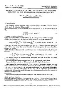
Table 1 show the comparison between the exact solution and approximate solutions result using Tikhonov regularization and SVD method with noiseless data, and Table 2 and figure 1 show the comparison between the exact solution and approximate solutions result with noise data. At the end, we compare the methods by computing the total error (3.7). t 0.08 0.32 0.56 0.80 1.04 1.28 1.52 1.76 2.00

Exact 0.761881 0.599317 0.471439 0.370847 0.291719 0.229474 0.180511 0.141995 0.111697 S

Tikhonov 0th 0.407866 0.303368 0.238491 0.187603 0.147574 0.116085 0.091316 0.071830 0.056222 1.945e − 001

Tikhonov 1st 0.803756 0.595018 0.468075 0.368197 0.289634 0.227834 0.179221 0.140980 0.110857 8.98e − 003

Tikhonov 2nd 0.786855 0.596801 0.468805 0.368768 0.290084 0.228188 0.179499 0.141205 0.112819 5.61e − 003

SVD 0.805548 0.595416 0.468074 0.368198 0.289635 0.227835 0.179221 0.140980 0.110899 9.24e − 003

Table 1. The comparison between exact, Tikhonov 0th and Tikhonov 1st, Tikhonov 2nd and SVD solutions for q(0.6, t) with noiseless data when ∆t = 0.08.

Reza Pourgholi, Amin Esfahani and Akram Saeedi

t 0.08 0.32 0.56 0.80 1.04 1.28 1.52 1.76 2.00

Exact 0.761881 0.599317 0.471439 0.370847 0.291719 0.229474 0.180511 0.141995 0.111697 S

Tikhonov 0th 0.409337 0.304830 0.239954 0.189065 0.149036 0.117548 0.092778 0.073292 0.057677 1.958e − 001

Tikhonov 1st 0.806658 0.597888 0.470945 0.371067 0.292504 0.230704 0.182091 0.143850 0.113727 9.45e − 003

Tikhonov 2nd 0.789753 0.599672 0.471676 0.371639 0.292954 0.231058 0.182369 0.144076 0.115689 6.33e − 003

9

SVD 0.808450 0.598287 0.470944 0.371068 0.292505 0.230705 0.182091 0.143851 0.113769 9.70e − 003

Table 2. The comparison between exact, Tikhonov 0th, Tikhonov 1st, Tikhonov 2nd and SVD solutions for q(0.6, t) with discrete noisy data when ∆t = 0.08. 0.9 SVD Tikhonov 0th Tikhonov 1st Tikhonov 2nd Exact

0.8 0.7

q(0.6,t)

0.6 0.5 0.4 0.3 0.2 0.1 0

0

0.2

0.4

0.6

0.8

1 t

1.2

1.4

1.6

1.8

2

Figure 1. The comparison between the exact results and the present numerical results of the problem (4.1) with discrete noisy data when ∆t = 0.08. 0

−0.05

−0.1

Error

−0.15

−0.2

−0.25

−0.3

−0.35

−0.4

line 0 qTikhonov 0th(0.6,t)−qExact(0.6,t) 0

0.2

0.4

0.6

0.8

1 t

1.2

1.4

1.6

1.8

2

Figure 2. Difference between the q(0.6, t)exact , q(0.6, t)T ikhonov 0th of the problem (4.1) with discrete noisy data when ∆t = 0.08.

10

Numerical solution of a two-dimensional IHCP based on Duhamel’s principle

0.03

0.025

0.02 line 0 qTikhonov 1st(0.6,t)−qExact(0.6,t)

Error

0.015

0.01

0.005

0

−0.005

0

0.2

0.4

0.6

0.8

1 t

1.2

1.4

1.6

1.8

2

Figure 3. Difference between the q(0.6, t)exact , q(0.6, t)T ikhonov 1st of the problem (4.1) with discrete noisy data when ∆t = 0.08. 0.045 0.04 0.035 0.03 line 0 qTikhonov 2nd(0.6,t)−qExact(0.6,t)

Error

0.025 0.02 0.015 0.01 0.005 0 −0.005

0

0.2

0.4

0.6

0.8

1 t

1.2

1.4

1.6

1.8

2

Figure 4. Difference between the q(0.6, t)exact , q(0.6, t)T ikhonov 2nd of the problem (4.1) with discrete noisy data when ∆t = 0.08. 0.05

0.04 line 0 qSVD(0.6,t)−qExact(0.6,t)

Error

0.03

0.02

0.01

0

−0.01

0

0.2

0.4

0.6

0.8

1 t

1.2

1.4

1.6

1.8

2

Figure 5. Difference between the q(0.6, t)exact , q(0.6, t)SV D of the problem (4.1) with discrete noisy data when ∆t = 0.08.

Reza Pourgholi, Amin Esfahani and Akram Saeedi

11

Example 4.2. Now, we consider the following two-dimensional inverse problem for estimating unknown boundary condition ψ(x1 , t) when x1 = 0.8, y1 = 0.1. Tt (x, y, t) = Txx (x, y, t) + Tyy (x, y, t),

in Q,

(4.2a)

0 ≤ y ≤ 1, 0 ≤ t ≤ 1,

(4.2b)

T (1, y, t) = e (sin 1 + sin y),

0 ≤ y ≤ 1, 0 ≤ t ≤ 1,

(4.2c)

T (x, 0, t) = ψ(x, t),

0 ≤ x ≤ 1, 0 ≤ t ≤ 1,

(4.2d)

T (x, 1, t) = e (sin x + sin 1),

0 ≤ x ≤ 1, 0 ≤ t ≤ 1,

(4.2e)

T (x, y, 0) = sin x + sin y,

0 ≤ x ≤ 1, 0 ≤ y ≤ 1,

(4.2f)

0 ≤ t ≤ 1.

(4.2g)

−t

T (0, y, t) = e

sin y,

−t

−t

and the overspecified condition T (0.8, 0.1, t) = e−t (sin 0.8 + sin 0.1), The exact solution of this problem is T (x, y, t) = e−t (sin x + sin y) and ψ(x, t) = e−t sin x. Table 3 show the comparison between the exact solution and approximate solutions result using Tikhonov regularization and SVD method with noiseless data, and Table 4 and figure 6 show the comparison between the exact solution and approximate solutions result with noise data. At the end, we compare the methods by computing the total error (3.7).

t 0.04 0.16 0.28 0.40 0.52 0.64 0.76 0.88 1.00

Exact 0.689228 0.611291 0.542166 0.480858 0.426483 0.378256 0.335483 0.297547 0.263901 S

Tikhonov 0th 0.355167 0.315491 0.279866 0.248223 0.220154 0.195259 0.173173 0.153527 0.135011 2.253e − 001

Tikhonov 1st 0.696597 0.613116 0.543596 0.482108 0.427589 0.379238 0.336354 0.298319 0.264561 2.05e − 003

Tikhonov 2nd 0.690598 0.613440 0.543808 0.482291 0.427751 0.379381 0.336481 0.298436 0.266798 1.64e − 003

SVD 0.704518 0.621737 0.546182 0.491093 0.436501 0.380444 0.343713 0.298525 0.270855 2.066e − 003

Table 3. The comparison between exact, Tikhonov 0th, Tikhonov 1st, Tikhonov 2nd and SVD solutions for ψ(0.8, t) with noiseless data when ∆t = 0.04.

12

Numerical solution of a two-dimensional IHCP based on Duhamel’s principle

t 0.04 0.16 0.28 0.40 0.52 0.64 0.76 0.88 1.00

Exact 0.689228 0.611291 0.542166 0.480858 0.426483 0.378256 0.335483 0.297547 0.263901 S

Tikhonov 0th 0.359095 0.319864 0.281213 0.252816 0.224716 0.195928 0.176962 0.153700 0.138215 2.283e − 001

Tikhonov 1st 0.698261 0.620589 0.546718 0.490239 0.435932 0.381948 0.344046 0.300700 0.273436 7.904e − 003

Tikhonov 2nd 0.681569 0.618917 0.547837 0.488637 0.424207 0.384367 0.342960 0.304251 0.261073 7.735e − 003

SVD 0.704518 0.621737 0.546182 0.491093 0.436501 0.380444 0.343713 0.298525 0.270855 8.3716e − 003

Table 4. The comparison between exact, Tikhonov 0th, Tikhonov 1st, Tikhonov 2nd and SVD solutions for ψ(0.8, t) with discrete noisy data when ∆t = 0.04. 0.8 SVD Tikhonov 0th Tikhonov 1st Tikhonov 2nd Exact

0.7

ψ(0.8,t)

0.6

0.5

0.4

0.3

0.2

0.1

0

0.1

0.2

0.3

0.4

0.5 t

0.6

0.7

0.8

0.9

1

Figure 6. The comparison between the exact results and the present numerical results of the problem (4.2) with discrete noisy data when ∆t = 0.04. 0

−0.05 line 0 ψTikhonov 0th(0.8,t)−ψExact(0.8,t)

−0.1

Error

−0.15

−0.2

−0.25

−0.3

−0.35

0

0.1

0.2

0.3

0.4

0.5 t

0.6

0.7

0.8

0.9

1

Figure 7. Difference between the ψ(0.8, t)exact , ψ(0.8, t)T ikhonov 0th of the problem (4.2) with discrete noisy data when ∆t = 0.04.

Reza Pourgholi, Amin Esfahani and Akram Saeedi

13

0.012 line 0 ψTikhonov 1st(0.8,t)−ψExact(0.8,t) 0.01

Error

0.008

0.006

0.004

0.002

0

0

0.1

0.2

0.3

0.4

0.5 t

0.6

0.7

0.8

0.9

1

Figure 8. Difference between the ψ(0.8, t)exact , ψ(0.8, t)T ikhonov 1st of the problem (4.2) with discrete noisy data when ∆t = 0.04. 0.014 line 0 ψTikhonov 2nd(0.8,t)−ψExact(0.8,t)

0.012

0.01

Error

0.008

0.006

0.004

0.002

0

0

0.1

0.2

0.3

0.4

0.5 t

0.6

0.7

0.8

0.9

1

Figure 9. Difference between the ψ(0.8, t)exact , ψ(0.8, t)T ikhonov 2nd of the problem (4.2) with discrete noisy data when ∆t = 0.04. 0.016

0.014 line 0 ψSVD(0.8,t)−ψExact(0.8,t)

0.012

Error

0.01

0.008

0.006

0.004

0.002

0

0

0.1

0.2

0.3

0.4

0.5 t

0.6

0.7

0.8

0.9

1

Figure 10. Difference between the ψ(0.8, t)exact , ψ(0.8, t)SV D of the problem (4.2) with discrete noisy data when ∆t = 0.04.

14

5

Numerical solution of a two-dimensional IHCP based on Duhamel’s principle

Conclusion

A numerical method to estimate unknown boundary condition is proposed for these kinds of IHCPs and the following results are obtained: 1. The present study successfully applies the numerical method to IHCPs. 2. Numerical results show that a good estimation can be obtained within a couple of minutes CPU time at Pentium(R) 4 CPU 3.2 GHz. 3. Our calculations show that our method by Tikhonov regularization, in comparison to SVD, provides a fast and efficient method for solving IHCPs in two-dimensions. 4. The stability analysis ensures that the method is stable. References [1] O.M. Alifanov. Inverse Heat Transfer Problems. Springer, NewYork, 1994. [2] J.V. Beck, B. Blackwell, C. R. St. Clair. Inverse Heat Conduction: Ill-Posed Problems. Wiley-Interscience, NewYork, 1985. [3] J.M.G. Cabeza, J.A.M. Garcia, A.C. Rodriguez. A Sequential Algorithm of Inverse Heat Conduction Problems Using Singular Value Decomposition. International Journal of Thermal Sciences, 2005, 44: 235 - 244. [4] J.R. Cannon. The One-Dimensional Heat Equation. Addison Wesley, Reading, MA, 1984. [5] H.T. Chen, J.Y. Lin. Analysis of two-dimensional hyperbolic heat conduction problems. Int. J. Heat Mass Transfer, 1994, 37: 153 - 164. [6] Y. Ching-yu. Direct and inverse solutions of the two-dimensional hyperbolic heat conduction problems. Applied Mathematical Modelling, 2009, 33: 2907 - 2918, doi: 10.1016/j.apm.2008.10.001. [7] K.J. Dowding, J.V. Beck. A Sequential Gradient Method for the Inverse Heat Conduction Problems. J. Heat Transfer, 1999, 121: 300 - 306. [8] L.M. Delves, J.L. Mohamed. Computational Methods for Integral equations. Cambridge University press, Cambridge, New York, 1985. [9] L. Elden. A Note on the Computation of the Generalized Cross-validation Function for Ill-conditioned Least Squares Problems. BIT, 1984, 24: 467 - 472. [10] P. Fife. Mathematical aspects of reacting and diffusing systems. Lecture Notes in Biomathematics, 28, Springer, 1979. [11] G.B. Folland. Introduction to Partial Differential Equations. Princeton University Press, 1976. [12] P. Gilkey. The Index theorem and the Heat Equation. Math. Lect. Series 4, 1974. [13] G.H. Golub, M. Heath, G. Wahba. Generalized Cross-validation as a Method for Choosing a Good Ridge Parameter. Technometrics, 1979, 21: 215 - 223. [14] P.C. Hansen. Analysis of discrete ill-posed problems by means of the L-curve. SIAM Rev., 1992, 34: 561 - 80. [15] F.D. Hoog, R. Weiss. On the solution of Volterra integral equations of the first kind. Numer. Math., 1973, 21: 22 - 32. [16] C.H. Huang, Y.-L. Tsai. A transient 3-D inverse problem in imaging the time-dependent local heat transfer coefficients for plate fin. Applied Thermal Engineering, 2005, 25: 2478 2495, doi: 10.1016/j.applthermaleng.2004.12.003.

Reza Pourgholi, Amin Esfahani and Akram Saeedi

15

[17] A.J. Jerri. Introduction to Integral Equations with Applications. JOHN-WILLY & Sons, INC., New York, 1999. [18] F. John. Partial Differential Equations. Springer-Verlag, New York, 1982. [19] C.L. Lawson, R.J. Hanson. Solving Least Squares Problems. Philadelphia, PA: SIAM, 1995. First published by Prentice-Hall, 1974. [20] J.-C. Lions, E. Magenes. Remarques sur les probl`emes aux limites pour op´erateurs paraboliques. Compt. Rend. Acad. Sci. (Paris), 1960, 251: 2118 - 2120. [21] J.-C. Lions, E. Magenes. Probl`emes aux limites non homog`enes. II. Annales de l’institut Fourier, 1961, 11: 137 - 178. [22] J.-C. Lions, E. Magenes. Probl`emes aux limites non homog`enes. IV. Annali della Scuola Normale Superiore di Pisa 15 (1961) 311 - 326. [23] J.-C. Lions, E. Magenes. Probl`emes aux limites non homog`enes el applications. Dunod, 1968. [24] D.A. Murio. The Mollification Method and the Numerical Solution of Ill-Posed Problems. Wiley-Interscience, NewYork, 1993. [25] L. Martin, L. Elliott, P.J. Heggs, D.B. Ingham, D. Lesnic, X. Wen. Dual Reciprocity Boundary Element Method Solution of the Cauchy Problem for Helmholtz-type Equations with Variable Coefficients. Journal of Sound and Vibration, 2006, 297: 89 - 105. [26] H. Molhem, R. Pourgholi. A numerical algorithm for solving a one-dimensional inverse heat conduction problem. Journal of Mathematics and Statistics, 2008, 4: 60 - 63. [27] N.A. Sidorov, M.V. Falaleev, D.N. Sidorov. Generalized solutions of Volterra integral equations of the first kind. Bull. Malays. Math. Sci. Soc., 2006, 29: 101 - 109. [28] M.N. Ozisik. Heat Conduction. John Wiley & Sons, Inc., New York, 1993. [29] A. Pazy. Semigroups of Linear Operators and Applications to Partial Differential Equations. Applied Mathematical Sciences, 44, Springer-Verlag, New York, 1983. [30] R. Pourgholi, N. Azizi, Y.S. Gasimov, F. Aliev, H.K. Khalafi. Removal of numerical instability in the solution of an inverse heat conduction problem. Communications in Nonlinear Science and Numerical Simulation, 2009, 14: 2664 - 2669, doi: 10.1016/j.cnsns.2008.08.002. [31] R. Pourgholi, M. Rostamian. A numerical technique for solving IHCPs using Tikhonov regularization method. Appl. Math. Modell., 2009, 4: 290 - 298, doi: 10.1016/j.apm.2009.10.022. [32] R. Pourgholi, F. Torabi, S.H. Tabasi. A numerical solution of two dimensional IHCPs by using ADI method and Tikhonov regularization method. Journal of Advanced Research in Scientific Computing, 2011, 3: 55 - 68. [33] A. Shidfar, R. Pourgholi, M. Ebrahimi. A Numerical Method for Solving of a Nonlinear Inverse Diffusion Problem. Comp. Math. Appl., 2006, 52: 1021 - 1030. [34] D. Stroock, S. Varadhan. Multidimensional Diffusion Processes. Springer, 1979. [35] J. Su, A.J. Silva Neto. Two-dimensionalinverseheatconductionproblem of sourcestrengthestimation in cylindricalrods. Applied Mathematical Modelling, 2001, 25: 861 - 872, doi: 10.1016/S0307-904X(01)00018-X. [36] K.K. Sun, B.S Jung, W.L. Lee. An inverse estimation of surface temperature using the maximum entropy method. Int. Commun.Heat Mass Transfer, 2007, 34: 37 - 44. [37] A.N. Tikhonov, V.Y. Arsenin. Solution of Ill-Posed Problems, V. H. Winston and Sons, Washington. DC, 1977. [38] A.N. Tikhonov, V.Y. Arsenin. On the Solution of Ill-posed Problems. New York, Wiley, 1977. [39] G. Wahba, Spline Models for Observational Data. CBMS-NSF Regional Confer-ence Series in Applied Mathematics, Vol. 59, SIAM, Philadelphia, 1990. [40] H. Weinberger. A First Course in Partial Differential Equations. Blaisdell, 1965.

16

Numerical solution of a two-dimensional IHCP based on Duhamel’s principle

[41] K. Yosida. Functional Analysis, Springer, 1965.