Numerical Solution of Higher Order Ordinary Differential Equations by

Journal of Mathematics and Statistics 8 (1): 77-81, 2012 ISSN 1549-3644 © 2012 Science Publications

Numerical Solution of Higher Order Ordinary Differential Equations by Direct Block Code 1

Waeleh, N., 2Z.A. Majid, 3F. Ismail and 4M. Suleiman 1,2,3,4 Department of Mathematics, Faculty of Science, 2,3,4 Institute for Mathematical Research, University Putra Malaysia, 43400 UPM Serdang, Selangor, Malaysia Abstract: Problem statement: This study is concerned with the development of a code based on 2point block method for solving higher order Initial Value Problems (IVPs) of Ordinary Differential Equations (ODEs) directly. Approach: The block method was developed based on numerical integration and using interpolation approach which is similarly as Adams Moulton type. Furthermore, the proposed method is derived in order to solve higher order ODEs in a single code using variable step size and implemented in a predictor corrector mode. This block method will act as simultaneous numerical integrator by computing the numerical solution at two steps simultaneously. Results: The numerical results for the direct block method were superior compared to the existing block method. Conclusion: It is clearly proved that the code is able to produce good results for solving higher order ODEs. Key words: Higher order ODEs, variable step size, predictor corrector, block method integration implicit variable step method for solving higher order systems of ODEs. Majid (2004) has developed the 2-point block method for solving first and second order ODEs using variable step size. It was noted that Jator (2010) had used the application of a self starting linear multistep method for solving second order IVPs directly. Block methods for numerical solution of higher order ODEs have been proposed by several researchers such as Chu and Hamilton (1987); Fatunla (1991) and Jator (2010). Chu and Hamilton (1987) have proposed multi-block methods for parallel solution of ODEs and Fatunla (1991) has presented a zero stable block method for second order ODEs. The uniqueness of block method is that in each application, the solution value will be computed simultaneously at several distinct points. There are several existence numerical methods for handling higher order ODEs directly but those methods will compute the numerical solutions at one point sequentially. Henceforth, we need a method that can give faster solution of the problem. In this study, we are going to extend the study done in Majid (2004) by implemented the 2-point block method to solve ODEs up to order five in a single code.

INTRODUCTION The mathematical formulation of physical phenomena in science and engineering often leads to IVPs of ODEs. This type of problem can be formulated either in terms of first order ODEs or higher order ODEs. For instance, this application will often used in beam theory, electric circuits, control theory, mechanical system and celestial mechanics. Thus, this study will concern on solving directly higher order nonstiff IVPs of ODEs of the form: y d = f (x, y,…, y d −1 ), yi (a) = ηi , 0 ≤ i ≤ d − 1, x ∈ [a, b]

(1)

The conventional methods of solving higher order ODEs will reduce such problems to a system of first order equations. This approach is cumbersome and will increase computational time as well as consume a lot of human effort. Thus, several researchers have concerned themselves with study to solve Eq. 1 directly such as Awoyemi (2003); Majid (2004); Awoyemi (2005); Majid and Suleiman (2006); Jator (2010); Jain et al. (1977) Kayode and Awoyemi (2010). Awoyemi (2005) has proposed a multiderivative collocation method for direct solution of fourth order IVPs of ODEs while Majid and Suleiman (2006) have introduced a direct

MATERIALS AND METHODS Formulation of the method: In 2-point block method, the closed finite interval [a,b] is divided into a series of

Corresponding Author: Waeleh, N., Department of Mathematics, Faculty of Science, University Putra Malaysia, 43400 UPM Serdang, Selangor, Malaysia

77

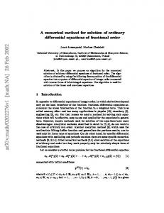
J. Math. & Stat., 8 (1): 77-81, 2012 blocks that contained the interpolation points involved in the derivation of the block method. According to Fig. 1, the method will generate the numerical solution at two points simultaneously. The values of yn+1 and yn+2 at the points xn+1 and xn+2 respectively are simultaneously computed in a block with step size h using the same back values which is the values at the point xn, xn-1 and xn-2 with step size rh. The formulae of 2-point block method are derived by integrating Eq. 1 d times as follows Eq. 2: Let xn+v = xn + vh, where v = 1 or 2. xn +v

x

xn

xn

∫ ∫

Fig. 1: 2-point block method Table 1: Coefficients when r = 1

x

… ∫ y d (x, y,…, y d −1 ) dxdx …dx = xn

xn +v

x

xn

xn

∫ ∫

(2)

x

… ∫ f (x, y,…, y d −1 ) dxdx …dx

r =1

β1,g −2

β1,g −1

g β1,0

g β1,1

g β1,2

g =1

11 720 11 1440 23 10080 61 120960 65 725760

−

74 720 76 − 1440 162 − 10080 436 − 120960 470 − 725760

456 720 582 1440 1482 10080 4638 120960 5700 725760

346 720 220 1440 370 10080 860 120960 838 725760

−

r =1

βg2, −2

βg2, −1

βg2,0

βg2,1

βg2,2

g =1

1 90 1 90 9 630 16 1890 80 22680

4 90 8 − 90 64 − 630 112 − 1890 560 − 22680

24 90 78 90 516 630 912 1890 4800 22680

124 90 104 90 384 630 464 1890 1840 22680

29 90 5 90

g=2

xn

g=3

which leads to the general formula below: y

d−g n+v

g −1

( vh )

k =0

k!

=∑

k

(d − g + k )

yn

+∫

xn+v

xn

( xn+v − x) ( g − 1)!

g

g=4

f ( x, y,..., y

d −1

) dx

(3)

g=5

where, g is the number of times which Eq. 3 is integrated over the corresponding interval. Lagrange interpolation polynomial is used to approximate the function of f ( x, y,..., yd −1 ) in Eq. 3 and the interpolation

g=2

points involved for the corrector formulae are

g=3

x − xn+2 and dx = hds ( x n − 2 ,f n − 2 ) ,..., ( x n + 2 ,f n + 2 ) . Let s = h

g=4

will be substitute into Eq. 3. By taking d = 5 in Eq. 1, the approximate solution of yn+1 and yn+2 will be obtained by integrating Eq. 1 once, twice, thrice, four times and five times over the interval [ x n , x n +1 ] and

g=5

evaluated using MAPLE and the corrector formulae in terms of r will be obtained. The same approaches were employed in the derivation of the predictor formulae for y, y′, y′′, y′′′, y( iv) at the points xn+1 and xn+2 respectively and the interpolation points involved are ( x n −3 ,f n − 3 ) ,..., ( x n ,f n ) .

αYm = hβYm′ + h 2λYm′′ + … + h d ξFm

( vh )

k=0

k!

y nd −+gv = ∑

y(n

d −g + k )

+

h

g

2

( g − 1)! j∑ =−2

βgv, jf n + j

(5)

where, α, β, λ and ξ are the coefficients of the 2-point block method. By applying the formulae for the constants Cq in Fatunla (1991), the order and error constant of the method will be obtained and the formulae are defined by Eq. 6:

Hence, it will produce the predictor formulae in terms of q and r. For the sake of simplification, the general corrector formula of 2-point block method is developed in the manner shown in Eq. 4: k

5 630 20 − 1890 112 − 22680 −

The order of this developed method is calculated in a block form as proposed by Fatunla (1991). The 2point block method for ODEs can be written in a matrix differentiation Eq. 5 below:

[ x n , x n + 2 ] respectively. Finally, this integral will be

g −1

−

19 720 17 − 1440 33 − 10080 83 − 120960 85 − 725760

(4)

∑α

C1 =

∑ ( jα

C2 =

βgv, j in Eq. 4 stands for the coefficients of the formulae

. . .

and tabulated in Table 1-3 for r = 1, r = 2 and r = 0.5. 78

k

C0 =

j= 0 k

j

j= 0 k

 j

j

− βj)

2

∑  2!α j= 0



j

 − jβ j − λ j  

J. Math. & Stat., 8 (1): 77-81, 2012 Cq =

k

 jq

∑  q ! α j= 0



j

−

 jq − 1 jt βj −… − ξ  ( q − 1 )! ( t − 1 )! j 

Table 4: Error constant for corrector formulae when r=1 D 1 2 3 4 5

(6)

Table 2: Coefficients when r = 2

Cp + d

r=2

β1,g −2

β1,g −1

g β1,0

g =1

37 14400 19 14400 81 201600 109 1209600 47 2903040

−

335 14400 175 − 14400 755 − 201600 1025 − 1209600 445 − 2903040

7455 7808 565 − 14400 14400 14400 4965 2656 265 − 14400 14400 14400 25995 9344 1065 − 201600 201600 201600 41475 11216 1375 − 1209600 1209600 1209600 20685 4480 575 − 2903040 2903040 2903040

r=2

βg2, −2

βg2, −1

βg2,0

βg2,1

βg2,2

g =1

−

1 900 1 450 8 3150 14 9450 14 22680

5 900 10 − 450 75 − 3150 130 − 9450 130 − 22680

285 900 345 450 2220 3150 3930 9450 4170 22680

1216 900 544 450 2112 3150 2656 9450 2176 22680

295 900 20 450 65 − 3150 170 − 9450 182 − 22680

g=2 g=3 g=4 g=5

g=2 g=3 g=4 g=5

g β1,1

g β1,2

β1,g −2

g =1

145 1800 70 1800 285 25200 185 75600 155 362880

g=2 g=3 g=4 g=5

β1,g −1

g β1,0

704 1635 1800 1800 352 975 − 1800 1800 1472 4740 − 25200 25200 976 3585 − 75600 75600 832 3435 − 362880 362880 −

g β1,1

g β1,2

755 1800 220 1800 695 25200 385 75600 289 362880

−

31 1800 13 − 1800 48 − 25200 29 − 75600 23 − 362880

r = 0.5

βg2, −2

βg2, −1

βg2,0

βg2,1

βg2,2

g =1

−

20 225 10 225 220 3150 400 9450 400 22680

64 225 64 − 225 1152 − 3150 2048 − 9450 2048 − 22680

15 225 240 225 3390 3150 6000 9450 6240 22680

320 225 250 225 1740 3150 2000 9450 1520 22680

71 225 14 225 2 3150 52 − 9450 64 − 22680

g=2 g=3 g=4 g=5

 37  10080    367  1  20160    315 

 419   302400     16     675 

 293   302400     188     4725 

The method is of order p if Cq = 0, q = 0(1) p + d1, Cp+d ≠ 0. Thus, by implementing this approach to the 2-point block method, we found that the predictor is of order four and corrector is of order five. The error constant for the corrector formulae when r = 1 will be in matrix form as shown in Table 4. Implementation of the method: A single code of the PECE scheme has been implemented with variable step size to study the computational time and human effort saving in using a direct integration method. The developed code starts by calculating the initial step size then finding the initial points in the starting block of the method. In order to evaluate the initial three starting points, the Euler method was adopted in the code as a generator of the method. Hence, the Euler method will be used only once at the beginning of the code. Once the points for starting block are calculated, then the block method can be applied until the end of interval. A test for checking the end of the interval is made in order to reach the end of the interval precisely and it will be functional at each step of integration. The strategy is by limiting the choices of the next step size to half, double or remains constant as the previous step size. At each step of the integration, if the approximated solutions fulfilled the desired accuracy, therefore the step is called as successive step. Hence, the choices for the next step size will be doubled or constant which specified by step size controller. Otherwise the step is called failure step and the next step size becomes half. The possible ratios for the next constant step size are (r = 1, q = 1), (r = 1, q = 2) and (r = 1, q = 0.5). At each doubled step size the ratios are (r = 0.5, q = 0.5) and (r = 0.5, q = 0.25). In the case of failure step size, the ratio is (r = 2, q = 2). A step failure happens due to the Local Truncation Error (LTE) exceeding the given tolerance. This corrector formulae show that, the code consist the formula of y, y′, y′′, y′′′ and y(iv). Hence, the developed algorithm could be use for solving first order up to fifth order problem of ODEs directly in a single code. The algorithm was written in C language. The approximation value of yn+1 and yn+2 are using predictor-corrector mode, (PkE) (Ck+1E)u where Pk and Ck+1 indicate the predictor of order k and corrector of order k+1 respectively and E indicate the evaluation of

Table 3: Coefficients when r=0.5

r = 0.5

 11  1440     1  −   90 

79

J. Math. & Stat., 8 (1): 77-81, 2012 the function. In the code, the corrector will be iterated until it is converge and the convergence test employed was Eq. 7: y (n +)2 − y(n + 2 ) < 0.1 × TOL u −1

u

2PRVS: Algorithm of 2-point fully implicit block method by reducing the problem to first order ODEs in Majid (2004) 2PDVS: Implementation of 2-point block method in this study by solving the problem directly

(7)

Problem 1: where, u is the number of iterations. The LTE will be obtained by comparing the absolute difference of the corrector formula derived of order k with the similar corrector formula of order k+1 at the point xn+2. If the LTE