numerical solution of some nonlocal, nonlinear dispersive ... - CiteSeerX

NUMERICAL SOLUTION OF SOME NONLOCAL, NONLINEAR DISPERSIVE WAVE EQUATIONS Beatrice Pelloni() and Vassilios A. Dougalis()

(*) Department of Mathematics Imperial College of Science, Technology and Medicine London SW7 2BZ, UK. (**)Department of Mathematics, University of Athens Panepistemiopolis, Zographou 15784, Greece. Submitted October 1997; in revised form February 1999 27 pages, 9 Figures, 3 Tables

Abstract

We use a spectral method to solve numerically two nonlocal, nonlinear, dispersive, integrable wave equations, the Benjamin-Ono and the Intermediate Long Wave equations. The proposed numerical method is able to capture well the dynamics of the solutions; we use it to investigate the behaviour of solitary wave solutions of the equations with special attention to those, among the properties usually connected with integrability, for which there is at present no analytic proof. Thus we study in particular the resolution property of arbitrary initial pro les into sequences of solitary waves for both equations and clean interaction of BenjaminOno solitary waves. We also verify numerically that the behaviour of the solution of the Intermediate Long Wave equation as the model parameter tends to the in nite depth limit, is the one predicted by the theory.

MSC numbers: 65M70, 35S10, 76B15 PAC numbers: 47.11+g, 47.20Ky, 83.10Ji

1

1 Introduction In this paper we shall consider two model equations that describe the one-way propagation of long waves in weakly nonlinear, dispersive media. The equations are of the form ut + ux + uux + Aux = 0; (1.1) where u is a real-valued function of (x; t) 2 (?1; 1)  [0; 1), and A is a linear operator whose action on ux models the dispersive eects. Perhaps, the best known example of an equation of the type (1.1) is the Korteweg-deVries (KdV) equation, that was originally derived a century ago as a model of surface water waves that propagate in one direction along a horizontal channel, and that have small amplitude and long wavelength relative to the depth of the water in the channel. The KdV equation is the PDE that corresponds to choosing A as the dierential operator Af(x) = fxx (x) in (1.1). Other choices include appropriate nonlocal (integrodierential) operators, whose symbol () (de ned by F Af() = ()F f(), F the Fourier transform) is no longer a polynomial in ; the form of () can be chosen to model particular dispersion relations. The speci c equations of the type (1.1) that we shall consider in this paper, namely the Benjamin-Ono (BO) and the Intermediate Long Wave (ILW) equations, have such nonlocal dispersive terms. The BO equation [8], [29], was derived by Benjamin as a model for internal waves in an incompressible strati ed uid with a density that varies only in a layer (pycnocline) whose thickness is much smaller than the total depth. (The wavelength of these waves is large with respect to the thickness of the layer.) We shall write it in the form ut + ux + uux + Huxx = 0;

(1.2)

where H is the Hilbert transform de ned by the principal value integral Z 1 f(y) dy: Hf(x) = ? 1 p:v: ?1 x ? y Existence and uniqueness of global solutions of the initial-value problem for the BO equation has been established by Iorio [17] and by Abdelouhab et al. [1]. In the latter reference, the continuous dependence of the solution on the initial data is also established. The ILW equation,[19], [22], is also a model for the propagation of long internal waves in an incompressible, strati ed uid, whose density varies again in a thin pycnocline located, for example, between a heavier and a lighter layer. The form of the ILW that we will use is that of [1]; it corresponds to an ILW derived by Kubota et al. [22], when the pycnocline is located at the bottom, below a layer of lighter uid whose thickness is proportional to a positive parameter 2

. In this form, the equation is

ut + (1 + 1 )ux + uux + Kuxx = 0;

(1.3)

where K is the integral operator Z 1 (x ? y) coth 2 f(y)dy: Kf(x) = ? 21 p:v: ?1 The global well-posedness of the initial-value problem for the ILW equation has been established in [1]; there, it is also shown that as  ! 1, its solutions converge, in an appropriate sense, to corresponding solutions of the BO equation. In addition, it is shown in [1] that suitably scaled solutions of the ILW converge as  ! 0 to solutions of the KdV equation; see also [34] for a discussion of the relevant physical modelling. These long wave model equations share with the KdV and other nonlinear dispersive wave equations the remarkable property that their nonlinear and dispersive terms are balanced in a manner that allows the existence of solitary wave solutions. Formulae for such solutions were found in [8] and [19] for the BO and the ILW, respectively. The de ning property of these solitary waves is that they are exceptionally stable: they travel at constant speed for long distances without undergoing any visible alterations in shape. This was already observed by Benjamin in his experiment with internal waves reported in [8]; we refer the reader to the bibliography of [6] for other references to existing experimental evidence. Orbital stability for these solitary waves has been rigorously established for the BO in [9] and [6], and for the ILW in [6] and [5]. It should also be noted that an added feature attesting to the stability of the solitary waves is that any initial waveform carrying sucient mass is eventually resolved into a number of solitary waves plus a trailing, oscillatory, dispersive tail. This property, that the BO and ILW share of course with other nonlinear dispersive wave equations, has also been observed in experiments and in computations , cf. e.g. [22], [26] and section 5 of the paper at hand. It is well known that when two solitary wave solutions of a class of equations including KdV interact with each other, they emerge from the interaction unchanged in shape and speed (modulo possible phase shifts). Moreover this interaction does not introduce any other alteration in the surrounding environment of the waves, for example in the form of a dispersive tail. When solitary wave solutions of a particular equation have this property of 'clean interaction', the underlying nonlinear equation is called integrable, and the solitary waves solitons. Thus, clean interaction observed e.g. beyond numerical doubt in a computational experiment may serve as an indication of possible integrability. Integrability is a very special and important property; cf. [4], [28] for general discussions of its manifestation and of solitons. An integrable equation admits an in nite number of conservation laws and it can be written as the compatibility 3

condition of two linear equations, called the Lax pair. This last property is the basis of the spectral analysis of these equations and for the de nition of inverse scattering transformations, [11]. The best known integrable PDE is of course KdV. It was indeed the rst equation for which spectral transform techniques yielded a complete analysis, started in [16], of all the features of integrability. Recently, a new approach to spectral analysis has widened the wealth of results for local integrable equations, [13], [14]. The BO and ILW equations are known to be integrable in some sense, cf. e.g. [2], [21], but the nonlocal character of their dispersive terms makes the analytical investigation of these equations much more dicult and the results so far obtained are not as satisfactory as in the case of integrable equations with local terms; for example, the integrability results derived in [2] are formal. Rigorous results concerning the inverse scattering transform method for BO require a certain small norm assumption that excludes solitary waves, [12]. Recently, some progress has been made [20], which seems to indicate that the small assumption can be dropped. At present, though, many properties of solitary wave solutions, among which clean interaction and asymptotic properties such as the number of solitons emerging from a given initial pro le, have not yet been established rigorously. The situation for the ILW equation is similar. For the above reasons, it is especially important to have a reliable and ef cient numerical method to study these nonlocal integrable equations and the behaviour of their solutions; although the properties of solitary wave solutions exhibited by local integrable models are expected to hold in these cases as well, there is at present no proof that they do. The preceding discussion of the equations under consideration and their solitary wave solutions properly applies to the initial-value problem, i.e. the problem of nding solutions of (1.2) or (1.3) for x 2 R and t > 0, given appropriate initial conditions u(x; 0) de ned on the real line. For the purposes of solving them numerically, we shall pose the equations on nite x-intervals [?L; L], and assume that the initial conditions, and, for each t > 0 the solutions u(:; t), are smooth periodic functions of period 2L. In the periodic case the dispersive operators H and K have dierent representations (cf. Section 2 and [1], [3]), which reduce to their de nitions on the real line as L ! 1. In addition, the real line formulae reduce to the periodic ones, when one applies H and K formally to periodic functions. We note that the associated initial- and periodic boundary-value problems have been proved in [1] to be globally well-posed. In this paper we shall approximate numerically, by a periodic code, solutions of the initial-value problem that decay to zero as jxj ! 1. Such solutions include the solitary waves of BO and ILW on the real line and the byproducts of their interactions. It is known that solitary waves decay quadratically in x for the BO, and exponentially for the ILW (cf. Section 4). Hence, by taking the interval [?L; L] large enough in each numerical experiment, so that the solution remains suciently small at the endpoints, we can approximate in a satisfactory 4

manner the generation and interaction of real line solitary waves for nite time intervals. Control of the boundary values is of course harder to maintain in the BO case of algebraic decay. The presence of the nonlocal terms in (1.2) and (1.3), which have a convenient Fourier representation in the periodic case (cf. Section 2), makes spectraltype methods the techniques of choice for approximatingtheir solutions. Spectral methods for nonlinear dispersive wave equations, with nonlocal terms dierent from the ones considered herein, were used in the computational study of Fornberg and Whitham, [15]. The split-step scheme advocated in [15] was used by Kubota et al. in [22] to integrate numerically in time the ILW equation in the case of two initial pro les, of short and long wavelength respectively. In [18], James and Weideman compared, in a computational study of the BO, a spectral method equipped with the usual Fourier basis in space, with one with a rational function basis on a nonuniform grid. The latter scheme is a natural candidate in view of the algebraic decay of the BO solitary waves, and it was argued in [18] that it has some advantages for small-time calculations. However, for longer time spans the Fourier method proved superior, provided the length of the spatial periodicity interval and the number of Fourier points were taken suciently large. The BO equation was also solved by a spectral method by Miloh et al., [26], wherein the authors veri ed computationally a formula giving the approximate number of solitary waves in which an initial pro le is resolved for t > 0. We are aware of three works containing rigorous convergence results for numerical methods for nonlinear, nonlocal ,dispersive wave equations.Pasciak, [30], analyzed semidiscrete spectral methods for a regularized analog of (1.1), wherein Aux is replaced by ?But , with B a pseudodierential operator generalizing e.g. d2=dx2. In a work more relevant to the equations considered in the paper at hand, Thomee and Vasudeva Murthy, [35], analyze a fully discrete nite dierence method for the initial- and periodic boundary-value problem for the BO. The method is unconditionally stable and is shown to be of second-order accuracy in space and time, in L2. It is based on a Crank-Nicholson time-stepping scheme , which is coupled with a "hybrid" spatial discretization , wherein the nonlinear term is approximated by conservative dierencing and the nonlocal, integral term by means of the midpoint quadrature formula which is interpreted as a discrete convolution and computed by discrete Fourier transforms .In [33] we proved L2 error estimates for the semidiscrete Fourier-Galerkin spectral method for the BO equation.(See also [32]). In the paper at hand we use a fully discrete spectral collocation method to study numerically the BO and ILW equations. The paper is organized as follows. In Section 2, we set the notation, describe the initial- and periodic boundaryvalue problem, and survey brie y the theory of existence and uniqueness of its solutions. In Section 3, we de ne two spectral discretization schemes in the spatial variable, namely the standard Fourier-Galerkin and a collocation method. 5

We use the latter scheme in our computations, coupling it with an explicit, fourth-order Runge-Kutta scheme for the discretization of the temporal variable. In Section 4 we present numerical results that validate the accuracy and stability of the fully discrete scheme; speci cally, we compute the temporal order of convergence to nd that it is the expected one, we compare the computed solutions with the exact form of the solitary waves in various error measures, and check the numerical conservation of some of the invariants of the equations. Finally, in Section 5 we present the results of our detailed numerical study. For the BO equation we investigate numerically resolution into and interaction of solitary waves. We rst consider the resolution of an arbitrary initial waveform of sucient mass into solitary waves; we show the results of several experiments, indicating that the number of resolved solitary waves con rms the predictions of [24], [26], [27]. Then we consider the interaction of BO solitary waves of dierent amplitude; the outcome of these experiments provides evidence of the fact that the interaction of two BO solitary waves leaves them unaltered, except for a phase shift. In our experiments we did not detect the appearance of a dispersive tail, consistently with the integrability of the BO equation. We have obtained similar soliton interaction results for the ILW equation, but we show here the BO case, which is harder to integrate as the solution decay in space quadratically. For the ILW equation we investigate numerically the resolution property: as in the BO case, we observe how an initial Gaussian waveform is resolved into one or more solitary waves plus a dispersive tail. Then we consider the asymptotic behaviour of solutions of the ILW equation as the parameter  becomes large; from the modelling point of view, one should recover the deep water model, the BO equation (see e.g. the discussion in [34]; this is analytically proven for the Cauchy problem posed on the real line, [1]). We integrate the BO and the ILW equations starting with the same initial pro le up to the same nal time, and we observe very good agreement of the nal pro les for  = 100 and agreement within graph thickness for  = 1000. A large part of the work presented is taken from the thesis of Pelloni [31]. A preliminary version of some of the BO computational results appeared in [33].

2 Notation and preliminary results We shall consider functions that are periodic of period 2. The function spaces we use are L2 and the Sobolev spaces Hr for integer r  0; these spaces will always be considered on [?; ] and their elements will be periodic functions. We denote by (
;
) the standard L2 inner product; this yields a norm in L2 which we denote by k
k. The norm in Hr , denoted k
kr , is de ned by

kf kr =

X kZ

(1 + k 6

2

^ j2 )r jf(k)

!=

1 2

:

(2.1)

^ k  Z, the Fourier coecients of f: As usual, we denote by f(k), Z ?ikx ^ = 1 f(k) 2 ? e f(x)dx: We recall that the Fourier coecients of the pointwise product fg are given by the convolution of the Fourier coecients of f and g, de ned by X ^ (f^  g^)(k) = f(m)^g (n): m;n  Z; m+n=k

We also need to consider discrete analogues of the quantities de ned above. To this end, for a positive integer N, consider the space SN de ned by SN = span fexp(ikx) : k  Z; ?N  k  N g :

(2.2)

Given the Fourier points xj = (j ?NN) ; j = 0; : : :; 2N;

and given f and g two continuous 2-periodic functions, we de ne the sesquilinear form 2N X (f; g)N = 2N2+ 1 f(xj )g(xj ): (2.3) The discrete Fourier coecients of f are

j =0

2N X f~k = 2N1+ 1 f(xj )e?ikx ; k = ?N; : : :; N; j

j =0

and it is then easy to verify that the trigonometric polynomial PI f(x) =

N X f~k eikx

(2.4)

k=?N

interpolates f at the points xj . The trigonometric polynomialPI f is the discrete inverse Fourier transform of f and can be computed eectively, given the values of f at the points xj , by the FFT algorithm. On SN , the sesquilinear form (2.3) is an inner product, and gives rise to the following L2 discrete norm

1= 0 N X kf kN = @ 2N2+ 1 jf(xj )j A : 1 2

2

2

j =0

7

We shall also consider the H1 discrete norm

1= 0 N X 2 kf k ;N = @ 2N + 1 (1 + j )jf(xj )j A : 1 2

2

2

1

2

j =0

It is known (cf. [10], [25]) that if f is in SN , then kf k = kf kN and kf k1 = kf k1;N . With this notation in place, we consider the initial- and 2-periodic boundaryvalue problem for the BO and ILW equations; thus we seek a real-valued function u(x; t), 2-periodic in x, that satis es  u + ()u + uu + Tu = 0; x  [?; ]; t  0; t x x xx (2.5) u(x; 0) = u0(x); x  [?; ]: Here () is a coecient equal to 1 for the BO and to 1+ 1 for the ILW case, and u0 is a real-valued. 2-periodic function on [?; ], describing the initial form of the wave. The nonlocal operator T is the appropriate form of the operators H and K (see Section 1) when they act on 2-periodic functions on [?; ]. For f in L2 , it is well-known that in the BO case (cf.e.g. [1]) the Fourier representation of Tf is the trigonometric sum X ^ ikx ; Tf(x) = i sgn(k)f(k)e (2.6) kZ

while for the ILW equation (cf. [3], [1]) Tf is given by X ^ ikx : coth(k)f(k)e Tf(x) = i k  Znf0g

(2.7)

From these expressions, it is easy to verify that in both cases T is antisymmetric in L2, and that it commutes with dierentiation. The well-posedness of the initial-value problem (2.5), with T given by (2.6) or (2.7), was analyzed in Section 9 of [1]. For example, in Theorem 9.1 of [1] it is proved among other that if u0 2 Hr , where r  2, then there is a unique solution u of (2.5) continuous and bounded on [0; 1) with values in Hr . We nally note that, being integrable, both the BO and the ILW equations have in nitely many invariants; the rst three are R  u(x; t)dx: Integral mean: ?

L norm: 2

R  u (x; t)dx: ? 2

R

Third invariant: ? [uxT(u) ? 31 u3]dx: The invariance of these expressions is easily shown for smooth solutions by using periodicity and the properties of T. More on the BO and ILW invariants can be found in [1]. 8

3 The discrete scheme

Space semidiscretizations

We shall now approximate the solutions of (2.5) in space by elements of the nite-dimensional space SN de ned in (2.2), leaving for the time being the temporal variable continuous. We shall consider two such semidiscretizations of (2.5). The semidiscrete Fourier-Galerkin (spectral) approximation to (2.5) is a map U from [0; 1) to the real-valued elements of SN such that, for all 'SN :

 (U + ()U + UU + TU ; ') = 0; t  0; t x x xx U(
; 0) = PN u0;

(3.1)

where PN denotes the orthogonal projection of L2 onto SN . By choosing ' = eikx for k = ?N; : : :; N, we see that (3.1) is an initial^ t) of U(x; t), value problem for an ODE system for the Fourier coecients U(k; which, by standard ODE theory, has a unique solution at least locally in time. The existence of a solution for all t  0 is a consequence of the fact that (3.1) is conservative in L2. In fact, this semidiscretization preserves the rst three invariants of (2.5). The proof of this fact follows exactly its continuous counterpart. In [33] (and in full detail in [32]) we analyze the convergence of this scheme using the techniques of [7]. We prove that if u0 belongs to Hr for some r  2, then, for each 0  t < 1 there holds that (3.2) max ku ? U k  NCr?1 : 0tt This rate of convergence in the L2 norm matches the rate proved e.g. in [23] for spectral (Galerkin) approximations of the KdV equation with initial data in Hr . The Fourier-Galerkin scheme just described has the attractive property of possessing at least some of the conservation laws of the equation. Nevertheless, to be able to use such a scheme in practice, one needs to compute the Fourier coecients of the initial value u0 exactly; more importantly, the computation of the nonlinear term as a convolution product is expensive. Thus, in actual computations, one usually resorts to a collocation scheme (see e.g. [10], [25]). Given SN as before, we de ne the collocation semidiscrete approximation to the solution of (2.5) as the map U from [0; T] to the real-valued elements of SN such that for all j = 0; : : :; 2N  (U + ()U + UU + TU ) (x ) = 0; t  0; t x x xx j (3.3) U(xj ; 0) = u0 (xj ): 9

Recall that (
;
)N denotes the discrete inner product on SN de ned by (2.3); PI is the interpolation operator at the Fourier points xj de ned by (2.4), and @N is the composition @xPI . (Note that if ' 2 SN , (PI v; ')N = (v; ')N for all continuous v, and 'x = @N '.) Then the ODE system (3.3) can be equivalently formulated as the problem of nding the map U as above, which, for all ' in SN , satis es  (U + ()U + UU + TU ; ') = 0 t  0; t x x xx N (3.4) U(0) = PI u0 : To see this, for k = ?N; : : :; N, choose ' = eikx in (3.4). Then for the ~ (supdiscrete Fourier coecients of U we have by de nition (U; ')N = 2U(k) pressing the t-dependence). Similarly, the discrete Fourier coecients of @N U ~ are given by ikU(k): De ne (k) = isgn(k) for the BO case, and (k) = icoth(k); k 6= 0, (0) = 0 for the ILW case; then the discrete Fourier coef~ A discrete inverse transform then yields the cients of T@N2 U are ?k2 (k)U(k): values Ux (xj ) and TUxx (xj ), j = 0; : : :; 2N, which appear in the system (3.3). The same standard ODE arguments used for the Fourier-Galerkin approximation yield the existence of a solution of (3.3) locally in time. This scheme does not preserve the invariants of the equation, except the mean; one could modify the nonlinear term by writing it as uux = (1=3)uux + (1=3)(u2)x , and then approximating it by (1=3)PI (UUx ) + (1=3)@N (U 2). The scheme obtained in this way preserves the L2 norm (which would allow one to extend the existence argument to all t  0), but it fails to preserve either the rst or third invariants; moreover it implies one extra nonlinear computation. Although we do not have at present a convergence estimate for the collocation scheme (3.3), our numerical experiments (cf. section 4) suggest that it approximates the solution of (2.5) well and that it preserves the rst three invariants to a high degree of accuracy. Thus we use (3.3), rather then the Fourier-Galerkin or the modi ed collocation scheme, as it is computationally faster and gives accurate results.

Time discretization

To discretize the system of ODE's (3.3) in the temporal variable, we used the classical, explicit, four-stage, fourth-order Runge-Kutta method, which in the case of the ODE initial-value problem y0 = f(y; t); t  0; y(0) = y0 ;

10

yields approximations yn to y(tn ), where tn = n
t, n = 0; 1; : : :, given by the formulas 4 X n;j n;j yn+1 = yn +
t 6 j =1 f(t ; y ); yn;1 = yn ; tn;1 = tn; n;1 n;1 n;2 n
t yn;2 = yn +
t (3.5) 2 f(t ; y ); t = t + 2 ; n;2 n;2 n;3 n
t yn;3 = yn +
t 2 f(t ; y ); t = t + 2 ; n;3 n;3 n;4 n yn;4 = yn +
t 2 f(t ; y ); t = t +
t:

When we apply this scheme to the ODE system represented by (3.3) we obtain approximations U m 2 SN of U(tm ) for m = 0; 1; 2; : : :. Since this ODE system (as well as its Galerkin counterpart (3.1)) is sti, we cannot expect explicit time-stepping methods like (3.5) to be stable unless we impose mesh conditions involving N and
t. The region of absolute stability of the Runge-Kutta method (3.5) includes an interval of the imaginary axis which is symmetric about the origin; thus it follows from the form of the system (3.3) that a constraint of the type
tN 2  C , for some constant C, will be sucient to guarantee stability of at least the linearized analog of (3.3). We observed in our numerical experiments that such a condition is sucient in the case of the nonlinear ODE system as well. We also note that the stability constraint that
tN 2 be small is not a serious drawback here, because spectral methods do not require large N to achieve good accuracy in approximating smooth solutions of problems in one spatial dimension, such as the ones under consideration.

4 Validation of the fully discrete scheme We validated the method described in the previous section in three dierent ways, namely by checking the temporal convergence rate, by verifying that the L2 norm and a discrete version of the third invariant of the numerical solution remain very close to constant as t grows, and by monitoring various types of error. We did this for both the BO and ILW equation, but record here only the BO results. We start with the temporal convergence rate. For the Runge-Kutta method used we expect this rate to be equal to four. To be able to compute the rate accurately, we solved numerically nonhomogeneous problems of the form ut + ux + uux + Huxx = f(x; t); (4.1) where the nonhomogeneous term f is determined by imposing that some known simple periodic function is an exact solution of (4.1). In such a computation, one 11

needs to ensure that the spatial error is small and does not pollute the temporal error. We recall that the spatial rate of convergence for spectral methods is exponential in the case of smooth solutions; this has been proved, cf. (3.2), for the Fourier-Galerkin method, and it is reasonable to expect that the same holds for the collocation scheme (3.3). In the particular test we report, we impose that u = A sin(x ? t) is an exact solution; then, since H(sin x) = ? cos x, we have f(x; t) = A cos(x ? t) sin(x ? t). Given two numerical solutions for the problem corresponding to the same N and dierent time steps
t1 and
t2 with errors 1 and 2 evaluated at the same value of t, the temporal rate of accuracy may be computed as 1 ; log 1 = log
t
t 2 2 provided that the spatial error is negligible. Table 1 shows the experimental temporal rate of accuracy as measured by the (normalized) L2 error of the fully discrete approximation U = U m at time t = tm , de ned by k; E0(t) = kU k?u u(t) 0k for a run with A = 0:1 on a spatial interval [?; ] at t = tm = 20. We took N = 128; for these parameters we estimated (by taking
t very small) the spatial error to be about 8:0E ? 10. Hence we have con dence in the computed temporal rates of Table 1, which show that the theoretical rate of four emerges clearly. Since our main goal in the paper at hand is to study numerically the generation and interaction of solitary wave solutions of the Cauchy problem for the BO and the ILW equations, we compared such exact solutions with the approximations generated by our numerical scheme evolving from initial data of the form BO : u0 (x) = us (x; 0) = c2 x4c ; 2+1 c?
: ILW : u0 (x) = us (x; 0) = cosh 2c x These initial values give rise to solitary wave solutions on the real line for t  0, [8], [19], given by the formulas (4.2) BO : us(x; t) = c2 (x ?4cct)2 + 1 ; ? c
ILW : us(x; t) = (4.3) cosh c (x ? (1 + c )t) ) : 2



Here c is a positive velocity parameter; in the ILW equation, we made the particular choice  = =c for the parameter . The decay of the tails of the BO 12


t E0(t) rate 0.0571 1.35875E-3 4.07 0.0380 2.60613E-3 3.79 0.0327 1.45799E-3 3.99 0.0286 8.42387E-3 Spatial error  8:0E ? 10 Table 1: Normalized L2 errors and temporal convergence rates at t = 20 (BO) solitary wave is then algebraic, as jxj ! 1, whereas for the ILW solitary wave, the decay is exponential The functions us solve the initial-value problem on the real line and are not periodic. For the BO, us(x; t) is a rational function which does not decay to zero very rapidly for each t. We use it as an \exact" solution for our periodic problem, noting that us(x; 0) is even, so that its values at the endpoints of any interval [?L; L] are equal. By choosing this interval large, these values can be made small enough for us (x; 0) to be considered as periodic function for computational purposes. In addition, taking L large enough ensures that for the time scales of our numerical experiments, the periodic problem approximates the problem on the real line well; for a discussion relevant to this point see also [18]. Of course, the ILW solitary wave solutions decay to zero very rapidly and thus can be considered periodic, provided that the interval [?L; L] is large enough. Therefore the BO is computationally more dicult; for this reason we report here only BO error calculations. To treat problems on [?L; L] in the code, we rescale the problem by a parameter " = L ; this amounts to solving numerically over [?; ] the equation ut + " (()ux + uux ) + "2 Tuxx = 0; with appropriately transformed initial conditions. To test the conservation properties of the scheme we performed several numerical experiments using as exact solutions the solitary wave pro les us given by (4.2). Some typical output is shown in Table 2; it corresponds to a run approximating the solitary wave for BO with c = 0:2 on the interval [?L; L] = [?150; 150] up to t = 50, with N = 512 and
t = 0:5. The rst two entries of Table 2 are the L2 norms of the approximate solution at t = 0 and t = 50 respectively. The next two are the absolute values, at these two instances of time, of a discrete version of the third invariant. Since the (negative of the) third invariant can be written as (u2 ; u) + (u; Hux), it is 13

kU(0)k kU(50)k jI(0)j jI(50)j

2.24197903 2.24197903 .0104904531 .0104904787 L21 error E0(50) 1.95272377E-4 H error E1(50) 1.95273090E-4 amplitude error 1.84473864E-6 phase error 2.25048192E-5 Table 2: Invariants and various errors. BO solitary wave, c = 0:2, t = 50. natural to de ne its discrete analogue as the sum of the two inner products (U 2; U)N + (U; HUx )N , and compute its value by the expression  2N  X 2 1 3 U (xj ) + U(xj )HU(xj ) : I(t) = 2N + 1 j =0 3

It is evident that both these quantities are conserved accurately by the fully discrete scheme. The last four entries of Table 2 are the values at t = 50 of various measures of error for this run. In addition to the normalized L2 error E0(t) de ned previously, we compute three other quantities of interest, namely:  The normalized H1 error k1 E1(t) = kU k?u u(t) 0 k1  The amplitude error, de ned as j ? maxx jU(t)j j: Eamp (t) = j maxx ju(t) maxx ju(t)j To compute a good approximation of the amplitude of the approximate solution U, for which we have values only at a discrete set of points, we pass a fourth-order interpolating polynomial through ve points near the peak of U and then take the maximum value of this polynomial as the actual maximum of the wave; the value of x at which this maximum is achieved is denoted by xmax . With this in hand, we can also compute  The phase error, de ned as Eph (t) = jxp ? xmax j; where xp is the point at which the exact solitary wave solution has its peak at time t. 14

1

exact computed

0.8 0.6 0.4 0.2 0

-50

0

50

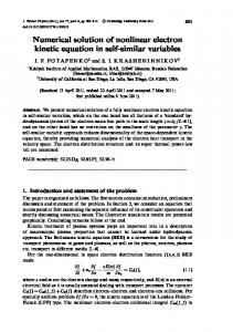
Figure 1: Exact vs. approximate solution. BO solitary wave, c = 0:2, t = 50. All these errors are quite small. Figure 1 shows the superimposed graphs of the numerical and exact solutions for this run at t = 50.

5 Numerical study of solitary waves In this section, we report on the outcome of various numerical experiments we performed using the scheme previously described and tested.

Results for the BO equation

It is well-known that solitary waves for the BO equation are orbitally stable, [9], [6]. To our knowledge, this important property is one of the very few special properties of solitary wave solutions that have been proved rigorously in the case of the BO equation. Here we study numerically the behaviour of these solutions, with the aim of establishing computational evidence for two other properties. The rst one is the resolution property: an arbitrary initial pro le of large enough size is resolved into one or more pulses, which are exact solitary wave solutions of the BO equation, plus a dispersive tail. This property shows that solitary waves play a very special and important role among all solutions of model equations for long waves, and it has been proved analytically for other 15

integrable equations. We checked the resolution property numerically by choosing as initial pro le the Gaussian u0 (x) = exp(?x2=144): We let the code run up to t = 200 on [?150; 150], with N = 512 and
t = :025. By that time (see Figure 2) the Gaussian pro le had resolved itself into two clearly de ned separate pulses travelling to the right, plus a dispersive oscillating tail. We computed the elevation of the rightmost peak of the numerical solution and superimposed on the graph a BO solitary wave of the same amplitude. Figure 2 shows that the two waves are identical to graph thickness. In Figure 3 we show the outcome of a similar comparison by superposition for the second, smaller pulse; again the graph shows clearly that the smaller pulse is to a good approximation a BO solitary wave. The resolution question has been previously addressed in [24], [26] and [27]. In these papers, the authors derive a formula which gives approximately the number of BO solitary waves that will be formed from a given initial waveform u0. (In [26], this formula is also veri ed by a numerical solution of the BO equation). In the particular case of a Gaussian of the form u0(x) = A exp(?(x=)2 ), the approximate number of solitary waves Nsol expected to eventually appear is given by (5.1) Nsol = A 4p  : In our case, A = 1 and  = 12, giving an approximate value of 1:7, which should be rounded to 2, and agrees with our experimental nding. We veri ed the validity of this formula further by running two more experiments, shown in Figure 4. In the rst one, the initial pro le is a Gaussian of amplitude A = 1 and width  = 9, which yields Nsol  1:3; the parameters of the run are N = 512,
t = 0:025, L = 150. At time t = 250, one solitary wave is clearly visible, followed by a tail that is dispersing behind. The largest oscillation behind the main peak is indeed decaying, as we veri ed by checking the solution at previous times: its height was equal to 0:2550, 0:2345 and 0:2200 at times t = 150, t = 200, and t = 250, respectively. In the second one, the initial pro le is a Gaussian of amplitude A = 1 and width  = 20, which yields Nsol  2:8; the parameters of the run are N = 1024,
t = 0:025, L = 200. At time t = 300, three solitary waves have been resolved, followed by a dispersive tail. The second property we investigate is the soliton property. We say that an equation has this property when two solitary waves, which are exact solutions of the equation, have a `clean' interaction, in the sense that they are not altered after interacting (modulo phase shifts), and do not leave dispersive oscillations in their wake. It is well-known that this is true for several local integrable models admitting solitary wave solutions, e.g. the KdV equation. Since BO is also integrable, we expect this property to hold; and this is indeed what is indicated by our numerical experiments. We studied the dynamics of this 16

2 1.8 1.6 1.4 1.2 1 0.8 0.6 0.4 0.2 0 -0.2 -150

numerical solution BO sol. wave

-100

-50

0

50

100

150

Figure 2: BO - Resolution of the Gaussian u0(x) = e?x2 =144, t = 200. Exact solution superimposed on the larger resolved pulse. 2 numerical solution 1.8 BO sol. wave 1.6 1.4 1.2 1 0.8 0.6 0.4 0.2 0 -0.2 -150 -100 -50 0 50 100 150 Figure 3: BO - Resolution of the Gaussian u0(x) = e?x2 =144, t = 200. Exact solution superimposed on the smaller resolved pulse. 17

2

resolved wave - Nsol = 1:3

1.5 1 0.5 0 -150

-100

-50

0

2.5

50

100

150

resolved wave - Nsol = 2:8

2 1.5 1 0.5 0 -0.5 -100

-50

0

50

100

150

200

Figure 4: BO - Resolution of the2 Gaussian u0 (x) = e?x2 =81 at t = 250 (above) and of the Gaussian u0 (x) = e?x =400 at t = 300 (below) . 18

Interaction 1 for t=0: peaks at ?100, 0, of amplitude A1 = 4, A2 = 1, resp. time amplitude 1 amplitude 2 phase shift 1 phase shift 2 160 3.8503 1.0202 0.496 -0.496 180 3.9479 1.0057 0.369 -0.370 200 3.9733 1.0019 0.325 -0.331 220 3.9869 1.0001 0.300 -0.301 240 3.9937 1.0001 0.296 -0.300 Interaction 2 for t=0: peaks at ?200, ?50, of amplitude A1 = 3, A2 = :4, resp. time amplitude 1 amplitude 2 phase shift 1 phase shift 2 300 2.9373 0.4052 0.431 -0.428 350 2.9829 0.4042 0.420 -0.422 400 2.9904 0.4028 0.450 -0.448 450 2.9979 0.4003 0.498 -0.487 500 2.9992 0.4001 0.500 -0.500 Table 3: Amplitude and phase shift for interacting pairs of BO solitary waves phenomenon, and followed the changes in amplitude and phase after interaction had occurred for a few pairs of interacting solitary waves of dierent amplitude. Pursuing further the analogy with the KdV case, we expect that the amplitudes of the two waves will be altered during the interaction, but will subsequently return to their original values. The only permanent change, after interaction has occurred, is expected to be a xed phase shift, to the right for the larger solitary wave, and to the left for the smaller one. We report in Table 3 data of two dierent experiments with interacting pairs of solitary waves; in both cases N = 1024 and
t = 0:02. The length 2L of the spatial interval was equal to 300 for the rst and 500 for the second case. In both examples, the wave of larger amplitude starts behind the smaller wave; after some time has elapsed, interaction occurs, and then the two waves emerge with the small behind the large one. In Table 3, we list the initial location of the two waves , and in Figure 5 we show the evolution of one of these pairs of solitary waves (with initial amplitudes A1 = 4 and A2 = 1), at four instances around the time of interaction. The data of Table 3 indicate clearly that after interaction has occurred, the only permanent change is a shift in the phase of the two solitary waves. As expected, the large wave in both cases has been shifted forwards by an amount indicated in the column "phase shift 1", and the small one backwards, by an amount indicated in the column "phase shift 2". The amplitude of the two waves 19

4 3.5 3 2.5 2 1.5 1 0.5 0 -0.5 -150

t=100

t=140

t=180

t=130

-100

-50

0

50

100

150

Figure 5: BO - Solitary wave interaction. A1 = 4, A2 = 1. changes around the time of interaction; the smaller wave is found to be slightly taller soon after interaction has occurred, while the large wave is a bit shorter. Nevertheless, if we let the solution evolve for longer times, the amplitudes slowly but steadily seem to return to the original values. A few comments on the accuracy of this numerical experiment are in order. Recall that the amplitude and phase of the numerical solution are computed with the aid of an interpolating polynomial of degree four near the apparent maximum; nevertheless, if the true numerical maximum occurs between the Fourier nodes at which the discrete solution is computed, a small error may be introduced. In addition, as we have remarked earlier, near the endpoints of the interval there is an error introduced by the periodic approximation of a non-periodic waveform; this error also aects the amplitude computed for large times, when the faster wave is near the right end of the interval, or has been wrapped around to re-enter at the left. For this reason the computation is performed only up to a time when the large solitary wave is still suciently far from the right endpoint. Modulo these remarks, the qualitative outcome of the experiment is quite clear and matches precisely the expected behaviour of solutions of integrable equations. The related, next series of experiments suggest that after the interaction, 20

4.5

t=380 t=0

4 3.5 3 2.5 2 1.5 1 0.5 0

-200

-100

0

100

200

Figure 6: BO - Solitary wave interaction: absence of dispersive tail 0.1 0.08 0.06 0.04 0.02 0 -0.02 -0.04

t=380

-200

-100

0

100

200

Figure 7: BO - Solitary wave interaction: absence of dispersive tail - Enlargement of part of Figure 6 at t=380

21

1.4

computed solution ILW sol.wave

1.2 1 0.8 0.6 0.4 0.2 0 -150

-100

-50

0

50

100

150

Figure 8: ILW - Resolution of the Gaussian u0(x) = e?x2 =25, t=100 when the two solitary waves have reappeared essentially unaltered in shape, no other disturbance is generated. The outcome of this experiment is shown in Figures 6 and 7. The initial pro le, dotted in Figure 6, is again a couple of BO solitary waves of amplitudes A = 4 and A = :8, whose centers are located at x = ?156:25 and x = 0 respectively. The full line shows the solution at t = 380, i.e. at a time after the large wave has overtaken the small one; in Figure 7 we show part of the same picture in a larger scale. It is evident that there is no hint of any oscillation behind the solitary waves after they have interacted. The run was made on the interval [?250; 250], with small steps, namely N = 2048 and
t = 0:001. The L2 norm of the wave is well preserved by the numerical scheme; in fact, we nd that jku0k ? kU(t)kj  10?8 at t = 380. We conclude that this experiment provides clear numerical evidence of the fact that, as in the case of the KdV, the interaction of two BO solitary waves does not produce any alteration in the surrounding environment in the form of a dispersive tail.

Results for the ILW equation

In the case of the ILW equation we focus our attention on two issues: the resolution property and the limit of the solutions as  ! 1. We rst report a computation of the evolution of a Gaussian initial pro le, as evidence for the resolution property. (Note that the ILW solitary waves are 22

known to be stable for all positive values of , [6], [5]). We took the Gaussian u0(x) = exp(?x2 =25) as the initial pro le on [?150 : 150], and integrated the ILW equation with  = =c with our code, using N = 512 and
t = 0:05, up to a time t = 100. By that time, a single solitary pulse had clearly formed and separated from the oscillatory part of the solution. We then compared the leading wave with the exact solitary wave solution of ILW of the form (4.3) having the same amplitude. The resulting graphs are plotted in Figure 8. It is evident, that what is produced is a solitary wave, to graph thickness, and that it is followed by an oscillatory part. We let this solitary wave travel for larger values of t and we observed no change in its shape or speed, of course before its interaction with the trailing tail took place. The second issue we address is the limit of solutions of the ILW equation as the depth parameter  becomes large. We expect these solutions to approach solutions of the deep water model, i.e. of the BO equation. A rigorous proof of this fact, for the Cauchy problem for the BO equation on the real line, is presented in [1]. The result proved in Theorem 8.1.1 of [1] is that for u0 in Hr , r  2, the solution of the ILW equation with parameter  approaches the solution of the BO equation corresponding to the same initial data, as  ! 1. (The limit is in Hr uniformly on bounded time intervals.) In Figure 9 we show the evolution of an initial BO solitary wave of unit amplitude computed by integrating numerically the BO and the ILW equations in two cases corresponding to  = 100 and  = 1000 in the ILW. The parameters of the run were N = 256,
t = :01 and the execution is stopped at t = 400. The agreement of the two solutions is visibly better when  = 1000.

Acknowledgements This work has been partially supported by the Institute of Applied and Computational Mathematics of the Foundation for Research and Technology - Hellas. The authors also wish to express their thanks to Prof. J. L. Bona for many discussions and suggestions relevant to the material of the paper.

23

1

BO solution ILW solution initial wave  = 100

0.8 0.6 0.4 0.2 0 -150 1

-100

-50

0

50

100

150

BO solution ILW solution initial wave  = 1000 100

0.8 0.6 0.4 0.2 0 -150

-100

-50

0

50

Figure 9: Behaviour of ILW as  ! 1, t=400

24

100

150

References [1] L. Abdelouhab, J.L. Bona, M. Felland, and J.-C. Saut. Nonlocal models for nonlinear, dispersive waves. Physica D, 40:360{392, 1989. [2] M.J. Ablowitz and A.S. Fokas. The inverse scattering transform for the Benjamin-Ono equation - a pivot for multidimensional problems. Studies in Applied Math., 68:1{10, 1983. [3] M.J. Ablowitz, A.S. Fokas, J. Satsuma, and H. Segur. On the periodic intermediate long wave equation. J. Phys. A: Math. Gen., 15:781{786, 1982. [4] M.J. Ablowitz and H. Segur. Solitons and the inverse scattering transform. SIAM, 1981. [5] J. P. Albert and J.L. Bona. Total positivity and the stability of internal waves in strati ed uids of nite depth. IMA J. of Applied Math., 46:1{19, 1991. [6] J. P. Albert, J.L. Bona, and D.B. Henry. Sucient conditions for stability of solitary-wave solutions of model equations for long waves. Physica D, 24:343{366, 1987. [7] G.A Baker, V.A. Dougalis, and O.A. Karakashian. Convergence of Galerkin approximations for the Korteweg-deVries equation. Math. Comp., 40:419{ 433, 1983. [8] T.B. Benjamin. Internal waves of permanent form in uids of great depth. J. Fluid. Mech., 29:559{592, 1967. [9] D.P. Bennett, R.W. Brown, S.E. Stans eld, J.D. Stroughair, and J.L. Bona. The stability of internal solitary waves. Math. Proc. Camb. Phil. Soc., 94:351{379, 1983. [10] C. Canuto, M.Y. Hussaini, A. Quarteroni, and T.A. Zang. Spectral Methods in Fluid Dynamics. Springer, New York, 1987. [11] R. Coifman and A.S. Fokas. The inverse spectral method in the plane. In A.S. Fokas and V.E. Zakharov, editors, Important developments in soliton theory, pages 58{85. Springer-Verlag, Berlin, 1993. [12] R. Coifman and V. Wickerhauser. The scattering transform for the Benjamin-Ono equation. Inverse Problems, 6:825{861, 1990. [13] A.S. Fokas. A uni ed transform method for solving linear and certain nonlinear pde's. Proc. Royal Soc. Series A, 453:1411{1443, 1997. 25

[14] A.S. Fokas and B. Pelloni. The solution of certain initial boundary-value problems for the linearized Korteweg-deVries equation. Proc. Royal Soc. Series A, 454:645{657, 1998. [15] B. Fornberg and G.B. Whitham. A numerical and theoretical study of certain nonlinear wave phenomena. Phil. Trans. Roy. Soc. London A, 289:373{ 404, 1978. [16] G.S. Gardner, J.M. Greene, M.D. Kruskal, and R.M. Miura. A method for solving the Korteweg-deVries equation. Phys. Review Lett., 19:1095, 1967. [17] R. Iorio. On the Cauchy problem for the Benjamin-Ono equation. Comm. P.D.E., 11:1031{1081, 1986. [18] R.L. James and J.A.C. Weideman. Pseudospectral methods for the Benjamin-Ono equation. In R. Vichnevetsky, D. Knight, and G. Richter, editors, Advances in Computer Methods for partial dierential equations VII, pages 371{377. IMACS, 1992. [19] R.I. Joseph. Solitary waves in a nite depth uid. J. Phys. A, 10:L225, 1977. [20] D.J. Kaup and Y. Matsuno. On the inverse scattering transform for the Benjamin-Ono equation. Stud. Appl. Math., 101:73{98, 1998. [21] Y. Kodama, J. Satsuma, and M.J. Ablowitz. Direct and inverse scattering problems of the nonlinear intermediate long wave equation. J. Math. Phys., 23:564{576, 1982. [22] K. Kubota, D.R.S. Ko, and L.D. Doobs. Weakly nonlinear, long internal gravity waves in strati ed uids of nite depth. J. Hydronautics., 12:157{ 165, 1978. [23] Y. Maday and A. Quarteroni. Error analysis for spectral approximation of the Korteweg- de Vries equation. M2AN Model. Math. et An. Num., 22(3):499{529, 1988. [24] Y. Matsuno. Asymptotic properties of the Benjamin-Ono equation. J. Phys. Soc. Japan, 51:667{674, 1982. [25] B. Mercier. An introduction to the numerical analysis of spectral methods. Lectures notes in Physics No. 318. Springer, New York, 1983. [26] T. Miloh, M. Prestin, L. Shtilman, and M.P. Tulin. A note on the numerical and N-soliton solutions of the Benjamin-Ono evolution equation. Wave Motion, 17:1{10, 1993. [27] A.A. Minzoni and T. Miloh. On the number of solitons for the intermediate long wave equation. Wave Motion, 20:131{142, 1994. 26

[28] A. Newell. Solitons in Mathematics and Physiscs. CBMS-NSF, Philadelphia, 1985. [29] H. Ono. Algebraic solitary waves in strati ed uids. J. Phys. Soc. Japan, 39:1082{1091, 1975. [30] P.E. Pasciak. Spectral methods for a nonlinear initial value problem involving pseudo dierential operators. SIAM J.Numer.Anal., 19:142{154, 1982. [31] B. Pelloni. Spectral methods for the numerical solution of nonlinear dispersive wave equations. PhD thesis, Yale University, 1996. [32] B. Pelloni and V.A. Dougalis. Spectral numerical schemes for a class of nonlinear nonlocal equations. To appear. [33] B. Pelloni and V.A. Dougalis. On spectral methods for the Benjamin-Ono equation. In E.A. Lipitakis, editor, HERMIS '96, Proceedings of the third Hellenic-European conference on Mathematics and Informatics, pages 229{ 237, LEA, Athens, 1996. [34] M.G. Rose. Weakly nonlinear long waves models in strati ed uids. PhD thesis, Pennsylvania State University, 1991. [35] V. Thomee and A.S. Vasudeva Murthy. A numerical method for the Benjamin-Ono equation. BIT, 38:597{611, 1998.

27