IEEE/CAA JOURNAL OF AUTOMATICA SINICA
1
Numerical Solution of the Distributed-Order Fractional Bagley-Torvik Equation Hossein Aminikhah, Amir Hosein Refahi Sheikhani, Tahereh Houlari and Hadi Rezazadeh
Abstract—In this paper, two numerical methods are proposed for solving distributed-order fractional Bagley-Torvik equation. This equation is used in modeling the motion of a rigid plate immersed in a Newtonian fluid with respect to the nonnegative density function. Using the composite Boole’s rule the distributedorder Bagley-Torvik equation is approximated by a multi-term time-fractional equation, which is then solved by the GrunwaldLetnikov method (GLM) and the fractional differential transform method (FDTM). Finally, we compared our results with the exact results of some cases and show the excellent agreement between the approximate result and the exact solution. Index Terms—Bagley-Torvik equation, distributed-order, fractional, fractional differential transform method, GrunwaldLetnikov method.
I. I NTRODUCTION
T
HE fractional order calculus establishes the branch of mathematics dealing with differentiation and integration under an arbitrary order of the operation, that is the order can be any real or even complex number, not only the integer one. Although the history of fractional calculus is more than three centuries old, it only has received much attention and interest in the past 20 years; the reader may refer to [1], [2] for the theory and applications of fractional calculus. The generalization of dynamical equations using fractional derivatives proved to be useful and more accurate in mathematical modeling related to many interdisciplinary areas. Applications of fractional order differential equations include: electrochemistry [3], porous media [4] etc. The fractional differential operator of distributed order Z γ2 w(α) Dt f (t) = w(α)Dtα f (t)dα, w(α) ≥ 0 (1) γ1
This article has been accepted for publication in a future issue of this journal, but has not been fully edited. Content may change prior to final publication. Recommended by Associate Editor Dianwei Qian. (Corresponding author: Hossein Aminikhah.) Citation: H. Aminikhah, A. H. R. Sheikhani, T. Houlari and H. Rezazadeh, “Numerical solution of the distributed-order fractional bagley-torvik equation,” IEEE/CAA Journal of Automatica Sinica, pp. 1−6, 2017. DOI: 10.1109/JAS.2017.7510646. H. Aminikhah and T. Houlari are with the Department of Applied Mathematics, Faculty of Mathematical Sciences, University of Guilan, Rasht 41938-19141, Iran (e-mail:
[email protected]; tahereh−
[email protected]). A. H. R. Sheikhani is with the Department of Applied Mathematics, Faculty of Mathematical Sciences, Islamic Azad University, Lahijan Branch, Lahijan 1616, Iran (e-mail: ah−
[email protected]). H. Rezazadeh is with the Faculty of Engineering Technology, Amol University of Special Modern Technologies, Amol 46168-49767, Iran. He is also with the Department of Applied Mathematics, University of Guilan, Rasht 41938-19141, Iran(e-mail:
[email protected]). Color versions of one or more of the figures in this paper are available online at http://ieeexplore.ieee.org.
α
d is a generalization of the single order Dα = dt α (α ∈ [γ1 , γ2 ]) which by considering a continuous or discrete distribution of fractional derivative is obtained. In fact, one can find that the time distributed-order differential equation is a continuous generalization of the single-order time-fractional one and the multi-term time-fractional in time. If the nonnegative density function in the distributed integral takes the single Diracδ function, the distributed-order time-differential equation is reduced to the single-order one. And if the linear combination of several Dirac-δ functions is taken as the nonnegative density function, then the multi-term one is recovered. The idea of fractional derivative of distributed order is stated by Caputo [5] and later developed by Caputo himself [6], Bagley and Torvik [7], [8]. Other researchers used this idea, and interesting reviews appeared to describe the related mathematical models of fractional differential equation of distributed order. For example, distributed-order differential equations have been used in [9] to model the stress-strain behavior of an anelastic medium and in [5] to find the eigenfunctions of the torsional models of anelastic or dielectric spherical shells and infinite plates; in [10] further dielectric models and diffusion equations lead to distributed-order differential equations. In [7], [8] distributed-order differential equations provide models of the input-output relationship of a linear time-variant system based on frequency domain observations. Furthermore, the stability analysis of distributed order fractional differential equations with respect to the nonnegative density function was studied in [11], [12]. The numerical methods of the distributed-order equations have been a main goal in researches. Hence, there are some papers discussing numerical methods of the distributed-order equations. For example, Diethelm et al. and Katsikadelis [13], [14] introduced effective numerical methods for solving linear and nonlinear distributed-order ordinary differential equations. In this paper two numerical methods are presented for solving distributed-order Bagley-Torvik equation of the form [15]: 00 w(α) a y (t) + b c Dt y(t) + c y(t) = f (t) (2) R r w(α) where c Dt y(t) = 0 w(α) c Dtα y(t)dα, (r = 1 or 2), with initial conditions
y(0) = υ1 ,
0
y (0) = υ2
(3)
where a, b, c, υ1 and υ2 are constant coefficients and the function f (x) is continuous. In particular, if w(α) = δ(α − 1/2) or w(α) = δ(α − 3/2), then (2) can model the frequencydependent damping materials quite satisfactorily. It can also describe motion of real physical systems, the modeling of the motion of a rigid plate immersed in a Newtonian fluid and a
2
IEEE/CAA JOURNAL OF AUTOMATICA SINICA
gas in a fluid, respectively [16], [17]. Since the distributedorder operator in (2) is represented by an integral of weighted constant-order operator, thus, the recipe for the distributedorder Bagley-Torvik equation consist of two steps. Firstly, we transform the distributed-order equation into a multi-term time-fractional differential equation by applying the composite Boole’s rule [18]. Then we apply the Grunwald-Letnikov method (GLM) [19] and the fractional differential transform method (FDTM) [20], to approximate the multi-term timefractional differential equation. Finally, we compare the results obtained using the Grunwald-Letnikov method and the fractional differential transform method, with the exact solution for some cases to show the effectiveness of our methods. II. P RELIMINARIES AND N OTATIONS In this section, we consider the main definitions of fractional derivative operators of single and distributed order. The Riemann-Liouville definition is given as Z t 1 dm RL α D y(t) = (t − τ )m−α−1 y(τ )dτ (4) a t Γ(m − α) dtm a where m is the first integer which is not less than α, i.e., m − 1 < α ≤ m and Γ(.) is a Gamma function. The Grunwald-Letnikov definition is given by µ ¶ X α (−1)i y(t − jh) i i=0
where c0 Dtα =cDtα . With out restricting the generality, the solution procedure is presented for 0 ≤ ν < β ≤ 2. III. N UMERICAL M ETHODS In this section, we introduce the composite Boole’s rule, the Grunwald-Letnikov method and the fractional differential transform method to obtain approximate solutions of the distributed-order Bagley-Torvik equation. A. The Composite Boole’s Rule Here we demonstrate composite Boole’s rule to discretize the distribution integral in (2). Suppose that the interval [0, r] is subdivided into 4n subintervals [αk , αk+1 ] of width H = r/4n by using the equally spaced nodes αk = α0 + kH, for k = 0, 1, . . . , 4n. Approximating the integral term in (2) using the composite Boole’s rule with 4n equal subintervals, we obtain Z r c w(α) Dt y(t) = w(α) c Dtα y(t) dα 0
n 2H X α 7 w(α4k−4 ) c Dt 4k−4 y(t) ≈ 45 k=1
[ t−a h ] GL α a Dt y(t)
= lim h
−α
h→0
(5)
where [.] means the integer part. Because the Grunwald-Letnikov’s definition is the most straightforward from the viewpoint of numerical implementation so we will use it for solving fractional differential equations. The approximate Grunwald-Letnikov’s definition is given below, where the step size of h is assumed to be very small [21], [22], c α a Dtk y(t)
≈h
−α
k X
(6)
i=0 (α)
where tk = kh (k = 1, . . . , t−a (i = 0, 1, . . . , k) h ) and ci are binomial coefficients, which can be computed as [22] 1 + α (α) (α) (α) c0 = 1, ci = (1 − )ci−1 . (7) i Finally, the Caputo fractional derivative of y(t) is defined as Z t 1 C α (t − τ )m−α−1 y (m) (τ )dτ (8) D y(t) = a t Γ(m − α) a for m − 1 < α ≤ m, m ∈ N. The Caputo’s definition has the advantage of dealing properly with initial value problems in which the initial conditions are given in terms of the field variables and their integer order which is the case in most physical processes. Now, we generalize the above definition of the fractional derivative of distributed-order in the Caputo sense with respect to order-density function w(α) as follows Z β c w(α) Dt y(t) = w(α) c Dtα y(t)dα (9) ν
(10)
with c Dtα0 y(t) = y(t) and c Dtα4 n y(t) = c Dtr y(t). Hence, equation (2) may be approximated via 00
a y (t) +
n 2bH X α (7 w(α4k−4 ) c Dt 4k−4 y(t) 45 k=1
(α) ci y(tk−i )
α
+ 32 w(α4k−3 ) c Dt 4k−3 y(t) α + 12 w(α4k−2 ) c Dt 4k−2 y(t) α + 32 w(α4k−1 ) c Dt 4k−1 y(t) + 7 w(α4k ) c Dtα4k y(t))
α
+ 32 w(α4k−3 ) c Dt 4k−3 y(t) α + 12 w(α4k−2 ) c Dt 4k−2 y(t) α + 32 w(α4k−1 ) c Dt 4k−1 y(t) α + 7 w(α4k ) c Dt 4k y(t)) + c y(t) = f (t)
(11)
with initial conditions y(0) = υ1 ,
0
y (0) = υ2 .
(12)
Remark 1: When we approximate the integral in the distributed-order equation by a finite sum then the error for the composite Boole’s rule is of the order O(H 6 ) [18]. In 2004, Diethelm and Ford [23] introduced the first scheme for the solution of multi-order fractional differential equations of the form (11). They converted equations with commensurate multiple fractional derivatives into a very simple linear system of fractional differential equations of low order and then the application of any single-term equation solver solves the problem. Let M be the least common multiple of the denominators of α1 , α2 , . . . , α4n , and set γ = 1/M and N = 2M . We have the following theorem on equivalence of a nonlinear system
AMINIKHAH et al.: NUMERICAL SOLUTION OF THE DISTRIBUTED-ORDER · · ·
Theorem 1 [23]: Equation (11), equipped with the initial conditions (12), is equivalent to the system of equations Dtγ y0 (t) = y1 (t) c γ Dt y1 (t) = y2 (t) c γ Dt y2 (t) = y3 (t) .. . c γ Dt yN −2 (t) = yN −1 (t) c γ Dt yN −1 (t) = f (t) − g(y0 (t), . . . , yN −1 (t)) c
yM (0) = υ2
(13)
(N −1)γ
Y = (y0 , . . . , yN −1 )T = (y0 ,cDtγ y,cDt2γ y, . . . ,cDt
y)T
satisfies the system (13) andPthe initial conditions (14). n Remark 2: If w(α) = j=1 cj δ(α − jγ), (0 < nγ ≤ 1 or 2), then the distributed-order Bagley-Torvik (2) converts to multi-order time-fractional differential equation, therefore the first step is not required. B. The Grunwald-Letnikov Method Now, numerical method to solving the system (13) and the initial conditions (14) is presented, which is based on the Grunwald-Letnikov’s approximation described in [19]. Suppose P is integer numbers so that T = hP . We use a uniform grid (15)
Let y˜(tk ) denote the approximation to y(tk ) and also we have already calculated approximation y˜(tk ) ≈ y(tk ), (k = 0, 1, . . . , n − 1 ≤ P ). Therefore, a general numerical solution of the system (13) and the initial conditions (14) can be expressed by using the relations (6) and (7) as Pn (γ) y˜0 (tn ) = y˜1 (tn−1 )hγ − k=1 ck y˜0 (tn−k ) P (γ) n y˜1 (tn ) = y˜2 (tn−1 )hγ − k=1 ck y˜1 (tn−k ) P (γ) n γ y˜2 (tn ) = y˜3 (tn−1 )h − k=1 ck y˜2 (tn−k ) .. . Pn (γ) y ˜ (t ) = y˜N −1 (tn−1 )hγ − k=1 ck y˜N −2 (tn−k ) N −2 n y˜ (t ) = (f (t) − g(˜ y0 (tn ), . . . , y˜N −1 (tn )))hγ N −1 n Pn (γ) − k=1 ck y˜N −1 (tn−k ) (16) subject to initial conditions y˜0 (0) = υ1 ,
y˜M (0) = υ2 .
The fractional differential transform method is applied to solve fractional differential equations. For applying this method, one should be familiar with the basic idea of the fractional differential transform method. Let us expand the analytical and continuous function f (t) in terms of a fractional power series as follows
(14)
in the following sense: 1) Whenever Y = (y0 , . . . , yN −1 )T with y0 ∈ C2 [0, b] for some b > 0 is the solution of the system (13), equipped with the corresponding initial conditions, the function y = y0 solves the multi-order (11), and it satisfies the initial conditions (12). 2) Whenever y0 ∈ C2 [0, b] is a solution of the multi-order (11) satisfying the initial conditions (12), the vector-valued function
{tk = kh : k = 0, 1, . . . , P }.
Remark 3: The error associated with the approximation of a multi-term equation using the Grunwald-Letnikov method, is of the order O(h(1+γ) ). C. The Fractional Differential Transform Method
together with the initial conditions y0 (0) = υ1 ,
3
(17)
In [19], the consistence, convergence and stability of the numerical method mentioned above are studied.
f (t) =
∞ X
k
F (k)(t − t0 ) α
(18)
k=0
where α is the order of fraction and F (k) is the fractional differential transform of f (t). In order to avoid fractional initial and boundary conditions, we define the fractional derivative in the Caputo sense. The relation between the RiemannLiouville operator and R Caputo operator is given by t 1+q−m q 1 dm c dτ t0 Dt f (t) = Γ(m−q) dtm t0 f (τ )(t − τ ) m−1 P 1 k (k) (t0 ) − k! (t − t0 ) f k=0
where m − 1 < q ≤ m and t > t0 . For the sake of simplicity of the following transformation the initial condition will be implemented to the integer order derivatives k 1 d α f (t) , If αk ∈ Z+ µ ¶ k k F (k) = ! α dt α t=t0 0, If αk ∈ / Z+ for k = 0, 1, 2, . . . , (qα − 1), where q is the order of fractional differential equation considered. Using (4) and (18), the following theorems of fractional differential transform method are given below. A complete discussion on the proofs of these theorems can be found in [20], [21]. Theorem 2: If f (t) = g(t) ± h(t), then F (k) = G(k) ± H(k). Pk Theorem 3: If f (t) = g(t)h(t), then F (k) = l=0 G(l) H(k − l). Theorem 4: If f (t) = g1 (t)g2 (x) . . . gn−1 (t)gn (t), then F (k) =
k P
kP n−1
kn−1 =0 kn−2 =0
...
k3 k2 P P k2 =0 k1 =0
(G1 (k1 )G2 (k2 − k1 ) . . . Gn (kn − kn−1 )). Theorem 5: If f (t) = (t − t0 )p , then F (k) = δ(k − αp), where ½ 1, if k = 0 δ(k) = 0, if k 6= 0. Theorem 6: If f (t) = Dtq0 [g(t)], then F (k) =
Γ(1 + q + αk ) Γ(1 + αk )
G(k + αq).
(19)
4
IEEE/CAA JOURNAL OF AUTOMATICA SINICA
Now assume that q = γ and α = M , thus, according to fractional differential transform method, by taking differential transform on both sides of the system (13) and the initial conditions (14) are transformed as follows Y0 (k + 1) = Y1 (k + 1) = Y3 (k + 1) =
Γ( k+M M ) +1 Γ( k+M ) M
Γ( k+M M ) +1 Γ( k+M ) M
Γ( k+M M ) +1 Γ( k+M ) M
Y1 (k) Y2 (k) Y4 (k)
.. . YN −2 (k + 1) = YN −1 (k + 1) =
Γ( k+M M )
YN −1 (k) +1 Γ( k+M ) M Γ( k+M M ) (F (k) − G(k)) +1 Γ( k+M ) M
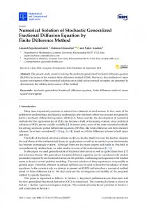
Fig. 1. Comparison between the exact solution, FDTM solution and the GL solution of (2) for T = 10, K = 8 and h = 0.01 when w(α) be Case 1.
(20)
subject to initial conditions Y0 (0) = υ1 , Y1 (0) = 0, . . . , YM −1 (0) = 0 YM (0) = υ2 , YM +1 (0) = 0, . . . , YN −2 (0) = 0 YN −1 (0) = 0.
(21) Therefore, according to differential transform method the K-term approximations for (13) can be expressed as y(t) ≈ y0 (t) =
K X
i
Y0 t M .
(22)
i=1
IV. E XAMPLE In this section, we present some examples to illustrate the efficiency of the methods. In the following, five different cases of the weighting function Rof order are discussed respectively. 1 w(α) Case 1: c Dt y(t) = 0 δ(α − 21 ) c Dtα y(t) dα and a = b = c = 1, with the initial conditions y(0) = 0,
0
y (0) = 0
Fig. 2. Comparison between the exact solution, FDTM solution and the GLM solution of equation (2) for T = 10, K = 8 and h = 0.01 when w(α) be Case 2. w(α)
c 3: Dt y(t) R 2Case 1 3 c α ) + δ(α − 1) + δ(α − Dt y(t) δ(α − 2 2) 0 a = b = c = 1, with the initial conditions
y(0) = 0,
where f (t) = t3 + 6t +
3.2t2.5 Γ(0.5)
and the exact solution is y(t) = t3 . The obtained numerical result by means of the proposed FDTM solution, GLM solution and exact solution are shown in Fig. 1, with the final time T = 10, K = 8 and h = 0.01 be Case 1. R 2 when w(α) 3 c α c w(α) Case 2: Dt y(t) = 0 δ(α − 2 ) Dt y(t) dα and a = b = c = 1, with the initial conditions y(0) = 0,
0
y (0) = 0
f (t) = t2 + 2 +
4t0.5 Γ(0.5)
and the exact solution is y(t) = t2 . Fig.2 presents a comparison of the numerical solutions FDTM, GLM and the exact solution by step size h = 0.01, K = 8 and T = 10 when w(α) be Case 2.
0
y (0) = 0
where f (t) = t3 + 3t2 + 6t +
3.2t2.5 8t1.5 + Γ(0.5) Γ(0.5)
and the exact solution is y(t) = t3 . Comparison of numerical results with the exact solution is shown in Fig. 3 by step size h = 0.01, K = 8 and T = 10 when w(α) be Case 3. R1 w(α) c Case 4: c Dt y(t) = 0 6α(1 − α) Dtα y(t) dα and a = 1, b = 0.5, c = 1.5, with the initial conditions y(0) = 0,
where
= dα and
0
y (0) = 0
where f (t) = 8. We show the numerical solutions in Fig. 4 with step size h = 0.01, H = 0.25, T = 10 and K = T /h when w(α) be Case 4.
AMINIKHAH et al.: NUMERICAL SOLUTION OF THE DISTRIBUTED-ORDER · · ·
5
We show the numerical solutions in Fig.5 with step size h = 0.01, H = 0.25, T = 10 and K = T /h when w(α) be Case 4. V. C ONCLUSION
Fig. 3. Comparison between the exact solution, FDTM solution and the GLM solution of (2) for T = 10, K = 8 and h = 0.01 when w(α) be Case 3.
In this paper, two schemes for the distributed-order BagleyTorvik equation with respect to the nonnegative density function have been described. First, by approximating the integral term in the distributed-order equation using the composite Boole’s rule, we obtained a multi-term time-fractional equation. Afterwards, the multi-term time-fractional differential equation is solved by the Grunwald-Letnikov method and the fractional differential transform method. Eventually, five examples of distributed-order Bagley-Torvik equation are presented to illustrate the efficiency and reliability of the methods. All numerical results are obtained using MATLAB 7.11. R EFERENCES [1] A. A. Kilbas, H. M. Srivastava, and J. J. Trujillo, Theory and Applications of Fractional Differential Equations. Amsterdam: Elsevier Science Limited, 2006. [2] I. Podlubny, Fractional Differential Equations. San Diego: Academic Press, 1999. [3] E. Reyes-Melo, J. Martinez-Vega, C. Guerrero-Salazar, and U. OrtizMendez, “Application of fractional calculus to the modeling of dielectric relaxation phenomena in polymeric materials,” J. Appl. Polym. Sci., vol. 98, no. 2, pp. 923−935, Oct. 2005. [4] R. Schumer, D. A. Benson, M. M. Meerschaert, and S. W. Wheatcraft, “Eulerian derivation of the fractional advection-dispersion equation,” J. Contam. Hydrol., vol. 48, no. 1−2, pp. 69−88, Mar. 2001. [5] M. Caputo, Elasticit`a e dissipazione. Bologna: Zanichelli, 1969.
Fig. 4. GLM solution and FDTM solution of the distributed-order equation (2) for T = 10, h = 0.01, H = 0.25 and K = T /h when w(α) be Case 4.
[6] M. Caputo, “Mean fractional-order-derivatives differential equations and filters,” Annali dellUniversit`a di Ferrara, vol. 41, no. 1, pp. 73−84, Jan. 1995. [7] R. L. Bagley and P. J. Torvik, “On the existence of the order domain and the solution of distributed order equations-Part I,” Int. J. Appl. Math., vol. 2, no. 7, pp. 865−882, Jan. 2000. [8] R. L. Bagley and P. J. Torvik, “On the existence of the order domain and the solution of distributed order equations-Part II,” Int. J. Appl. Math., vol. 2, no. 8, pp. 965−988, Jan. 2000. [9] M. Caputo, “Linear models of dissipation whose Q is almost frequency independent-II,” Geophys. J. Int., vol. 13, no. 5, pp. 529−539, May 1967. [10] M. Caputo, “Distributed order differential equations modelling dielectric induction and diffusion,” Fract. Calc. Appl. Anal., vol. 4, no. 4, pp. 421−442, Jan. 2001. [11] H. S. Najafi, A. Refahi Sheikhani, and A. Ansari, “Stability analysis of distributed order fractional differential equations,” Abstr. Appl. Anal., vol. 2011, Article ID 175323, Jul. 2011. [12] H. Aminikhah, A. Refahi Sheikhani, and H. Rezazadeh, “Stability analysis of distributed order fractional Chen system,” Scient. World J., vol. 2013, Article ID 645080, Oct. 2013.
Fig. 5. GLM solution and FDTM solution of the distributed-order (2) for T = 10, h = 0.01, H = 0.25 and K = T /h when w(α) be Case 5.
R1 w(α) Case 5: c Dt y(t) = 0 Γ(4 − α) c Dtα y(t) dα and a = 1, b = 2, c = 0.5, ith the initial conditions y(0) = 0,
0
y (0) = 1
where f (t) = −3t3 + 2.
[13] K. Diethelm, and N. J. Ford, “Numerical analysis for distributedorder differential equations,” J. Comput. Appl. Math., vol. 225, no. 1, pp. 96−104, Mar. 2009. [14] J. T. Katsikadelis, “Numerical solution of distributed order fractional differential equations,” J. Comput. Phys., vol. 259, pp. 11−22, Feb. 2014. [15] Z. Jiao, Y. Q. Chen, and I. Podlubny, Distributed-Order Dynamic Systems: Stability, Simulation, Applications and Perspectives. London: Springer, 2012. [16] P. J. Torvik and R. L. Bagley, “On the appearance of the fractional derivative in the behavior of real materials,” J. Appl. Mech., vol. 51, no. 2, pp. 294−298, Jun. 1984.
6
IEEE/CAA JOURNAL OF AUTOMATICA SINICA
[17] R. L. Bagley and J. Torvik, “Fractional calculus-a different approach to the analysis of viscoelastically damped structures,” AIAA J., vol. 21, no. 5, pp. 741−748, May 1983. [18] G. Boole, A Treatise on the Calculus of Finite Differences. London: MacMillan and Company, 1880. [19] X. Cai and F. Liu, “Numerical simulation of the fractional-order control system,” J. Appl. Math. Comput., vol. 23, no. 1−2, pp. 229−241, Jan. 2007. [20] A. Arikoglu and I. Ozkol, “Solution of fractional differential equations by using differential transform method,” Chaos Soliton. Fract., vol. 34, no. 5, pp. 1473−1481, Dec. 2007. [21] Z. Odibat, M. Momani, and V. S. Ertuk, “Generalized differential transform method: application to differential equations of fractional order,” Appl. Math. Comput., vol. 197, no. 2, pp. 467−477, Apr. 2008. [22] I. Petras, Fractional-order Nonlinear Systems: Modeling, Analysis and Simulation. Berlin Heidelberg: Springer-Verlag, 2011. [23] K. Diethelm and N. J. Ford, “Multi-order fractional differential equations and their numerical solution,” Appl. Math. Comput., vol. 154, no. 3, pp. 621−640, Jul. 2004.
Hossein Aminikhah received a Ph. D. degree in applied mathematics (numerical analysis) from the University of Guilan, Rasht, Iran, in 2008, where he is currently associate professor in the Department of Applied Mathematics. His research interests include numerical methods for functional differential equations and numerical linear algebra. Corresponding author of this paper.
Amir Hossein Refahi Sheikhani earned his Ph. D. (2010) from University of Guilan in Iran. He is currently an assistant professor in the Department of Applied Mathematics, Faculty of Mathematical Sciences, Islamic Azad University of Lahijan, Iran. He has authored more than 30 international refereed journal articles. His research interests include stability analysis, numerical linear algebra and optimization algorithm.
Tahereh Houlari received her B. Sc. degree in applied mathematics (2009) and her M. Sc. degree in applied mathematics (2012), from the Damghan University, Iran. She is a second-year Ph.D. student at University of Guilan, Iran. She is mainly interested in working on numerical solution of inverse problems and fuzzy logic.
Hadi Rezazadeh earned his Ph. D. (2016) from University of Guilan in Iran. He has authored more than 14 international refereed journal articles. His interests and research areas include stability analysis, numerical methods for fractional differential equations and exact solution.