Numerical study of gas-solid flow in a cyclone separator - CFD

Third International Conference on CFD in the Minerals and Process Industries CSIRO, Melbourne, Australia 10-12 December 2003

NUMERICAL STUDY OF GAS-SOLID FLOW IN A CYCLONE SEPARATOR 1

1

1

2

2

B. WANG , D. L. XU , G. X. XIAO , K. W. CHU and A. B. YU

1. School of Materials Science and Engineering, Xi’an University of Architecture and Technology, Xi’an 710055, P. R. China 2.

Centre for Simulation and Modelling of Particulate Systems, School of Materials Science and Engineering, University of New South Wales, Sydney, NSW 2052, Australia

ABSTRACT INTRODUCTION

This paper presents a numerical study of the gas-powder flow in a typical Lapple cyclone. The gas flow is obtained by the use of the Reynolds stress model. The resulting pressure and flow fields are verified by comparison with the measured results and then used in the determination of powder flow that is simulated by the use of a Stochastic Lagrangian model. The separation efficiency and trajectories of particles from the simulation are shown to be comparable to those observed experimentally. The effects of particle size and gas velocity on the separation efficiency are quantified and the results are shown to agree well with experiments.

Gas cyclone separators are widely used in industries to separate dust from gas streams or for product recovery because of its geometrical simplicity, relative economy in power consumption and flexibility with respect to high temperature and pressure. The conventional method of predicting the flow field and the collection efficiency of cyclone separator is empirical. During the past decades, application of computational fluid dynamics (CFD) for the numerical calculation of the gas flow field in a cyclone is becoming more popular. One of the first CFD simulations was done by Boysan [1]. He found that the standard k − ε turbulence model is inadequate to simulate flows with swirl because it leads to excessive turbulence viscosities and unrealistic tangential velocities. Recent studies suggest that the accuracy of numerical solution can be improved by using Reynolds Stress Model (RSM) [2-4].

NOMENCLATURE CD d Fk g p' rp Re t u u′

drag coefficient particle diameter, m the momentum transport coefficient, t-1 acceleration due to gravity, m s-2 dispersion pressure, Pa radius of particle, m Reynolds number time, s instantaneous velocity, m s-1 dispersion velocity, m s-1

u u

p

time average velocity in axial direction, m s-1 particle instantaneous velocity in axial direction,

p

m s-1 particle instantaneous velocity in radial direction,

v

Currently, particle turbulent dispersion due to interaction between particles and turbulent eddies of fluid is generally dealt with by two methods [5]: mean diffusion which characterizes only the overall mean (time-averaged) dispersion of particles caused by the mean statistical properties of the turbulence, and structural dispersion which includes the detail of the non-uniform particle concentration structures generated by local instantaneous features of the flow, primarily caused by the spatialtemporal turbulent eddy features and evolutions. For prediction of the mean particle diffusion in turbulent flow, both Lagrangian and Eulerian techniques can be used. The stochastic Lagrangian model employs a stochastic sampling approach to simulate the turbulent fluctuations of the fluid at particle location. Since the early work of Yuu et al. [6] and Gosman and Ioannides [7], the stochastic Lagrangian model has shown significant success in describing the turbulent diffusion of particles. It has been reported that it is necessary to trace up to 3×105 particle trajectories in order to achieve statistically significant solutions even for two-dimensional flows [8,9]. In order to bring Stochastic Lagrangian model into industrial applications, some modified models were proposed. Sommerfeld et al. [10] proposed Langevin stochastic differential equation models by making use of Possibility Density Function (PDF). Litchford and Jeng [11] developed a stochastic dispersion-width transport model, where the dispersion-width is explicitly computed through the linearized equation of motion using the concept of particle-eddy interactions. Moreover, Chen and

m s-1

v w

p

time average velocity in radial direction, m s-1 particle instantaneous velocity in tangential direction, m s-1

w x δ µ

ρ

time average velocity in tangential direction, m s-1 axis, m Kronecker factor fluid viscosity, kgm-1 s-1 density, kg m-3

SUBSCRIPTS g i ,j,k p

gas 1,2,3 particle

Copyright  2003 CSIRO Australia

371

of fluid and the drag force caused by dispersion velocity of fluid. Then the momentum equation of a particle in the two phase flow with ambient temperature can be expressed as:

Pereira [12] reported a SPEED model where a combined stochastic-probabilistic method is used to describe the turbulent motion of discrete particles so that only a small number of particle trajectories is required. In this paper, we used RSM and Stochastic Lagrangian model in Fluent to study the gas-solid flow in a typical Lapple cyclone separator. The model is verified by comparing the simulated and measured results in term of gas pressure and flow fields, solid flow pattern and collection efficiency. The effects of particle size and gas velocity are discussed.

du

dv

k

k

)

(

k

)

w

(2)

2 p

(3)

r

p

dw p dt

There are usually three models used in cyclone simulation: k − ε model, algebraic stress model (ASM) and RSM. The k − ε model adopts the assumption of isotropic turbulence, so it is not suitable for the flow in cyclone which has anisotropic turbulence. ASM can not predict the recirculation zone and Rankine vortex in strongly swirling flow since it ignores or underestimates the effect of stress convection. RSM forgoes the assumption of isotropic turbulence and solves a transport equation for each component of the Reynolds stress. It is thought as the most applicable turbulence model for cyclone flow field even though it has the disadvantage of being more computationally expensive than other unresolved-eddy turbulence models [2-4].

p

= F v + v′ − v +

p

dt

MODEL DESCRIPTION

(

= F u + u′ − u − g

p

dt

(

F =

where

)

= Fk w + w′ − w 2p −

k

Re 18µ C 24 d ρ

is

p

D

2

p

v p wp

(4)

rp

the momentum transport

p

coefficient between fluid and particles, and the drag coefficient is given as:

24   Re   24 1 + 0 .15 Re C = Re  0 .44   

(

0 .687 p

Re ≤ 1 p

)

1 < Re ≤ 1000

D

p

p

where Re =

Re > 1000 p

d ρ ϕ −ϕ p

g

p

is the Particle Reynolds

g

µ

p

In RSM, the transport equation is written as [13]:

number, φ can be u , v and w . When the particle p

interacts with fluid eddy, u ′

j

k

i

j

ij

ij

ij

ij

where the left two terms are the local time derivative of stress and convective transport term, respectively. The right five terms are: the stress diffusion term:

SIMULATION CONDITIONS

    ρ u ′u ′u ′ +  p′u′ δ +  p′u′ δ − µ  ∂ u′u′   ∂x i j   i j k  j  ik  i  jk     k 

003  fluent6.0.12

De

S

b

the shear production term: h

  

a

H

the pressure-strain term : Π = p′( ij

the dissipation term: ε = −2µ

′ ∂u ′ ∂u i + j ) ∂x j ∂xi

D

 ∂u j ∂u i + u ′j u k′ Pij = − ρ u i′u ′k ∂x k ∂x k 

ij

v′

standard deviation of 2k / 3 . Particle-eddy interaction time and dimension should not be larger than the lifetime and size of a random eddy.

k

∂ D =− ij ∂x k

、 、 p

w′ is obtained by sampling from an isotropic Gaussian distribution with a

∂ ∂ ′ ′ ′ ′ (ρ u u ) + ( ρu u u ) = D + P + Π − ε + S (1) ∂t ∂x i

p

′ ′ ∂u i ∂u j ∂x k ∂x k

B

(a)

(b)

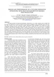
and the source term: S Figure 1. Schematic and grid representation of the cyclone.

In the modelling of particle dispersion, the interactions between particles are neglected since only dilute flow is considered in this model. The virtual mass force, the Basset force, the Magnus force and the Saffman force are not considered. Only the gravity force and gas drag force on particles are calculated. The gas drag force is decomposed as the drag force caused by average velocity

Figure 1(a) shows the notations of the cyclone dimensions and Table 1 indicates the dimensions of the typical Lapple cyclone. Figure 1(b) shows the computational domain, containing 45750 CFD cells. The whole computational domain is divided by structured hexahedron grids. At the

372

zone near wall and vortex finder the grids are dense, while at the zone away from wall the grids are sparse. The gas pressure at the top of the vortex finder is 1 atm. Unless otherwise specified, the inlet gas velocity and the particle velocity are both 20m/s.

Dynamic Pressure 501.993 478.695 455.397 432.099 408.801 385.503 B 362.205 338.907 315.609 292.311 269.013 245.716 222.418 199.12 175.822 152.524 129.226 105.928 82.6298 59.3319 36.0339 12.736

B

Physical experiment has also been conducted to validate the numerical model. The particles used are the cement raw materials. The particle size distribution can be well described by the Rosin-Rammler equation, with the characteristic diameter equal to 29.90µm and the distribution parameter 0.806. The particle density is 3320kg/m3.

Table 1. Geometry of the cyclone considered (D =0.2m) a/D

b/D

De/D

S/D

h/D

H/D

B/D

0.5

0.25

0.5

0.625

2.0

4.0

0.25

A

A

A-A

B-B

Figure 3. Contour of dynamic pressure

5500 5000

Numerical Experimental

4500

RESULTS AND DISCUSSION

) 4000 aP ( 3500 po rd 3000 2500 er us 2000 se 1500 r P 1000

Gas flow field Figure 2 shows that the static pressure decreases radially from wall to centre, and a negative pressure zone appears in forced vortex. This means there is a negative pressure zone in the center of the cyclone. The black line in Figure 2 is the dividing line between the positive static pressure and negative static pressure. The pressure gradient is the largest along radial direction, as there exists a highly intensified forced vortex.

500 0

B

A-A

15

20

25

30

35

Figure 4. Experimental results of pressure drop compared with calculated results Figure 4 shows the relation between the pressure drop and the inlet gas velocity. With the increase of the inlet gas velocity, the pressure drop increases. The experimental data obtained agree reasonably well with the calculated results although consistently slightly higher. 28 26

A

A

24 22

Tangential Velocity (m/s)

B

10

The inlet gas velocity(m/s)

Static Pressure 845.024 798.656 715.192 671.915 619.363 542.082 498.805 440.071 368.973 325.695 260.779 195.863 152.585 81.4867 22.7531 -8.15939 -63.8018 -107.079 -187.452 -236.912 -280.189 -366.744

5

B-B

20 18 16 14 12 10

experimental numerical

8 6 4 2

Figure 2. Contour of static pressure

0 -0.10

Figure 3 shows that the dynamic pressure is the largest in the CS surface (the interface between forced vortex and quasi-free vortex). In the quasi-free vortex zone, the dynamic pressure increases with the radius while the dynamic pressure decreases and tends to zero in the forced vortex zone. Figure 3 shows that the distribution of dynamic pressure is asymmetrical due to the nonsymmetry of the tangential velocity.

-0.08

-0.06

-0.04

-0.02

0.00

0.02

0.04

0.06

0.08

0.10

X ( m)

Figure 5. Experimental results of tangential velocity compared with calculated results Figure 5 shows the experimental and calculated tangential velocities at the cylindrical section of the cyclone. The simulation results are in good agreement with the experimental results. The flow field in cyclone indicates the expected forced/free combination of the Rankine

373

vortex finder will help weaken the chaotic flow and reduce pressure drop. Figure 7 also shows the diameter of forced vortex is a little larger than that of the vortex finder. Moreover, since much gas flow inbursts the vortex finder, the axial velocity reaches a peak value when gas flow into the vortex finder.

vortex. Moreover, because the cyclone has only one gas inlet, the axe of the vortex does not coincide with the axe of the geometry of cyclone. Figure 6 shows the calculated tangential velocity distribution in detail. The tangential velocity distribution is similar to the dynamic pressure distribution. This means the tangential velocity is the dominant velocity in cyclone. The value of tangential velocity equals zero on the wall and the centre of the flow field. The high speed gas enters the inlet and is accelerated up to 1.5~2.0 times of the inlet velocity at point A. Then the velocity decreases as the gas spins down along the wall. Before it goes below the vortex finder, the gas flow collides with the follow-up flow and forms a chaotic flow close to the vortex finder outside wall (B point). The gas velocity decreases sharply at point B. This is the main cause of the short-circuiting flow and often results in a high pressure drop. Tangential Velocity 29.4518 27.5895 25.7272 C 23.8649 22.0025 20.1402 18.2779 B 16.4155 14.5532 12.6909 10.8286 8.96624 7.10391 5.24158 3.37925 1.51693 -0.3454 -2.20773 -4.07005 A -5.93238 -7.79471 -9.65704

C

B

A-A

From Figure 8 (A-A), we can see that the forced vortex in the central is a twisted cylinder. The axis of the forced vortex is not coincided at the geometrical axis of cyclone, and also is not a line but a curve. There is a zone right under the vortex finder where gas flows into the vortex finder directly instead of spinning down to the conical section and then flowing upward. This is the shortcircuiting flow, which does harm to cyclone performance. In the conical section, the radial velocity is much larger than that of cylinder section. This will drag some particles into the forced vortex and these particles will not be collected. From Figure 8 (B-B), we see that the distribution of radial velocity is nearly uniform in the quasi-free vortex area. The distribution of the radial velocity in the forced vortex is eccentric because of the non-symmetrical geometry of the cyclone. Figure 8 (C-C) shows that the radial velocity is negative or inward flow in the gas inlet and then becomes zero rapidly. Afterwards it becomes positive due to the effect of centrifugal force around the vortex finder. At point A, the radial velocity becomes negative again, directing to the centre, because of the collision among gas.

A

B

C-C

A

B-B

C

C

B

B

Radial Velocity 6.16873 5.29714 4.86135 4.3633 3.55397 3.11817 2.55787 1.81079 1.375 0.752432 0.0676124 -0.368182 -1.053 -1.67557 -2.11136 -2.85844 -3.41874 -3.85454 -4.66387 -5.16192 -5.59771 -6.4693

Figure 6. Contour of tangential velocity

Axial Velocity

B

B

A-A

21.4941 19.9052 18.3163 16.7274 15.1385 13.5496 11.9607 10.3718 8.78294 7.19405 5.60515 4.01625 2.42736 0.838464 0 -1.54488 -3.13377 -4.72267 -6.31157 -7.90046 -9.48936 -11.0783

A

A C-C A

A

A

A-A

B-B

Figure 8. Contour of redial velocity distribution

Particles flow pattern Figure 9 shows the change in location with time of 15000 particles with five diameters within 1 second. Red, orange, green cyan and blue respectively represent five diameters of particles, that is, 1 10-4m, 3 10-5m 7 10-6m, 2 10-6m and 2 10-7m. From this figure, it can be seen that the trajectory of the largest particles (red) is at the upside of the cone, the trajectory of the smallest particles (blue) is at the downside of the cone. The other three sized particles are largely in-between the two extremes.

B-B

Figure 7. Contour of axial velocity Figure 7 shows that the forced vortex is a twisted cylinder and not completely axially symmetric, especially in the conical section. From Figure 7 (B-B) we see the centre of the forced vortex dose not coincided with the geometrical centre of cylindrical body of the cyclone, which deflected to the gas inlet. This should be one of the main reasons why there is eccentric vortex finder in some revised cyclone separators and some modified inlet shapes were proposed [14]. From Figure 6 (C-C), we see eccentric

×

374

×

×

，×

×

There is therefore a critical value to distinguish the flow pattern of particles of different diameters. If the particle diameter is larger than the critical value, the particle will keep a circular motion in the cone of cyclone. In contrast, if the particle diameter is less than this critical value, the particles will be collected directly or escape from the cyclone. The critical value is related to the geometry of cyclone, the gas inlet velocity and the properties of particles. In this cyclone, the critical diameter is approximately 1 10-5m.

×

t=0.05s

t=0.1s

t=0.15s

t=0.2s

t=0.3s

t=0.35s

t=0.4s

t=0.45s

In order to verify the numerical simulation results, physical experiments have been done by use of two types of ceramic balls whose density is similar to the cement raw material. The diameter of yellow ceramic ball is 1mm, and the green ones are 2mm. The experimental results are shown in Figure 10. In Figure 11 (a), the pure cement raw material was used. It is observed that the particles flow downward at the cone section and display a certain descending angle. On the other hand, ceramic ball (Figure11-b) kept spinning at a certain height and did not show the descending angle. This phenomenon supported the simulation results. In the real industry, these bigger particles will be eventually collected due to their interactions with other particles.

t=0.25s

t=0.5s

2 t=0.55s

t=0.6s

t=0.8s

t=0.85s

t=0.65s

t=0.9s

t=0.7s

t=0.75s

t=0.95s

t=1.0s

×10 m 2×10 m 7×10 m 3×10 m 1×10 m -7

-6

-6

-5

-4

Figure 10. The trajectories of particles with different diameters

Figure 9. Animation of particle flow As shown in figure 9, large particles are collected while small particles escape from the cyclone. The particles with the smallest diameter can not move outward to the wall of cyclone since the centrifugal force on them is not bigger than the gas drag force on them. The particles with diameters of 2 10-6m and 7 10-6m can spin down to the conical section of cyclone and then should be collected while the bigger particles with diameter of 3 10-5m and 1 10-4m spin downward first and then keep spinning near the wall at a certain horizontal level.

×

×

×

a

b

Figure 11. Photos showing the trajectories of tracing particles of different diameters

×

375

100

6.

Separation efficiency ( % )

98

5.

LOTH E., “Numerical approaches for motion of dispersed particles, droplets and bubbles”, Progress in Energy and Combustion Science 26 (2000) 161223.

6.

YUU S., YASUKOUCHI N., HIROSAWA, “Particle turbulent diffusion in a dust laden round jet”, AIChE Journal 24 (1978), 509-519.

7.

GOSMAN A.D. and IOANNIDES E., “Aspects of computer simulation of liquid-fuelled combustors”. AIAA 19th Aerospace Science Mtg., Paper 81-0323 (1981) St. Louis, Mo..

8.

STURGESS G.J., SYED S.A., “Calculation of a hollow-cone liquid spray in uniform airstream”. Journal of Propulsion and Power, 1 (1985) 360-369.

9.

MOSTAFA A.A., MONGIA H.C., MCDONELL, V.G. and SAMUELSEN, G.S., “Evolution of particle-laden jet flows: a theoretical and experimental study”, AIAA Journal, 27 (1989)167183.

96 94 92 90 88 86

Numerical Experimental

84 82 80 0

2

4

6

8

10 12 14 16 18 20 22 24 26 28 30 32 34

Inlet gas velocity(m/s)

Figure 11. Experimental results of separation efficiency compared with calculated results The most important economical parameters of a cyclone separator are separation efficiency and pressure drop. Generally, The increase of gas inlet velocity will increase the separation efficiency, but it will also increase the pressure drop. In this work, physical and numerical experiments have both been done to find the effect of gas inlet velocity on separation efficiency and pressure drop. As shown in Fig. 4, the pressure drop increases with the inlet gas velocity, and there is a good agreement between predicted and measured results. Figure 11 shows that the collection efficiency can be enhanced with the increase of inlet gas velocity, as expected. The prediction matches the measurement reasonably well.

10. SOMMERFELD M, KOHNEN G and RUGER M. “Some open questions and inconsistencies of Lagrangian particle dispersion models”, Proc. Ninth Symp. on Turbulent Shear Flows, Kyoto, Japan, Paper (1993) . 11. LITCHFORD R.J. and JENG SM, “Efficient statistical transport model for turbulent particle dispersion in sprays”. AIAA Journal 29 (1991) 1443-1451.

CONCLUSIONS

12. CHEN XQ, PEREIRA JCF, “Efficient computation of particle dispersion in turbulent flows with a stochastic-probabilistic model”, Int. J. Heat and Mass Transfer, 40 (1997) 1727-1741,.

RSM has been used to simulate the anisotropic turbulence flow in a Lapple cyclone. Its applicability has been verified by the good agreement between the calculated and measured pressures and flow fields. On this basis, a stochastic Lagrangian model has been used to predict the flow pattern of particles in the cyclone and its validity is confirmed by comparing the predicted and measured solid flow trajectories and collection efficiency. The proposed model provides a convenient way to study the effects of variables related to operational conditions, cyclone geometry and particle properties, which is important to the optimum design and control of cyclone process.

13. SHUN R. and LI Z.Q., “Simulation of strong swirling flow by use of different turbulence model”, Power Engineering 22 (2002). 14. SUASNABAR, D. J., “Dense medium cyclone performance enhancement via computational modelling of the physical processes”, Ph.D thesis (2000).

REFERENCES 1.

BOYSAN F, AYER WH, SWITHENBANK JA, “Fundamental mathematical-modeling approach to cyclone design”, Transaction of Institute Chemical Engineers, 60 (1982) 222-230.

2.

HOEKSTRA A.J., DERKSEN J.J., H.E.A. VAN DEN AKKER “An experimental and numerical study of turbulent swirling flow in gas cyclones”, Chemical Engineering Science 54 (1999) 2055-2056.

3.

PANT K., CROWE C.T., IRVING P., “On the design of miniature cyclone for the collection of bioaerosols”, Powder Technology 125 (2002) 260265

4.

SOMMERFELD M., HO C. H., “Numerical calculation of particle transport in turbulent wall bounded flows”, Powder Technology 131 (2003) 1-

376