Numerically Optimized Empirical Modeling of Highly Dynamic, Spatially Expansive, and Behaviorally Heterogeneous Hydrologic Systems – Part 1 Edwin Roehl, Advanced Data Mining, Greer South Carolina,
[email protected] John Risley, U.S. Geological Survey, Portland Oregon,
[email protected] Jana Stewart, U.S. Geological Survey, Middleton Wisconsin,
[email protected] Matthew Mitro, Wisconsin DNR, Madison Wisconsin,
[email protected]
Abstract: Natural systems exhibit random, chaotic, and multiply periodic behaviors that are driven by gravity, weather, and man-made disturbances. Modeling them on a large scale is challenging because behaviors vary discontinuously both spatially and in time. Modeling requires calibration and validation data that represent a diversity of causes and effects. Measured variables are either categorical (static) or dynamic (time series). Integrating multiple data types and reducing large numbers of variables to a select set often leads to subjective decision-making that has significant ramifications when applying state-of-the-art multi-step modeling approaches, e.g., land-use models driving finite element flow models. This paper is Part 1 of a two-part treatment that describes an alternative approach that employs a sequence of numerically optimized data mining algorithms. They include 1) signal decomposition to separate static, chaotic and periodic time series components that are attributable to different forcing functions; 2) time series clustering to segment monitored sites by their dynamic behaviors; 3) non-linear, multivariate sensitivity analysis using multi-layer perceptron artificial neural networks (ANN) to determine the relative importance of categorical variables at predicting site-to-site behavioral variability; 4) spatially interpolating dynamic behaviors with ANNs; and 5) assembling an end-user application that integrates data, site attribute classifiers, and prediction models to model an expansive, behaviorally heterogeneous natural system. This paper also describes applications of this approach that predict water levels and stream temperatures. Keywords: clustering; classification; neural network; model
1. INTRODUCTION Natural resource managers commonly ask scientists to create predictive models of spatially expansive natural systems for planning their protection or management. This involves collecting old and new data for model development. The data should come from multiple locations that represent the diversity of behaviors across the natural system. Measured variables are either categorical (static), e.g., geology; infrequent time series, e.g., monthly or annually; or real-time, e.g., hourly or daily. Time series variables (signals) usually have multiply periodic behavioral components caused by the earth’s orbital motions. Periodicity is by definition highly predictable; however, signals also display dramatic spatial and temporal variability due to chaotic forcing by humans and weather.
Chaotic behaviors are by definition only somewhat predictable, yet it is these that modelers strive to reproduce. Techniques such as band-pass and window average filtering can decompose a signal to separate the periodic components, leaving behind chaotic components. A study by Conrads and Roehl [1999] found that multi-layer perceptron artificial neural network models (ANN) of the type described by Jensen [1994] offered a number of advantages over finite difference physics-based models in reproducing the dynamic flow and water quality behaviors in an estuary. Most importantly, the ANNs gave much better prediction accuracy when using the same input and output variables and data. Coppola et al [2005] made some of the same observations after applying ANNs to forecast water levels (WL) at two monitoring wells in an aquifer affected by
climatic variables and pumping. ANNs are a curve fitting technique that synthesizes continuously differentiable, multivariate non-linear functions to near-optimally fit measurements that represent complex process behavior. Being empirical, their perceived shortcomings generally result from misapplication, e.g., failure to decorrelate input variables.
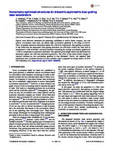
Figure 2 shows WLDi(t) for a sub-set of the wells. While an annual periodic component is apparent, there is also the dramatic year-to-year variability typical of chaotic forcing. Figure 2 also shows that well behaviors are spatially discontinuous due to differences in process physics.
A benefit of finite difference models is their ability to provide spatially semi-continuous predictions from mesh nodes. Conrads et al [2003] showed how ANN outputs for multiple locations could be interpolated as a post-processing step, and Dowla and Rogers [1996] used ANNs to represent static 3D land elevations; however, determining a method for configuring ANNs to simultaneously predict spatial and temporal variability became a research objective.
Figure 2: ≈30x50km2 detail showing well locations and hydrographs. Dotted line marks the river.
Figure 1. Well locations in ≈140x140km2 of the Suwannee River Valley. Peak elevation ≈ 75m.
2. AQUIFER WATER LEVEL A database of daily water levels WLDi(t) (i=well#) from over 200 monitoring wells in the Floridan Aquifer (Figure 1) provided an opportunity to investigate how to configure ANNs to spatially interpolate dynamic behaviors. The area’s water managers were interested in determining how to defensibly reduce the size of their monitoring network; however, the data was also used to research if an ANN model could generate spatially continuous WL predictions from static variables and WL signals.
Figure 3. Normalized WL for Classes 2 and 4. Xaxis is in days from April 1982 to October 1998. A stacked database was created for training ANNs to spatially interpolate. Each well was represented by a block of rows denoting time stamps and columns denoting candidate input and output variables. Training vectors are subsets of rows. The input and output variables and their column order were identical for all blocks. The blocks were
stacked one on top of the other. Candidate input variables, each stacked repetitiously in its own column, were either categorical (static), changing well-to-well but not in time, or time series. The only available static variables were UTM x and y, and surface elevation z (xyz). The static components of WLDi(t) at the wells were calculated, WLSi ≡ the historical mean of WLDi(t). Additional columns were created to hold the output variables to be predicted – stacked versions of WLSi and WLDi(t) that changed block-to-block according to each block’s associated well xyz. Similarly to Dowla and Rogers [1996], a static sub-model was trained to predict how WLS varied spatially with input xyz. Its output was cascaded to be an input to a chaotic sub-model that predicted how WLDi(t) varied spatially and temporally. Other inputs to the chaotic sub-model included xyz, and various WLDi(t) from different wells. The two sub-models comprised a super-model.
are generally ill suited to synthesizing discontinuous functions; a divide-and-conquer approach was needed to the segment disparate behaviors. A time series clustering algorithm was developed to subdivide wells into classes having similar behaviors. The hydrographs of all the wells were cross-correlated to produce a matrix of Pearson coefficients. Each row and column represented a different well and its behavioral similarity to each of the other wells. The rows were then clustered using the k-means algorithm. The number of classes was determined by the sensitivity of the mean square error to k. Figure 3 shows hydrographs of two of 12 classes. It is apparent that the members of a class are similar, and dissimilar to those in the other class. Not surprisingly, there were gradations of similarity class-to-class. A side benefit of time series clustering is that it identifies redundant data, largely answering the question of, “Which monitoring wells can be discontinue?” Further, measurements that are reproducible from others using a model are potentially unneeded. Sub-model pairs were developed for each class. Figure 4 shows results for two wells.
Figure 5. Grid with color-coded class assignments. Cells are 1-km2. Figure 4. Measured and predicted normalized water levels for a Class 1 well and a Class 3 well. Sub-model development is an experimental process in which different input variable combinations and ANN architectural and training parameterizations are evaluated using statistical measures of prediction accuracy. Regardless of the inputs used, it was found that a single static+chaotic sub-model pair was unable to adequately predict WLs throughout the study area. Given the behavioral discontinuities shown in Figure 2, and that ANNs
The next step was to classify regions of the study area so that the most appropriate model class would be applied to a “new” site. As shown in Figure 5, the study area was divided into 1-km2 cells. All of the cells were assigned to a class by piecewise krigging well x, y, and class codes. Figure 6 shows a snapshot of the WL surface predicted by the super-model. Averaging smoothed prediction differences at class boundary cells. Long-term simulations revealed highly asynchronous spatial and temporal variability in the water levels driven by precipitation, pumping, and surface water levels.
Figure 7 shows how the run-time application was assembled. A new site vector is passed to a classifier, which looks up the cell’s class based on x and y. The classifier instructs a control program which class’ sub-models to run. The program runs a simulation by stepping time, routing the new site static data and real-time data from a time series database to the sub-models, and logging predictions. The static sub-model’s predictions are cascaded to the chaotic sub-model. Input WLDi(t) could be modulated by the user to evaluate alternative outcomes.
4. ANN Modeling – provides near optimal multivariate non-linear curve fitting of static and dynamic variables. 5. New Site Classification – here, krigging was used to produce near-numerically optimal assignments of sites to behavioral classes. Other options include (linear) nearest neighbor and non-linear ANN classifiers. 6. Super-Model – complex modeling problems are solved with relatively simple, near-numerically optimal sub-models of optimally segmented behaviors and classified sites.
3. OREGON STREAM TEMPERATURES
Figure 6. Snapshot of super-model output. Peak elevation is approximately 60m above sea level.
Figure 7. Run-time application architecture. In summary: 1. Signal Decomposition – decomposes time series into static and dynamic components to reduce the complexity of a behavior to be modeled. This improves the accuracy of sub and super-models. 2. Time Series Clustering – produces numerically optimal segmentation of time series into behavioral classes. 3. Stacked Database – configures static and time series variables for training ANNs to spatially interpolate.
Risley et al [2003] describe how the approach was adapted to model “natural” temperatures in small streams in the western third of Oregon to support federal and state conservation initiatives. The available data were: • Stream Temperature (ST) - hourly time series from 148 “natural” sites recorded from June to September 1999 (Figure 8). The sites were located on streams that drained basins ranging from 0.3 to over 300 km2. Site elevations ranged from 7 to 1,445 m above mean sea level. Six of the 148 sites were randomly withheld from model development for validating results. • Climate – 65 hourly time series of air temperature, dew-point, solar radiation, barometric pressure, snowpack, and precipitation from 25 locations. • Stream Habitat and Basin Attributes – 34 static variables that included stream bearing, gradient, canopy cover, wetted widths, depth, and bed substrate; and basin topographic and vegetation characteristics such as size and forest cover. Differences between this and the Floridan Aquifer model included: • A need to predict hourly rather than daily ST. This indicated a need for three sub-models for each behavioral class to predict static, chaotic, and hourly STs. An attempt to model daily maximums directly was less successful than modeling the hourly ST and picking them out, suggesting that it might be better to create the best possible process model and use it to compute statistics of interest. • A large list of candidate static and dynamic inputs whose interrelationships and predictive performance were unknown. Many of the variables were highly correlated.
• New site classification could not be based solely on spatial coordinates because of the influences of habitat and basin attributes. Thus, the space to be interpolated was an “abstract” space defined by the static variable model inputs.
calculating differences from the standard at the other stations.
Figure 8. Western Oregon study area. Class 1, 2, and 3 sites are circles in white, gray, and black respectively. Triangles mark climatic and snowpack monitoring sites. Signal decomposition of the hourly water temperature time series STHi(t) involved the following. The static components at the sites STSi ≡ the historical mean of STHi(t). The chaotic components STCi(t) ≡ the 24-hour moving window averages of STHi(t). STCi(t) was then normalized as STCNi(t) = STCi(t) – STSi. STHi(t) was normalized as STHNi(t) = STHi(t) – STCNi(t) - STSi. STCi(t) were clustered into three classes using time series clustering. Class 1 sites were generally located in warmer climate regions at lower elevations and in the southern portion of the study area. This includes the Klamath Mountains ecoregion and the Willamette River valley lowlands. Class 2 sites were more predominant at higher elevations, particularly in the Cascade Mountains. Class 3 sites were widely distributed at middle elevations. The climatic hourly time series, generically CHi(t), were decomposed into chaotic components CCi(t) ≡ 24-hour moving window averages of CHi(t), and normalized hourly CHNi(t) = CHi(t) – CCi(t). Each type of climatic variable was measured at multiple stations. These tended to be highly correlated station-to-station, so they were decorrelated by setting one station to be a “standard” and
Figure 9. Measured and predicted STs at two validation sites. A single static sub-model that used only static variable inputs to interpolate STS for all three classes was used. For each class, chaotic submodels were trained to interpolate STCNj(t) from static and chaotic climatic inputs. Similarly, hourly sub-models were trained to interpolate STHNj(t) from static and hourly climatic inputs. Input variables were selected according to their predictive performance. STHi(t) and STCi(t) predictions were summations of the static and normalized chaotic and hourly predictions. The critical input variables included air temperature, riparian shade, site elevation, and basin percent forested area. Figure 9 shows measured and predicted STHi(t) at the “best” and “worst” of the six validation sites. Both predictions track the climatically-forced dynamic behaviors; however, the Fisher Creek predictions are offset from the measurements by an average of 2.4 C. The offset is due largely to the error in the predicted static ST, suggesting that overall model error is a consequence of the process by which habitat and basin attributes are determined. A second explanation is the procedure
used to select validation sites, e.g., random selection as was used here. A validation site whose attributes are unique and unlearned will be poorly represented by an empirical model.
same type was met by setting one station to be a “standard” and calculating differences from the standard at the other stations. A non-linear new site classifier was developed using ANNs.
A non-linear classifier comprised of three ANNs, one for each class, was created to select the appropriate static+chaotic+hourly sub-model triplet for a new site. Each class’ ANN was trained to predict a binary 0 or 1 depending if a new site’s habitat and basin attributes matched those of its member sites. Programmed logic was used to resolve ambiguous cases.
Outstanding issues include how to non-linearly decorrelate variables of different types; selecting validation sites with an understanding of their relative uniqueness; and architecting, training, and interpreting multi-layer perceptron ANNs. Part 2 will address these issues while describing the development of another application with a major and unfortunately common twist. A model of STs for the entire state of Wisconsin was developed for managing fisheries. It was similar to the Oregon ST model, except the available ST time series from 254 sites were temporally scattered over a dozen summers. Few sites overlapped year-to-year making time series clustering problematic.
4. CONCLUSIONS This first of a two-part treatment provides an overview of a divide-and-conquer approach to empirically model spatially heterogeneous, dynamic behaviors. These behavior are described by many types of categorical and time series data that should be used to the fullest possible extent. And, it is very important to avoid making subjective decisions about which data is important. The Floridan Aquifer exhibited not only highly disparate behaviors well-to-well, but also gradations of these behaviors. Time series clustering provided a numerically optimal solution to segmenting the wells into classes. Krigging class assignments was a numerically optimal means to classify sites between the wells. ANNs use an inherently non-linear, multivariate architecture and error minimizing training algorithms to fit data representing complex behaviors. Their performance is improved by decomposing time series into static and dynamic components and modeling them separately. Modeling behavioral classes separately avoids prediction errors caused by fitting discontinuous behaviors with continuous functions. ANNs can be trained to spatially interpolate with a stacked training database that combines static and time series variables. The best predictor variables can be found by systematically adding and removing candidates and tracking statistical measures of prediction accuracy. ANN sub-models are easily assembled into super-models that can be integrated with a database and control program to form run-time application. Modeling Oregon STs extended the approach. Dozens of non-spatial site attributes and climatic time series from multiple stations were used. The need to decorrelate climatic input variables of the
5. REFERENCES Conrads, P.A., and E.A. Roehl, Comparing physicsbased and neural network models for predicting salinity, water temperature, and dissolved-oxygen concentration in a complex tidally affected river basin, paper presented at the South Carolina Environmental Conference, Myrtle Beach, March 15-16, 1999. Conrads, P.A., E.A. Roehl, and W.P. Martello, Development of an empirical model of a complex, tidally affected river using artificial neural networks,” Water Environment Federation TMDL Specialty Conference, Chicago, Illinois, November 2003. Dowla, F.U. and L.L. Rogers, Solving Problems in Environmental Engineering and Geosciences with Artificial Neural Networks, MIT Press, 159-172, Cambridge MA, 1996. Coppola, E.A., A.J. Rana, M.M. Poulton, F. Szidarovszky, and V.W. Uhl, A neural network model for predicting aquifer water level elevations, Ground Water 43(2), 231-241, 2005. Jensen, B.A., Expert systems - neural networks, Instrument Engineers’ Handbook Third Edition, Chilton, Radnor PA, 1994. Risley, J.C., E.A. Roehl and P.A. Conrads, Estimating water temperatures in small streams in western Oregon using neural network models, U.S. Geological Survey WaterResources Investigations Report 02-4218, 2003.