Nutrient uptake and net primary production

INFORMATION TO USERS

This manuscript has been reproduced from the microfilm master. UMi films the text directly from the original or copy submitted. Thus, some thesis and dissertation copies are in typewriter face, while others may be from any type of computer printer. The quality of this reproduction is dependent upon the quality of the co p y subm itted. Broken or indistinct print, colored or poor quality illustrations and photographs, print bleedthrough, substandard margins, and improper alignment can adversely affect reproduction. In the unlikely event that the author did not send UMI a complete manuscript and there are missing pages, these will be noted.

Also, if unauthorized

copyright material had to be removed, a note will indicate the deletion. Oversize materials (e.g., maps, drawings, charts) are reproduced by sectioning the original, beginning at the upper left-hand comer and continuing from left to right in equal sections with small overlaps.

ProQuest Information and Learning 300 North Zeeb Road, Ann Arbor, Ml 48106-1346 USA 800-521-0600

Reproduced with permission of the copyright owner. Further reproduction prohibited without permission.


MASS TRANSFER LIMITS TO NUTRIENT UPTAKE BY SHALLOW CORAL REEF COMMUNITIES

A DISSERTATION SUBMITTED TO THE GRADUATE DIVISION OF THE UNIVERSITY OF HAW AIT IN PARTIAL FULFILLMENT OF THE REQUIREMENTS FOR THE DEGREE OF DOCTOR OF PHILOSOPHY IN OCEANOGRAPHY DECEMBER 2002

By James L. Falter Dissertation Committee: Marlin J. Atkinson, Chairperson Carlos F.M. Coimbra Mark A. Merrifield Francis J. Sansone Stephen V. Smith


UMI Number 3070700

UMI* UMI Microform 3070700 Copyright 2003 by ProQuest Information and Learning Company. All rights reserved. This microform edition is protected against unauthorized copying under Title 17, United States Code.

ProQuest Information and Learning Company 300 North Zeeb Road P.O. Box 1346 Ann Arbor. Ml 48106-1346


We certify that we have read this dissertation and that, in our opinion, it is satisfactory in scope and quality as a dissertation for the degree of Doctor of Philosophy in Oceanography.

? / I DISSEKTATION'COMMITTEE

Chairperson

___________

f t \Al

ii Reproduced with permission of the copyright owner. Further reproduction prohibited without permission.

© Copyright (2002) by James L. Falter

iii


ACKNOWLEDGEMENTS I would like to thank my committee for all of their assistance and interaction; it was clear they were looking out for my best interests. Mahalo nui to Jim Fleming, who as an unofficial committee member and mentor, showed me how to work with my hands. His assistance in the field and in the construction of various experimental apparati (often without the benefit of calculus) was fundamental to the completion of this degree. I would like to thank Eric Hochberg for his support as a friend, sounding board, field assistant, and international dive guide. I would also like to thank Dan Hoover, Jennifer Liebeler, Janie Culp, and Ann Tarrant for the moral support that is essential for any graduate student to succeed. I would like to thank Kimball Millikan, Philippe Barrault, Serge Andrefouet, Kim Anthony, and Ken Longenecker for assistance with field experiments and/or data analysis. Mahalo to Mark Merrifield for loaning me his pressure sensors, and to Jerome Aucan for showing me how to use them as well as running the SWAN simulations. Fenny Cox generously supplied me with nutrient data for Kaneohe Bay. Additional thanks must be paid to Kathy Kozuma and Nancy Koike who helped me struggle through the bureaucracy of the University and the degree process. A warm aloha to my mother who supported my pursuit of this degree, despite having to do it several thousands miles from home. This research was supported by grants from Hawaii Sea Grant, the Biosphere n Foundation/Coumbia University, and the National Science Foundation. This dissertation belongs in part to my father, who taught me how to think.

iv


ABSTRACT Uptake and assimilation of nutrients is essential to the productivity of coral reefs. Nutrient uptake rates by coral reef communities have been hypothesized to be limited by rates of mass transfer across a concentration boundary layer. The mass transfer coefficient S (m day'1) relates the maximum nutrient flux allowed by mass transfer to the nutrient concentration in the ambient water ( 7 ^ = S [n]). The goal of this dissertation is to determine the maximum rate at which a coral reef flat community can take up nutrients according to mass transfer theory. Nutrient mass transfer coefficients for a Kaneohe Bay Barrier Reef flat community were determined two ways. In the first method, S was estimated from in situ measurements of wave-driven flow speeds { Uh 0.08-0.22 m s 1) and the friction coefficient of the reef flat (Cf= 0.22±0.03) using a mass transfer correlation. S calculated from this method was 5.8±0.8 m day' 1 for phosphate and 9.7±1.3 m d a y 1 for nitrate and ammonium. The second method compared the dissolution of artificial plaster forms (surface area = 0 . 1- 1.0 m2) of varying roughness scale (0.001-0.1 m) under wave-driven and steady flows ( Uh = 0.02-0.21 m s'1). Results showed 1) rates of mass transfer were linearly proportional to surface area regardless of roughness scale and flow conditions, and 2 ) rates of mass transfer were 1 .4-2.0 times higher under wave-driven flows (~8 -s in period) than under steady flows. Using appropriate surface areas from the plaster dissolution experiments, S for the reef flat community was 7±3 m day' 1 for phosphate and 12±5 m day' 1 for nitrate and ammonium. Using the wave enhancement obtained from the plaster dissolution experiments, S could be as high as 9.3±13 m day' 1 and 15.5±2.1 m day'1. The phosphate uptake rate coefficient from flow respirometry for the same reef flat community was 4.S-9 m day'1.

v


Thus, rates of phosphate uptake by the this community are at the limits of mass transfer. Scaling maximum phosphate uptake rates by the average C:P of benthic autotrophic tissue indicates that net primary production within this community is limited by nutrient uptake.

vi Reproduced with permission of the copyright owner. Further reproduction prohibited without permission.

Table of Contents Acknowledgments................................................................................................................ tiv Abstract....................................................................................................................................v List of Tables.......................................................................................................................... x List of Figures........................................................................................................................ xi List of symbols.................................................................................................................... xiii C hapter I: Introduction........................................................................................................ 1 Metabolism of reef communities............................................................................... 1 Mass transfer limitation............................................................................................. 4 Nutrient uptake and net primary production..............................................................5 Goals of this dissertation............................................................................................ 7 C hapter II: Estimates of nutrient mass transfer rates from large-scale wave transform ations..................................................................................................................... 9 Introduction....................................................................................................................... 9 Approach..................................................................................................................... 9 Coral reef mass transfer relationships...................................................................... 10 Methods............................................................................................................................16 Site description.......................................................................................................... 16 Wave height measurements..................................................................................... 20 Velocity measurements............................................................................................ 22 Wave-energy fluxes..................................................................................................22 Corrections for wave flux divergence......................................................................23 Estimating Cf from frictional dissipation..................................................................25 Results............................................................................................................................. 28 Wave heights.............................................................................................................28 Wave-driven velocities............................................................................................ 34 Cross-reef currents................................................................................................... 37 Wave energy flux divergence..................................................................................37 Estimation of Cf....................................................................................................... .40 Estimation of k based on Cf......................................................................................42


Estimates of nutrient mass transfer coefficients.................................................... .45 Discussion....................................................................................................................... 46 Comparison of results with other reefs....................................................................46 Past estimates of S....................................................................................................47 Variation in S driven by wave transformation....................................................... .48 Chapter III: Nutrient mass transfer rates derived from the dissolution o f plaster molds..................................................................................................................................... 51 Introduction..................................................................................................................... 51 Chapter goals............................................................................................................ 51 Background: The utility of dissolving plaster surfaces...........................................51 Methods............................................................................................................................52 Plaster mold design................................................................................................... 53 Mass transfer of Ca2+................................................................................................57 Field experiments......................................................................................................61 Flume experiments.................................................................................................... 6 6 Estimates of Ca2+ mass transfer coefficients.......................................................... 6 8 Results..............................................................................................................................6 8 Physical parameters.................................................................................................. 6 8 Mass transfer rates....................................................................................................75 Flume vs. Field experiments.................................................................................... 79 Discussion....................................................................................................................... 79 Importance of varying roughness scales under high Sc..........................................79 Independence of individual element dissolution rates............................................ 83 Flume vs. Field experiments.................................................................................... 84 Estimates of S for a Kaneohe Bay Barrier Reef flat community........................... 87 C hapter IV: Discussion......................................................................................................89 Comparison different estimates of S.............................................................................. 89 Present estimates of S ...............................................................................................89 Past estimates of S....................................................................................................91 S for other reef communities.................................................................................... 95 Nutrient uptake and net primary production..................................................................96


Maximum phosphorus and nitrogen fluxes............................................................. 96 Estimates of net and gross primary production....................................................... 97 Spatial zonation in reef metabolism............................................................................. 101 Fore reef.................................................................................................................. 102 Reef flat................................................................................................................... 105 Comparison with past observations....................................................................... 109 Temporal variation in nutrient uptake rates.................................................................110 Variations in the near shore wave field..................................................................110 Variability in nutrient concentrations....................................................................114 The importance of different time-scales................................................................115 C hapter V: Conclusions................................................................................................... 118 References............................................................................................................................119

ix


List of Tables Table

Page

2.1

Rms-wave heights on the Kaneohe Bay Barrier Reef flat..................................... 29

2.2

Near-bottom flow speeds on the Kaneohe Bay Barrier Reef flat...........................37

2.3

Estimates of nutrient mass transfer coefficients......................................................46

2.4

Correlation between flow speeds and tides.............................................................50

3.1

Results from field and flume plaster dissolution experiments............................... 73

x


List of Figures Figure 2.1

Page Results from prior mass transfer experiments......................................................... 15

2.2 Map of Kaneohe Bay, Oahu, Hawaii........................................................................17 2.3 Aerial image of study site: Kaneohe Bay Barrier Reef flat.....................................19 2.4 Color-stretched image of study site showing wave fronts...................................... 20 2.5 Spectra of wave heights across the reef flat on 10 Aug.......................................... 30 2.6 Spectra of wave heights across the reef flat on 16 Aug.......................................... 31 2.7 Spectra of wave heights across the reef flat on 4 Sep............................................. 32 2.8

Rms-wave heights versus tide................................................................................. 33

2.9 Spectra of Ub from current meters and pressure sensors versus frequency........... 35 2.10 Spectral densities of Uh from current meters versus from pressure sensors.......... 36 2.11 Mean currents across the reef flat.............................................................................38 2.12 Principal direction of wave propagation...................................................................39 2.13 Uh3 from current meter versus pressure sensor........................................................ 41 2.14 Regression yielding estimate of Cf............................................................................ 43 3.1 Schematic of mold designs....................................................................................... 54 3.2 Ratio of wet to dry plaster densities..........................................................................57 3.3

Map of plaster deployment sites in Kaneohe Bay...................................................63

3.4 Experimental setup of flume experiments................................................................ 67 3.5 Plaster mold with holes before and after deployment..............................................69 3.6 Early molds before and after deployment.................................................................70 3.7 Grooved plaster elements before and after deployment......................................... .71 3.8 Sample spectra of near-bottom flow speeds from the field experiments................74 3.9 Dissolution of Ca2+ versus surface area and flow speed..........................................76 3.10

Ca2+ mass transfer coefficients versus a and flow speed from Held experiments.........................................................................................................77

3.11

Ca2+ mass transfer coefficients versus a and flow speed from flume experiments.........................................................................................................78

3.12 St/a versus flow speed for both field and flume experiments.................................80

xi


3.13

St versus flow speed from prior flume experiments...............................................81

4.1

Phosphate concentration versus distance across the reef fla t................................ 92

4.2

Concentrations of DIP and DIN in waters off Hawaii versus time........................98

4.3

Mean directional wave spectrum off windward Oahu, Hawaii.............................103

4.4

SWAN simulation of wave heights across the fore reef of the Kaneohe Bay Barrier Reef....................................................................................................... 104

4.5

Simulation of near-bottom flow speeds and maximum phosphate uptake rates across the fore reef of the Kaneohe Bay Barrier Reef....................................106

4.6 Daily significant heights of trade wind-generated waves and northern swell off windward Oahu, Hawaii versus time...............................................................111 4.7 Variation in daily significant heights of trade wind-generated waves off windward Oahu, Hawaii at different time scales..............................................................116

xii


Svmbol

Descrintion

Units

NPP

net primary production

mmol C m"2 day' 1

GPP

gross primary production

mmol C m*2 day*1

autotrophic respiration

mmol C m' 2 day' 1

J

molar flux of species

mmol m' 2 day' 1

■1max

maximum molar flux

mmol m day,- i

s

mass transfer coefficient

m day

St

Stanton number

u

ambient flow speed

m s-i

concentration of species i in the ambient fluid

mol m'3

concentration of species i at the solid surface

mol m'3

Ra

Ci.b

Cf

friction coefficient

Rek

Reynolds roughness number

Sc

Schmidt number

Tb

benthic shear stress

N m 'z

u*

shear velocity

m o 1

k

roughness height

m

V

kinematic viscosity

__2

P

density of sea water

kgm -3

Di

diffusivity of species i

m2 s-I

Dh

hydraulic radius

m

Ac

flow cross-sectional area

_2

P

wetted perimeter

m

r

empirical mass transfer constant

H

wave height

m

Hsig

significant wave height

m

Hnns

rms-wave height

m

Hmax

maximum allowable wave height

m

ms

m s-1

m

xrn


F

wave energy flux

J m ' 1 s' 1

(2

cnoidal wave energy flux constant

—

g

gravitational acceleration

m s' 2

h

water depth

m

T

wave period

s

6b

rate of energy dissipation due to bottom friction

W m' 2

Uh

horizontal flow speed

m 2 s*1

fe

wave friction factor based on energy dissipation

fw

wave friction factor based on maximum shear stress

--

A

wave orbital excursion amplitude

m

y

depth-induced wave breaking parameter

—

SCa2+

sum of free Ca2+ and its ion pairs

—

ZSO42

sum of flee SO42' and its ion pairs

—

z±

charge of anion/cation

—

Ksp

solubility product for gypsum

mol2 m "6

mass of calcium loss

mol

PA

projected area of piaster mold

m2

SA

total surface area of plaster mold

m2

a

ratio of surface area to projected area

—

8C

thin-film concentration boundarylayer thickness

jxm

Re

Reynolds number

—

Snet

net nutrient uptake coefficient

m day' 1

Q’

cross-reef volumetric transport rate

m 3 s’1 m 1

D IP

dissolved inorganic phosphate

—

D IN

dissolved inorganic nitrogen

—

A M ca

xiv


I INTRODUCTION

Metabolism o f coral reef communities Coral reefs were first recognized by Darwin (1842) for their high biomass and ecological diversity relative to the nutrient- and biomass-poor oceanic waters in which they live. Subsequent investigations of the metabolism of coral reef communities revealed that areal rates of photosynthetic production and respiration of organic carbon by reef communities were one to three orders of magnitude higher than surrounding pelagic communities (Kinsey 1979, 1985; Odum and Odum 1955; Sargent and Austin 1949, 1954; Smith 1973; Smith and Marsh 1973). The uptake of particulate organic materials imported by coral reef communities from nearby oceanic waters was not enough to support observed rates of respiration (Glynn 1973; Odum and Odum 1955; Sargent and Austin 1949, 1954). Therefore, it was concluded that coral reef communities must maintain their relatively high rates of metabolism through the recycling of photosynthetically derived organic matter. This idea was further confirmed by many observations that rates of photosynthetic production and respiration in most reef flat communities were nearly equal (Kinsey 1985). Only a small fraction (< 10%) of the organic carbon produced and consumed within most coral reef communities is either imported or exported (Crossland et al. 1991). Net primary production (NPP) is defined as the total amount of organic carbon 1


produced by a photosynthetic organism (gross primary production, or GPP) minus the amount of organic carbon that it consumes through aerobic respiration to meet its basic metabolic requirements (R a)(1.1)

NPP = G P P - R a

Net primary production is typically interpreted as the amount of organic carbon used to produce new, living tissue in photosynthetic organisms. This production is important for providing a source of food to heterotrophic organisms within coral reef communities. It is perhaps the most important pathway by which mass and energy enter coral reef food webs. While photosynthesis provides both energy and organic carbon, the production of new tissue by reef corals and plants requires the uptake and assimilation of nitrogen and phosphorus. Mass balance states that, to produce new tissue, photosynthetic organisms must assimilate nutrients and fix organic carbon in a ratio equivalent to the molar ratio of these elements in their tissues. This ratio is best known for marine phytoplankton. Net primary production by marine phytoplankton can be described by the following biogeochemical reaction ( 1.2 )

106 COj +16 N 03 + HPOl~ +18 H* +122 H 20 (CH20 \ M (NH3)K H 3P0A +

=>

13802

where the molar ratio of carbonrnitrogenrphosphorus (C:N:P) in the tissues of marine phytoplankton is given as 106:16:1 (Redfield et al. 1963). Pilson and Betzer (1973) estimated rates of nutrient uptake (i.e., dissolved phosphate) by coral reef communities. They found significant uptake of phosphate along

2


a transect dominated by algae while they found no significant uptake of phosphate along a transect over a mixed community of coral and algae. For both transects, the net uptake of phosphate by the algal-dominated community did not scale with observed rates of net organic carbon production according to the C:P ratio determined for marine phytoplankton of 106:1 (Eqn. 1.2). Therefore, these authors hypothesized that phosphorus was being tightly recycled within reef communities in order to support the observed high rates of photosynthetic production and respiration. Alternatively, however, they recognized the possibility that the C:P ratios for reef autotrophs could be much higher than that of plankton and could explain differences in observed and expected rates of net dissolved phosphate fluxes. However, in a paper summarizing the collective research done at Enewetak, Johannes et al. (1972) championed the explanation of tight nutrient recycling. Subsequent studies of nutrient fluxes to and from coral reef communities indicated that nutrient fluxes were difficult to detect and, when detected, showed no consistent pattern (Crossland and Bames 1983; Crossland et al. 1984; Johannes et al. 1983; Webb et al. 1975). Thus, a clear and coherent paradigm for the nutrient metabolism of coral reefs was never synthesized. Part of the reason was that past studies relied on flow respirometry as their method of investigation. In this method, net fluxes of materials into and out of the reef were estimated from changes in the chemical composition of water parcels moving across the reef. Flow respirometry was successful in providing estimates of photosynthetic production, respiration, and calcification rates for coral reef communities (Kinsey 1979,1985; Odum and Odum 1955; Sargent and 3


Austin 1949,1954; Smith 1973; Smith and Marsh 1973). These metabolic processes provided substantial changes in the composition of waters passing across the reef relative to the analytical methods used to detect them. Estimates of net nutrient fluxes to reef communities based on changes in nutrient concentrations approached the analytical limits of dissolved nutrient detection (Crossland and Barnes 1983; Johannes et al. 1983; Pilson and Betzer 1973; Webb et al. 1975). Atkinson et al. (Atkinson 1981b, 1987a; Atkinson and Smith 1987) argued that changes in dissolved nutrient concentrations across reef flat communities were difficult to detect because the rate at which reef autotrophs can take up dissolved nutrients is most often too slow to substantially alter the nutrient content in the sea water passing over them, not because nutrients were being tightly recycled.

Mass transfer limitation By the end of the 1980s, it was clear that most coral reef communities lived in waters characterized by low concentrations of dissolved nutrients (typically < 0.5 pM) and that nutrient fluxes to reef communities were very small in comparison with rates of photosynthetic production and respiration. Yet photosynthetic reef organisms maintained very high biochemical affinities for dissolved nutrients (Atkinson 1987b; Muscatine and DElia 1978). Consequently, it was possible that rates of nutrient uptake by reef communities approached some kind of physical rather than biochemical limit. These ideas led Bilger and Atkinson (1992) to hypothesize that the rate at which reef communities could take up inorganic nutrients was limited by the rate at which nutrients could be physically transported across a concentration boundary layer covering the 4


surfaces of reef autotrophs. Nutrient uptake under these conditions is defined as being mass transfer limited. This theory stated that rates of nutrient uptake by coral reef communities were controlled by the ambient flow speeds, the frictional roughness of the community and the diffusivity of the nutrients in question. Interestingly enough, Munk and Sargent (19S4) had proposed a similar idea forty years earlier. They stated that the scrubbing action of wave-induced flow could reduce the thickness of boundary layers at the surfaces of the reef in order to promote the exchange of metabolites. Unfortunately, this concept was ignored at the time it was proposed. Early studies on the nutrient uptake kinetics of corals attempted to describe them in terms of a classical Michaelis-Menten model, the convention for describing the nutrient uptake kinetics of phytoplankton (D'Elia 1 9 7 7 ; Muscatine and D'Elia 1978). However, Muscatine and D'Elia (1978) indicated that a diffusion-based physical transport mechanism (i.e., mass transfer) was necessary to describe the observed kinetics. Mass transfer limitation of nutrient uptake has been demonstrated in both small-scale (~1.5 m2) and large-scale (-850 m2) experimental reef communities (Atkinson and Bilger 1992; Atkinson et al. 1994; Atkinson et al. 2001; Bilger and Atkinson 1995; Lamed and Atkinson 1997; Thomas and Atkinson 1997).

Nutrient uptake and net primary production Atkinson (1981a, 1981b) demonstrated that rates of net phosphate uptake by reef flat communities of the Kaneohe Bay Barrier Reef and Enewetak Atoll could be equated with rates of net community production by the C:P ratio of the photosynthetic organisms 5


residing within their respective communities. Net community production (NCP) is defined as the difference between gross primary production and the rate of respiration by the entire community and is interpreted to be the amount of organic carbon imported or exported by the community. Consequently, the slow rates of net phosphate uptake observed in coral reef communities could support their net metabolic needs because the C:P ratios of benthic autotrophs were much higher than previously thought (Atkinson and Smith 1983; Pilson and Betzer 1973). Atkinson could not make any estimates of the amount of gross phosphate uptake necessary to support net primary production because all estimates of nutrient fluxes based on flow respirometry, by definition, include the effects of both uptake and excretion. Maximal rates of nutrient uptake by coral reef communities are nearly impossible to measure directly, even with the introduction of a tracer (Atkinson and Smith 1987). Therefore, rates of total or gross nutrient uptake by coral reef communities remain completely unknown. Little is known about the interaction between net primary production and nutrient uptake in coral reef communities. Although both the fixation of inorganic carbon and nutrients are required for the growth of autotrophic tissue, the former process is largely governed by the absorption and conversion of light energy while the latter is controlled by the physical interaction of the reef community with their flow environment. Questions of whether differences in the scales of nutrient uptake rates and net primary production are responsible for the high C:N and C:P ratios in benthic reef autotrophs, or whether one metabolic pathway limits the production of autotrophic tissue versus the other, remain unanswered. Furthermore, if rates of new tissue production by benthic reef autotrophs 6


are limited by rates of nutrient mass transfer, then this process will act as an important regulator on the quantity and quality of organic matter produced by photosynthetic organisms. Therefore, if we are to understand anything about net primary production in coral reef ecosystems, as well as the movement of mass and energy through coral reef food webs, we must know the rates at which coral reef communities can take up and assimilate nutrients from the water column. Such information will not only provide general ecological insight into how coral reef ecosystems function, but will also be of practical use in the maintenance of coral reefs as recreational, subsistence, and commercial fisheries.

Goals o f this dissertation All prior studies on the mass transfer characteristics of nutrient uptake by reef communities have been limited to artificially assembled communities within the confines of an experimental re-circulating flume or mesocosm. Little is known about the nutrient mass transfer characteristics for natural reef communities under in situ flow conditions. This is because the frictional roughness of these communities and the flow environments to which they are exposed have not been well known to coral reef biogeochemists. Furthermore, prior experiments have told us nothing about whether rates of mass transfer are different under conditions of oscillatory versus steady flow. Early attempts at predicting nutrient mass transfer characteristics for natural reef communities have been made with little attention to the above considerations (Atkinson 1992; Bilger and Atkinson 1992). 7


The primary goal of this dissertation is to estimate nutrient mass transfer characteristics for a natural reef community under in situ conditions of wave-dominated flow. To accomplish this goal, first the frictional roughness of the reef flat community under wave-driven flow was determined from the attenuation of surface gravity waves across the community. Second, the flow conditions across the community were directly measured as well as estimated using a modified linear wave theory. This friction and flow data were used to estimate dissolved nutrient mass transfer coefficients from mass transfer correlations tested on experimental coral reef communities. Next, the dissolution of plaster molds were used to evaluate the differences in mass transfer rates for similar molds under varying flow conditions as well as to provide a check for estimates of nutrient mass transfer coefficients based on the application of a mass transfer correlation. The second goal of this dissertation will be to evaluate the importance of roughness scale and available surface area on rates of mass transfer under both natural, oscillatory and experimental, steady flows. The final goal of this dissertation will be to compare maximum rates of nutrient uptake allowed by mass transfer for a Kaneohe Bay Barrier Reef flat community with observed rates of net phosphate uptake and gross photosynthetic production from the same area. This will allow an assessment of whether rates of nutrient uptake within this community are operating near the limits of mass transfer and whether net primary production within this community is largely controlled by nutrient uptake.

8


II ESTIMATES OF NUTRIENT MASS TRANSFER RATES FROM LARGE-SCALE WAVE TRANSFORMATIONS

Introduction Approach The objective of this chapter is to estimate nutrient mass transfer coefficients for a community on the Kaneohe Bay Barrier Reef. The first part of this chapter will review and simplify existing mass transfer correlations that have been applied to experimental coral reef communities in previous studies. These correlations relate the mass transfer characteristics of a given community to its frictional roughness and the flow speeds to which it is exposed. The frictional roughness of a reef community is represented by the friction coefficient, Cf, which relates the amount of frictional force per unit area that is generated by the community under a given ambient flow speed. In this study, the value of the friction coefficient will be estimated from the attenuation of waves across the reef flat as measured by four pressure sensors deployed in a linear array - 1 0 0 m apart, and one current meter deployed along side the pressure sensor closest to the fore reef. The resulting data on wave-driven flow speeds will be used to obtain an estimate of Cf for the reef flat community, and to ultimately generate estimates o f nutrient mass transfer 9


coefficients across the community. Finally, spatial and temporal variation in these estimates will be discussed.

Coral reef mass transfer relationships Mass transfer theory states that the molar flux of a given species, Ji, to a surface under a given set of flow conditions can be related to the concentration of that species at the surface, Q ,s, and in the bulk fluid Q,b, by the molar mass transfer coefficient, Si

(2.1)

/,

= S .lc ^ -c j

If Q ,b » Q ,w, then the molar flux approaches a maximum mass-transfer rate of (2-2)

=

JLaax

SjCjj,

The mass transfer parameterization used by Atkinson et al. (Baird and Atkinson 1997; Bilger and Atkinson 1992,1995; Thomas and Atkinson 1997) was based on the dimensionless Stanton number, St|, which relates Si to the ambienty flow speed, U (2.3)

Si

=

SttU

Dade (1993) generalized an expression for St based upon the heat transfer correlations of Dipprey and Sabersky (1963) as well as the mass transfer correlations of Dawson and Trass (1972) (2.4)

Sti

=

< 7/2 1 + >/(c/ / 2 ) (YReifc Scf -8 .4 8 )

where Cf is the friction coefficient which relates the magnitude of benthic shear stress, Tb, to U 10


( 2 .5 )

xb = \ c f p U 2

where Re* is the Reynolds roughness number defined as

(2 .6 ) where k is the roughness height, v is the kinematic viscosity of the fluid, and u* is the friction velocity defined as (2.7) Sc; is the Schmidt number of specific dissolved nutrient i and is defined as the ratio of the kinematic viscosity of the fluid to the molecular diffusivity of that nutrient (DO in the fluid (Sci = v/Di). The empirical constants a, b, and y in Eqn. 2.4 are taken from the heat transfer correlation of Dipprey and Sabersky (1963) and the mass transfer correlation of Dawson and Trass (1972). Heat transfer correlations are based on the Prandtl number, Pr, which is defined as the ratio of the kinematic viscosity of a fluid to the diffusivity of thermal energy (a) in that fluid (Pr = v/a). This non-dimensional number is analogous to Sc used in mass transfer correlations. The Chilton-Colbum analogy states that for fluids with high Pr and Sc, the heat and mass transfer correlations are analogous. Dade (1993) considered the problem of nutrient mass transfer from rippled sediment beds, a problem analogous to nutrient mass transfer to coral reef communities. Therefore, Dade (1993) could use the heat transfer correlation of Dipprey and Sabersky (1963) to describe mass transfer by

11


analogy through substitution of its dependency on Pr with an equivalent dependency on Sc. Sc for dissolved inorganic nutrients in waters around coral reefs are typically > 500. The heat transfer correlation of Dipprey and Sabersky extends to higher Rek than does the mass transfer correlation of Dawson and Trass correlation (2400 vs. 120). However, the correlation of Dawson and Trass extends to higher values of Sc than the Dipprey and Sabersky correlation extends for Pr (4600 vs. 6 ). Thomas and Atkinson (1997) and Baird and Atkinson (1997) used Eqn. 2.4 with the parameter values from Dipprey and Sabersky (1963) to estimate mass transfer coefficients for experimental communities of coral and coral rubble. In these experiments, U was directly measured, Cf was estimated from head-loss across the experimental communities while v and p were calculated from the known temperature and salinity of the water. Baird and Atkinson (1997) recognized the difficulty of measuring k for irregularly rough communities, such as those found on coral reefs, and suggested that k be estimated from the frictional characteristics of the community (as represented by C f) according to an explicit expression put forth by Haaland (1983) and used by Bilger and Atkinson (1992)

(2.8)

where Dh is the hydraulic diameter of the experimental flume, Re is the Reynolds number, and the Darcy-Weisbach friction factor, f, has been replaced by Cf (f = 4cf). Dh

12


is calculated from the ratio of the cross-sectional flow area, Ac, to the wetted perimeter of the flow channel, P, by

Eqn. 2 .8 is actually a synthesis of expressions relating Cf to k for both smooth and rough surfaces (Haaland 1983). If we consider only turbulent flow over rough surfaces, which should be appropriate for most reef communities, then the simpler von Karman expression for turbulent flow over rough surfaces from which Eqn. 2.8 is formulated can be used: (2.10)

The data of Thomas and Atkinson (1997) and Baird and Atkinson (1997) can be directly compared by applying Eqns. 2A-2.1 and using values for k estimated from Cf according to Eqn. 2.10, as well as a value of a = 0.2 taken from the more relevant high Rek data of Dipprey and Sabersky (1963) and a value of b = 0.58 taken from the more relevant high Sc data of Dawson and Trass (1972). Assuming that the roughness heights of most reefs are typically no less than 0 .0 1 m, bulk flow velocities are no less than 0 .0 2 m s‘\ and values of Cf are no less than one fifth the minimum published value (= 0.005), then Rek for most reef environments should be no less than ~102. This means that only the term involving Rek and Sc is the most important term in the denominator of Eqn. 2.4. The value of 8.48 in the denominator of Eqn. 2.4 contributes less than 2% to the calculation of St; thus, Eqns. 3 and 4 can be combined and simplified into an equation for 13


predicting Si based on the following approximation . ---- ■u h • r-

(2. 11)

R e; Sc?

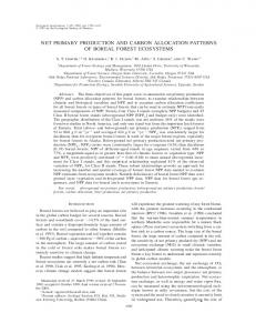
where T is an empirical constant which depends upon the values chosen for a and b. This approximation more clearly shows how nutrient mass transfer to coral reef communities directly depends on the non-dimensional quantities Cf, Sc, and Re* than the expression given in Eqn. 2.4. Mass transfer coefficients measured from the uptake of ammonium by experimental reef communities (Thomas and Atkinson 1997) are in very good agreement with the dissolution of gypsum-coated corals (Baird and Atkinson 1997) as described by the functional relationship given in Eqn. 2.11 (r2 = 0.95; Fig. 2.1). These results not only demonstrate that nutrient uptake by experimental reef communities occurs at the limits of mass transfer, but can be predicted from existing mass transfer relationships. If Eqn. 2.11 is dimensionalized, then the following relationship results: c

(2 . 12 )

Si

»

r

0 - * £ / 0 - 8 D 0 .5 8 £ 0 .2 v 0 .3 8

Dj for a specific dissolved nutrient and v can be calculated based upon the salinity and temperature of sea water (Li and Gregory 1974). Therefore, Eqn. 2.12 can be used to estimate the nutrient mass transfer coefficient (Si) once Cf, U, and k are known. From Eqn. 2.12 it also follows that Si is proportional to the benthic shear stress raised to the 0.4 power

14


(2.13)

St oc T°bA

This proportionality was corroborated by Hearn et al. (2001) who derived a similar expression based on a separate mass transfer relationship proposed by Batchelor (1967).

1.6

1.4 1.2

T

1.0

©

x 0.8

“ ca

(0

|

0.6

CO

0.4

v o * 0 +

0.2

0

0.5

1.0

1.5

2.0

2.5

gypsum HR rubble LR rubble p. compressa P.damicomis

3.0

3.5

R. a 5 ^ . 5 a (m S' 1 XU*4 ) °®k SCj Figure 2.1 Measured mass transfer coefficients for experimental reef communities based on ammonium fluxes (Thomas and Atkinson, 1997) and calcium fluxes (Baird and Atkinson, 1997) versus the quotient term in Eqn. 2.11. The model II regression shown is Y = 0.47X - 4e-6 (r2 = 0.95, n = 29).

15


Methods The purpose of this section is to show how Cf, U, and k across a Kaneohe Bay Barrier Reef flat community can be derived from measuring the height of waves propagating over the community. These values will be used to estimate the nutrient mass transfer coefficients for the community according to Eqn. 2.12.

Site description Kaneohe Bay is located on the northeast, or windward, side of the island of Oahu, Hawaii. The Kaneohe Bay Barrier Reef is roughly 2 km wide and 10 km long, running NW to SE along the entrance of Kaneohe Bay (Fig. 2.2). The only emergent structure on the Kaneohe Bay Barrier Reef is Kapapa Island. Most of the rest of the Kaneohe Bay Barrier Reef, including the reef flat and reef crest, remains submerged during all phases of the tide. The back-middle of the reef flat, however, becomes exposed only during very low tides. The depth of the reef flat ranges from < 1 m to ~3 m with a general trend in shoaling going from the reef crest to the back reef and from the Sampan and ship channels bounding each side of the reef to the middle of the reef flat. Despite the lack of emergent features, the presence of channels, and deeper portions of the reef flat, the Kaneohe Bay Barrier Reef is still very effective at dissipating the flux of wave energy incident to Kaneohe Bay. There are two primary sources of wave energy impinging on the Kaneohe Bay Barrier Reef: 1) wind waves 6-10 s in period generated by trade winds which blow out of the east to northeast all year round, but are most consistent during the

16


summer, and 2) ocean swells 10-14 s in period that originate from the north to northwest only during the winter months (Oct-Mar).

Kapapa Island

157°51.7’ Figure 2.2 Kaneohe Bay, Oahu, Hawaii. The Barrier Reef and patch reefs are outlined by the indicated 4-m isobaths. Wave characteristics were measured within a specific study area located towards the center and front of the reef flat (Fig. 2.3). This specific area was chosen on

17


hydrodynamic grounds for the following reasons. First, changes in wave heights appeared to be greatest in areas of the reef flat closer to the fore reef than near the back reef, providing the most robust estimates of changes in wave energy flux. Second, wave fronts moving across this area, and extending some hundreds of meters on either side of the area, were observed to be parallel and indicated only one predominant directional component (Fig. 2.4). Consequently, a 1-D linear array could adequately characterize losses in wave energy by monitoring changes in wave energy flux along a line in the direction of predominant wave propagation. Third, wave transformations within the study area should be dominated by dissipation due to bottom friction - the process which needs to quantified. The study area was also chosen based on its biogeochemical characteristics. First, it was an area in which estimates of net nutrient uptake, organic carbon metabolism, and benthic C:N:P ratios had already been made (Atkinson and Smith 1983; Atkinson 1987a; Chun-Smith 1994; Webb 1977, Atkinson, unpubl. data). This would allow me to place estimates of maximum nutrient uptake rates for this reef flat community in context with other observed biogeochemical characteristics taken from this area. Second, the substrate of the study area consists almost entirely of hard limestone populated mainly with groups of turf, macro-, and coralline algae with little sand. Therefore, it represents a nearly complete bioactive and autotrophic surface with few areas of minimal metabolic activity (Kinsey, 1985). The dominant genera of macroalgae within the study area include Sargassum, Turbinaria, Dictyota, Pedina, and Halimeda. The study area is also sparsely populated with fast growing heads of Pocillapora meandrina (0.1-0.3 m) as well as larger 18


heads of Porites lobata (0.5-1.5 m); however, corals represent a very small percentage of bottom type within the study area.

Figure 2 3 Instrument locations on the Kaneohe Bay Barrier Reef fla t Stations were ordinally numbered according to distance from the fore reef. Diamonds represent stations where both a current meter and a pressure sensor were deployed. Circles mark stations where only a pressure sensor was deployed. The dark color of the study area indicates nearly 100 % coverage of the benthos with algae and coral. Aerial image taken by AURORA and processed by E. Hochberg.

19


Figure 2.4 Same aerial image as shown in Fig. 2.3, but color-stretched to enhance the appearance of wave fronts. Select wave fronts are highlighted by yellow lines.

Wave height measurements Wave heights across the reef flat were measured on three different days corresponding to three different levels of incident wave activity during the summer of 2001 (10 Aug, 16 Aug, and 4 Sep). The dates used throughout this text represent the days on which the instruments were taken from the water. These measurements were made during the summer to ensure that the directional spectrum of waves incident to the 20


Kaneohe Bay Barrier Reef would have only one source: the trade winds. On each day four Seabird SBE-26 pressure sensors (Seabird Electronics, Bellevue, Washington) were deployed - 1 0 0 m apart in a linear array following the direction of predominant wave propagation with the first sensor located -50 m from the back of the surf zone (Fig. 2.3). The purpose for allowing space between the back of the breaking zone and the first station of the array was to allow broken waves to fully reform and to prevent the measurement of wave energy fluxes in an area prone to secondary breaking. In addition, the landward extent of the breaking zone can migrate in accordance with tidal changes in the depth of the reef flat. All pressure sensors were deployed on the bottom and programmed to sample at 2 Hz in fifteen minute-bursts every half hour, yielding 900 samples per burst. Each deployment lasted for approximately one day, yielding 40-43 wave bursts per deployment. The one-sided power spectral densities for wave height were calculated from the pressure sensor data using linear wave theory (Dean and Dalrymple, 1991). Each burst was treated as a single record and the resulting spectra from each burst was band-averaged by 10 fundamental frequencies into bands 1/90 Hz wide. Rms-wave heights, Hmu, were calculated for each burst from the total spectral energy during each burst (Horikawa 1988). Average significant wave heights (H»g) outside the Kaneohe Bay Barrier Reef were measured every half hour with a directional wave buoy (Datawell, Netherlands) deployed = 5 km off the Mokapu Peninsula, southeast of Kaneohe Bay (21°24.9’N, 157°40.7’W). H ^ is equal to y fl •

(Horikawa 1988).

21


Velocity measurements A MAVS-3 three dimensional current meter (NOBSKA, Mashpee, Massachusetts) was deployed ~1 m away from the pressure sensor closest to the fore reef on each of the three days (Fig. 2.3). The current meter was zero-calibrated in still water before each deployment and mounted in a free-standing, weighted tripod with its sensor positioned 0.S m off the bottom. Data from the u and v axes (i.e., the two horizontal axes) of the current meter were used to estimate the predominant direction of wave propagation by identifying the first principal component axis for each wave burst in u-v space.

Wave energy fluxes Waves propagating in shallow water develop a non-linear wave form (Dean and Dalrymple 1991). For shallow water waves, cnoidal wave theory provides the best description of wave dynamics and kinematics (Horikawa 1988). Isobe (1985) simplified the description of finite-amplitude waves in shallow water using first-order cnoidal wave theory. He gave the following expression for the wave energy flux, F (2.14)

F = f z P g H 24 g h

where p is the density of sea water, g is the gravitational acceleration constant, H is the wave height, and h is the depth of the water. The value of the constant iz depends on the degree to which the wave form is non-linear. The shape of the wave can be fully described by its associated cnoidal functions, however, Isobe (1985) created a simple

22


look-up table for the value of f2 based upon a wave-shape parameter called the shallow water Ursell number, Us, which is defined as (2.15) Us =

h

where T is the wave period. Higher values of Us represent increasingly non-linear wave forms. As Us approaches 1, the value of f2 approaches 0.125 and Eqn. 2.15 approaches the exact expression of F for shallow-water, linear waves. As Us gets larger, the value of f2 decreases continuously to a value of 0.0822 for Us equal to 200. This reflects the lower wave-energy density under an increasingly non-linear cnoidal wave form than would be predicted from linear wave theory (Horikawa 1988). F and Us were calculated for each burst using the rms-average wave height and peak spectral period. The rmswave height was chosen since it represented an average value of the wave energy density recorded over the length of each burst. The depth of the water, h, was determined by the mean bottom pressure during each burst.

Corrections fo r wave flu x divergence Increases in the flux of wave energy along the direction of wave propagation can occur due to the presence of energy sources such as wind stress and from convergence due to refraction. Decreases in the flux of wave energy along the direction of propagation can occur due to the presence of energy sinks such as breaking and bottom dissipation, and also from divergence due to refraction and diffraction. The area studied here was chosen to be well within the limits of the breaking zone so that wave breaking 23


would not be a factor in changing wave energy fluxes. Substantial changes in wave height and wave energy density occurred over tens to hundreds of meters. This is much too small a fetch for the predominant trade winds to add significant amounts of energy to surface waves propagating across the study area. Therefore, wind inputs were also neglected. There was some evidence of the divergence of wave fronts near the back side of Kapapa Island as well as over a slightly shallower part of the reef flat adjacent to the study area. This apparent loss can be estimated by conserving the total flux of energy along the length of an arc between adjacent wave-ray paths (Dean and Dalrymple 1991). Thus, the predicted wave energy flux at one point along the wave-ray path can be estimated from the wave-energy flux at a point upstream by their respective radii of curvature, Rj (2.16) where the subscripts i and i+1 represent adjacent stations. The expected change in wave energy flux owing to divergence would then be given as (2.17)

AFd

Changes in wave-energy fluxes due to bottom friction, AF6 , were then estimated from the observed differences in wave energy fluxes, A F , by subtracting the effects of wave divergence according to

24


(2.18)

AFbf

= AF -A F d

Even if the effects of bottom friction were neglected, then there would still be an apparent decrease in wave energy flux across the reef flat owing to wave energy flux divergence.

Estimating c / from rates o f frictional dissipation Because there was only one predominant direction of wave propagation within the study area, the spatial divergence in wave energy fluxes due to bottom friction could be reduced to a one dimensional problem (2.19)

V -F d/

dFbf = -JL

= - e bf

where r is a coordinate position along the direction of wave propagation and £b is defined to be a positive number. Eqn. 2.19 must also be made discrete because wave energy fluxes were estimated at discrete locations across the reef flat ( 2 .2 0 )

where (e*,) x denotes averaging with respect to distance. Furthermore, estimates of gradients in wave energy fluxes along the path of wave propagation needed to be corrected from observed differences in wave energy fluxes between adjacent stations according to (2.21)

Ar

= As cos a

where As is the distance between adjacent stations and a is the angle between the

25


direction of predominant wave propagation and direction of the line between adjacent stations. Estimates of F used here were time-averaged over an entire sample burst, thus they must be equated to rates of energy dissipation due to bottom friction which are also time-averaged over the burst interval (2 .2 2 )

= -fa )"

The rate of energy dissipation can be taken as the instantaneous product of the bottom shear stress with the near-bottom horizontal flow velocity, Uh, (2.23)

zbf

=

% -U k

where xb is the instantaneous shear stress vector at the bottom defined as (2.24)

%

= \ c f f>VkQk

where Uh = |c/A| . Eqn. 2.24 is the vector form of Eqn. 2.5. Substitution of Eqn. 2.24 into Eqn. 2.23 and time-averaging gives the following expression (2.25)

fa)'

= l C fp ( u l ) ' C os*

where $ is the average phase lag between the maximum bottom shear stress and the maximum bottom flow speed. For multi-spectral oscillatory flows, the use of a single phase-lag term in Eqn. 2.25 is a simplifying approximation. Eqn. 2.25 is analogous to an expression first proposed by Jonsson (1966) relating the average rate of energy

26


dissipation due to bottom friction to the maximum flow velocity in simple harmonic flow [Ub = Umsin(cot)] (2.26) where Umis the maximum flow speed. Jonsson (1966) defined fe based on energy dissipation in order to distinguish it from the friction factor used for estimating maximum bottom shear stresses (fw) based on the observed and predicted phase lag between bottom shear stress and velocity under sinusoidal flows (). It can easily be shown that if the phase lag, (j), is neglected, Cf = fe. For laminar flows, this phase lag is 45°. For turbulent flow over relatively small roughness elements this phase lag is only ~ 25° (Jonsson 1966; Jonsson 1980). Consequently, for rough, turbulent, sinusoidal flows, fe should be at least 90% the value of Cf. A review of the literature indicates that there should be little difference between fe and Cf for surfaces with faction coefficients in excess of 0 .0 S (Nielsen 1992). In the present chapter, I make no discrimination between Cf and fe and, therefore, choose to use Cf in order to be consistent with prior mass transfer and nutrient uptake literature. Averaging Eqn. 2.2S over space and replacing it in Eqn. 2.20 gives us an expression relating the difference in the time-averaged wave energy flux, the time- and space-averaged horizontal velocity cubed, and Cf

(2.27)

27


where the subscripts outside the brackets denote an average with respect to time and space, ( y t )

was calculated as the mean of ( y l'j

from each adjacent pair of

stations, which is equivalent to assuming that (y £ ) varied linearly between stations. By

plotting the left-hand term in Eqn. 2.27 versus i u \ ) we can use the model II ' /f.JC regression slope to get an average value of Cf for the reef flat community.

Results S

is dependent upon Uh, Cf, and k (Eqn. 2 .1 2 ). Thus, these parameters needed to

be estimated and/or measured from the characteristics of waves propagating across the reef flat.

Wave heights The mean significant heights of waves outside Kaneohe Bay during sampling were 1.9 m (10 Aug), 1.6 m (16 Aug), and 1.3 m (4 Sep). These values were lower than the mean daily significant wave height of 2.0 m over the two-year period between Aug 2000 and Jun 2002. Htms decreased 0.1S - 0.25 m across the reef flat from the most seaward to most landward stations (Table 2.1). Differences in Hmu across the reef flat between the three days varied according to differences in HSig outside Kaneohe Bay (Table 2.1). Mean wave spectral densities appear to be distributed in a broad, single peaked band from 0.05 to -0.35 Hz (Fig. 2.5-2.7). The absence of any significant energy 28


at frequencies greater than O.S Hz indicate that the data are not affected by aliasing. The peak in wave energy density for stations closest to the breaking zone occurred between 78

seconds in period on each of the three days corresponding to peak periods in the near

shore wave field. As expected, average wave heights were also substantially modulated with changes in tidal depth (Fig. 2.8, Table 2.1) owing to the shallow depth of the reef flat (1-2 m) relative to the tidal range (~0.6 m). This is because the maximum height of residual waves emerging from the break zone and propagating landward is primarily controlled by the depth of the water (Dean and Dalrymple 1991; Horikawa 1988).

10 Aug

16 Aug

4 Sep

Station

Mean

Range

Mean

Range

Mean

Range

I

0.40

0.35-0.45

0.30

0.20-0.38

0.23

0.18-0.27

2

0.27

0.23-0.31

0.24

0.14-0.32

0.19

0.13-0.24

3

0.18

0.14-0.22

0 .2 0

0.10-0.28

0 .1 2

0.07-0.17

4

0.16

0 . 12 -0 .2 0

0.13

0.05-0.21

0.09

0.05-0.14

Table 2.1 Mean and range in meters of rms-wave heights (Hnns) for each day at each station. The ranges are given by the minimum and maximum burst value from each deployment. Stations are ordered with increasing distance from the fore reef (Fig. 2.3).

29


£

0.8

0.8

0.6

0.6

0.4

0.4

0.2

0.2

CM

E 0

0.5

1

0.8

0.8

*5 0.6

0.6

0.4

0.4

0.2

0.2

©

Q

5 © Q. CO

0

0.5

1

0

0.5

1

0

0.5

1

Frequency (Hz) Figure 2.5 Power spectral densities of surface wave height for each of the four stations on 10 Aug 2001. Mean spectra are given by the thick black line. The gray regions represent the 95% confidence interval for the mean spectra. The dashed lines represent one standard deviation for all spectra. Stations are ordered with increasing distance from the fore reef.

30


0.5

0.5

0.4

0.4

0.3

0.3

*7 N X

no

0.2

‘g

0.1

0.1

IT § 9

0

0.5

1

0.5

0.5

0.5

0.4

0.4

0.3

0.3

0.2

0.2

0.1

0.1

S 8

Q. 05

0.5

0

0.5

Frequency (Hz) Figure 2.6 Power spectral densities of surface wave height for each of the four stations on 16 Aug 2001. Mean spectra are given by the thick black line. The gray regions represent the 95% confidence interval for the mean spectra. The dashed lines represent one standard deviation for all spectra. Stations are ordered with increasing distance from the fore reef.

31


1

Tn X

0.25

0.25

0.20

0.20

0.15

0.15

0.10

0.10

0.05

0.05 0

0.20

«

0.15

0.15

0.10

0.10

0.05

0.05

2

0

0.5

1

0

0.5

1

0

0.5

1

Frequency (Hz) Figure 2.7 Power spectral densities of surface wave height for each of the four stations on 4 Sep 2001. Mean spectra are given by the thick black line. The gray regions represent the 95% confidence interval for the mean spectra. The dashed lines represent one standard deviation for all spectra. Stations are ordered with increasing distance from the fore reef.

32


0.5

2.0

10 Aug AS _

1.8

0.4 1.6

r2 = 0.21 15:00

18:00 21:00

00:00 03:00 06:00

09:00

0.5

1.4 2.5

16 Aug

0.4

2.0

E CO

\

X 0.2 0.1

1.5

r2 = 0.90 12:00

15:00

18:00 21:00 00:00 03:00

06:00

0.3

1.0

2.5

4 S ep 0.2

2.0

r2 = 0.90 0.1

15:00

18:00 21:00 00:00 03:00 06:00

09:00

1.5

Time Figure 2.8 Depth (dashed line) and rms-wave height (solid line) at stations closest to the fore reef on 10 Aug, 16 Aug, and 4 Sep 2001 versus time, along with the correlation between each pair of time-series. Note the similarity in the shape of each 10 Aug time-series despite the poor correlation. 33


Tidal depth (m)

0.3

Wave-driven velocities Spectral densities of horizontal wave-induced, horizontal flow velocities were calculated from the current meter data by adding spectra calculated from the u and v axes. The resulting spectra were similar in shape and magnitude to those predicted by linear transformation of the pressure sensor data (Dean and Dalrymple 1991; Fig. 2.9). However, spectral densities calculated from the current meter data were significantly lower than those derived from the pressure sensor data, especially for the highest spectral densities and for the more energetic days. Based on data and estimates of the friction coefficient presented here, horizontal flow speeds should be >99% their potential flow values at a distance of -0.5 m from the bottom (Hearn 2001; Nielsen 1992). Isobe (1983) showed that observed orbital velocities under shallow-water waves propagating over a gently sloping bottom were lower than those predicted from wave theory. The data presented here indicate that the correction for shallow-water wave orbital velocities predicted from wave heights using linear theory depends primarily on the magnitude of the spectral density and not on its frequency (Fig. 2.10), suggestive of a missing non linear correction. Results from all three days yielded similar deviations from prediction based on linear wave theory despite data from each day showing a different range in spectral densities. Using the empirical correction to the linear transfer function shown in Fig 2.10, near-bottom horizontal velocities were predicted from the pressure sensor data. Time-averaged, near-bottom horizontal flow speeds varied between 0.081 and 0.214 m s '1; decreasing with increasing distance from the fore reef and with decreasing H,jg outside Kaneohe Bay (Table 2.2). 34


0.8

10 Aug

0.6 0.4 0.2

0 Tn X CM

co

0.1

0.2

0.3

0.4

0.5

0.6

0.7

0.8

0.9

1

0-4 r

16 A ug .

0.3 -

CM

E

~

0 .2

-

CO

§ Q

0.1 -

0

0.1

0.2

0.3

0.4

0.5

0.6

0.7

0.8

0.9

1

0.2

4 Sep 0.1

0

0.1

0.2

0.3

0.4

0.5

0.6

0.7

0.8

0.9

1

Frequency (Hz) Figure 2 3 Mean power spectral densities of near-bottom horizontal velocities for 10 Aug, 16 Aug, and 4 Sep 2001 as measured directly with a 3D current meter (solid line) and predicted from pressure sensor measurements using linear transformations (dashed line). 35


1.2 1.0 . a = 0.71

b = 0.91 0.8 - r2 = 0.98 0.6 . N = 3560 0.4

10 A ug

0.2 0.2

£ %>

> 3 '35 c Q

12 1.0 .

8.

0.6

1

0.8

T

1.0

1.2

T

a = 0.72 b = 0.94 0.8 ‘ r2 = 0.99 0.6 . N = 3827 0.4

16 A ug

0.2

2 CO

0.4

1o

0.2

0.4

0.6

0.8

1.0

1.2

1.2

a = 0.74 b = 0.91 r2 = 0.98 N = 3870

1.0 0.8 0.6

0.4

4 S ep

0.2 0

0.2

0.4

0.6

0.8

1.0

1.2

Spectral Density [P] (m2 S'2 Hz-1) Figure 2.10 Power spectral densities for all frequencies from all bursts for 10 Aug, 16 Aug, and 4 Sep 2001 as calculated from the current meter data [uv] and predicted from the pressure data by linear transformation [P]. The dashed lines represents a 1:1 relationship. The solid lines represent a least-squares regression of the form Y = aXb. For data pooled from all three days, a = 0.71 and b = 0.91 (r2 = 0.98, N = 11,257).

36


4 Aug

16 Aug

4 Sep

Station

Mean

Range

Mean

Range

Mean

Range

1

0.214

0.191-0.233

0.164

0.133-0.185

0.116

0.100-0.131

2

0.167

0.147-0.188

0.148

0.104-0.179

0.119

0.099-0.136

3

0.126

0.107-0.126

0.137

0.092-0.162

0.086

0.062-0.112

4

0.119

0.098-0.139

0 .1 0 2

0.058-0.132

0.081

0.057-0.104

Table 2.2 Mean and range (m s*1) o f time-averaged, near-bottom horizontal flow speeds (u h^ for each day at each station. The ranges are given by the minimum and maximum burst value from each deployment. Stations are ordered with increasing distance from the fore reef (Fig. 2.3). Cross-reef currents Mean cross-reef currents, calculated as the mean horizontal velocity over each 15minute burst, were typically less than 0.02 m s' 1 for each of the three deployments (Fig. 2.1 1). Consequently, wave-current interactions were not considered in the treatment of wave transformations and bottom friction.

Wave energy flu x divergence The predominant direction of wave propagation (and wave energy flux) was nearly constant throughout each deployment (Fig. 2.12). Greater than 93% of the wave energy flux occurred along one axis on all three days. The direction of predominant wave propagation diverged -15° over an arc-distance of -150 m at the most seaward stations of the reef flat (Fig. 2.12). This would indicate a radius of curvature of -570 m 37


0.04 0.03 0.02 0.01 -

-

10 A ug

0.01 0.02 15:00

18:00

21:00

00:00

03:00

06:00

09:00

E 2

0.04 0.03

3

0.02

' 0 ■O

218

X 3

214

18:00

21:00

00:00

03:00

06:00

09:00

216

212

>

I

15:00

220

.o o S

0

10 A ug

mean = 225'

210

16 A ug

mean = 217' 12:00

15:00

18:00

21:00

00:00

03:00

06:00

215 213 211

209 207 205

4 S ep

mean = 210' 15:00

18:00

21:00

00:00

03:00

06:00

09:00

Figure 2.12 Principal direction of wave propagation determined from the current meter on 10 Aug, 16 Aug, 4 Sep 2001. The principal axis carried >93% of the variance in flow speed on all three days.

39


in the shape of the propagating wave fronts. This is consistent with visual interpretation of propagating wave fronts from an aerial photograph of the Kaneohe Bay Barrier Reef which indicate a radius of curvature of -7(30 m near the most seaward stations and decreasing towards the back of the reef flat (Fig. 2.4). Based on the above considerations, R at the most seaward stations was taken to be equal to 630 m. Although this method of estimating wave-energy flux divergence is simplistic, the data presented here indicate that this process typically contributed at most 20-30% of the observed f

decline in wave-energy fluxes across the study area

A 17

\

AF

Estimation ofc/ Since flow measurements were made only at the most seaward station of each array, the time-averaged horizontal flow speed cubed, ( ^ a) » was estimated from the pressure sensor data using an empirical correction to the linear transfer function as described earlier. There was generally very good agreement between estimated values of ( y l ) 311(1 those calculated directly from the current meter data (Fig. 2.13). Results from regression of Eqn. 2.27 yielded a value of Cf equal to 0.22 ±0.02 (p < 0.025, r 2 = 0.91, n = 338) for the study area of the reef flat (Fig. 2.14). Changes in the wave energy flux between the last two stations of the array on Aug 10 were not included in the regression since they appear to cluster away from the other data lying near the regression 40


r2 = 0.99 n = 126

0.04

•% co

0.03

7

3 V

0.01

0

0.01

0.02

0.03

0.04

t [uv] (m3 s '3) Figure 2.13 Time-averaged near-bottom horizontal flow speeds cubed as predicted and corrected from sensor data [P] and as directly computed from current meter data [uv]. The solid line represents a 1:1 relationship. line. This is likely due to non-local inputs of wave energy from the area of the Kaneohe Bay Barrier Reef northwest of Kapapa Island on this most energetic day. The northwest half of the reef flat is deeper (2-3 m) than areas of the reef flat southeast of Kapapa Island and could have allowed for the transmission of wave energy to the most landward station 41


where observed wave energy densities would be higher than expected. Separation of the data from all three days into three pairs of stations with increasing distance from the fore r a f indicated that Cf did not vary significantly with distance across the study area (p < 0.025). Uncertainty in the estimate of Cf for the reef flat community can also come from uncertainty in the radii of curvature for the diverging wave fronts (Eqns. 2.17 & 2.18). However, an uncertainty of ± 200 m in the radii of curvature estimated here translates into an equivalent uncertainty of only ± 5% in the value of Cf, or ± 0.01. Consequently, the uncertainty in Cf is ± 0.03 or ± 14%.

Estimation o f k based on c/ Estimates of k based on Cf can be obtained from the literature on turbulent, oscillatory flow over rough surfaces. Reef communities are typically heterogeneous surfaces lacking a singular roughness scale. For this reason, the roughness height, k, was derived from estimates of Cf. Flow conditions across the study area met the criteria for rough, turbulent, oscillatory (Kamphuis 1975) based on the estimated friction factors and relevant Reynolds numbers. Nielsen (1992) reanalyzed various experimental data on the friction generated by oscillatory flow over rough surfaces (Jensen 1989; Kemp and Simons 1983; Riedel 1972; Sleath 1987; Swart 1974) and gave the following empirical expression = exp 5.5

f L-')0.2

-6 3

42


7

6

Cf= 0.22 ± 0 .0 2 r2 = 0.91

5 m co

4

UCL

ao

3

CM

2

1

0 0

0.01

0.02

«

xK

0.03

s ' 3)

Figure 2.14 Values for the left-hand term in Eqn. 2.27 (see text) versus (UhJ between all stations on all days (circles) except from between stations #3 and #4 on 10 Aug (dots, see text). Model II regression gives the equation Y = 0.22X 0.0003 (N - 338), where the value of the slope gives the best estimate of Cf.

43


where k is the roughness height as described before, A is the horizontal orbital excursion amplitude, and fwis the friction factor relating the maximum shear stress to Um2. For simple harmonic flows, the exact relationship between fwand fe (Kajiura 1968) is (2.29)

3zrcos0

where the ratio in parentheses is « 1, given a value of 0 ~ 25° cited earlier. Furthermore, the literature review by Nielsen (1992) revealed that fw= fc for turbulent, oscillatory flow over rough bottoms within the variability of experimental data. For the present purposes I will thus consider that Cf = fw= fe. Kamphuis (1975) also gave an expression to obtain fwfor the conditions of A/k < 100 which apply here (2.30) Based on the data presented here, fw as estimated by Eqn. 2.30 should also be between 0.10 and 0.40. Nelson (1996) used a relationship similar to that of Eqn. 2.28 (Swart 1974) to estimate the average roughness height of a shallow reef from values of fe. For the data presented here, the rms-orbital amplitude, Anns, varied from 0.2 m at the most back-reef stations to 0.6 m at the most fore-reef stations. Using the value of Cf estimated before and a mean Anns of 0.4 m for the study area, we get an average k for the study area of 0.20 m from Eqn. 2.28 and 0.18 m from Eqn. 2.30. Based on these results, a value of 0.2 m was chosen to represent the roughness height of this reef flat community. This values is consistent with observations of roughness height made in the field. 44


Estimates o f nutrient mass transfer coefficients S was calculated based on the regression shown in Fig. 2.1. This assumes that the mass transfer relationship is the same under steady and oscillatory flow. Mean values for the nutrient mass transfer coefficient, Si, across the study area were estimated for each station over the entire duration of each deployment (Table 2.3). The relationship in Eqn. 2.12 assumes that S is proportional to Uh0'8, therefore, the time-averaged values of Uh0'8 were used to estimate mean values for S. Estimates of S for phosphate, Sp, ranged between 3.6 and 7.1 m day'1 while values of S for both ammonium and nitrate, Sn, varied between 5.9 and 12.0 m day'1. By Eqn. 2.12, the reported uncertainty in Cf would translate into an uncertainty in S of only about ± 5%. Uncertainty in estimates of S resulting from the regression shown in Fig. 2.1, based on 95% confidence limits, are about ± 0.5 m day'1for dissolved phosphate and ± 0.7 m day*1 for ammonium and nitrate. Given that mean significant wave heights outside the bay were 2.0 m over a two-year period, I will consider the conditions on 10 Aug to be representative of average nutrient mass transfer coefficients for that particular reef flat community. Using a mean (Uh)t over all stations from this day alone gives an average Sp equal to 5.8 ± 0.8 m day'1 and Sn equal to 9.7 ± 1.3 m day'1.

45


(A) Dissolved phosphate Station Date

1

2

3

4

10 Aug

7.1

6.0

4.9

4.7

16 Aug

5.8

5.4

5.2

4.2

4 Sep

4.5

4.7

3.7

3.6

(B) N itrate and ammonium Station Date

1

2

3

4

10 Aug

12.0

10.0

8.1

7.8

16 Aug

9.8

9.1

8.6

6.9

4 Sep

7.6

7.8

6.2

5.9

Table 2.3 Estimates of maximum nutrient mass transfer coefficients for (A) dissolved phosphate, and (B) both nitrate and ammonium in m day'1for the Kaneohe Bay Barrier Reef flat. The diffusivity of dissolved phosphate was calculated as the weighted average of the diffusivities of dissolved phosphate species based upon their relative abundance in sea water (Li and Gregory 1974; Morel 1983). Values for species diffusivity and v were estimated based on measured temperatures and a salinity of 35 psu. The roughness height, k, was assumed to be 0.2 m (see text for details).

Discussion Comparison o f Cf results with other reefs The friction coefficient reported here for the Kaneohe Bay Barrier Reef flat (C f= 0.22 ± 0.02) is comparable with values for the friction coefficient estimated for other reefs such as Ala Moana Reef, Hawaii (fe = 0.28 ± 0.25; Gerritsen, 1981) and John

46


Brewer Reef, Great Barrier Reef (fe = 0.15 ± 0.04; Nelson, 1996). Each of these average values is close to the proposed asymptotic limits for the value of fe (0.25-0.30) mentioned earlier. Estimates of k derived from Eqns. 2.28 & 2.30 are similar to visual estimates made in the field and correspond to values of A/k ~ 2. Kajiura (1968) proposed a theoretical limit of fw= 0.25 for A/k < 1.67. However, in reviewing a greater number of experimental data sets, Jonsson (1980) indicated that a constant value of fw= 0.30 should be used for A/k < 1.57. Both of these results can explain why the estimate of Cf reported here is close to this asymptotic limit; i.e., of order 0.1 as opposed to order 0.01. It can also explain why Cf did not vary significantly across the study area (p < 0.025). The comparably high values of fe or Cf for different reefs may result from the magnitude of their roughness heights being of similar scale to wave orbital excursion amplitudes. More data will need to be collected before generalizations on the high frictional roughness of reef communities under waves can be made.

Past estimates o fS Bilger and Atkinson (1992) underestimated Cf for the same Kaneohe Bay Barrier Reef flat community a factor of 10-20 lower as compared with the present estimate of Cf. This discrepancy translates into estimates of St and S that are a factor of 2.5-3.3 lower than estimated here. In a paper contemporary with Bilger and Atkinson (1992), Atkinson (1992) estimated the rate of phosphate uptake for two windward Enewetak Atoll reef flats based on mass transfer correlations using a value of Cf which was a factor of 10-20 times lower than that of the Kaneohe Bay Barrier Reef flat and other reefs (Gerritsen 1981; 47


Nelson 1996). The much greater ability for coral reef communities to transfer momentum (i.e., higher friction coefficients) than previously known by coral reef biogeochemists implies a greater ability to transfer mass. Bilger and Atkinson (1992) did not have any measurements of flow velocities across the Kaneohe Bay Barrier Reef flat available to them and used an average velocity of 0.06 m s'1in their calculations based on prior estimates of cross-reef transports (Atkinson 1987a; Bathen 1968). This is much lower than typical horizontal flow speeds measured here. The authors estimated average flow speeds induced by the passage of a 0.5-m solitary wave and estimated a value of 0.19 m s '1, however, they only suggested that “wave surge” may be an important source of mass transfer enhancement. Furthermore, it is clear that flow velocities across the Kaneohe Bay Barrier Reef flat cannot be characterized by a single velocity scale derived from a single wave form. Atkinson (1992) had unpublished velocity and depth data for his calculations, but did not report any information regarding the spatial and temporal variability in these measurements, nor how they were collected.

Variations in S driven by wave transformation Changes in Cf across the study area were not significant (p < 0.025). Furthermore, S depends on Cf only to the 0.4 power (Eqn. 2.12). Therefore, spatial and temporal variation in S across the study area should result primarily from variations in horizontal flow speed (U h, Eqn. 2.12, Table 2.2). Spatial variations in Uh across the reef flat are driven by attenuation of residual waves moving out of the surf zone (Table 2.1 & 2.2).

48


Because most reef flats lie behind a breaking zone, the wave environment over most reef flats will be influenced by the wave breaking process. In the simplest description of depth-induced breaking, waves of a given height break when they exceed some fraction (y) of the water depth, h (Dean and Dalrymple 1991; Horikawa 1988) (2.31)

# max = Yh

The effect of depth-induced breaking is similar to that of an amplitude filter, reducing the height of waves which exceed the maximum allowable height. Wave breaking was observed to occur continuously on all three days, yet H rds and Uh varied between days according to the mean significant wave height outside Kaneohe Bay (Tables 2.1 & 2.2). This indicates that the average height of residual waves propagating from the surf zone are still influenced by the height of waves outside the breaking zone despite the amplitude-filtering effects of depth-induced breaking. Therefore, temporal variations in S across the reef flat are still influenced by variation in wave heights outside Kaneohe Bay, albeit substantially damped by the wave breaking process. The height c f residual waves propagating from the surf zone can also be modulated by tidal changes in water depth (Fig. 2.8, Table 2.1). Such tidal regulation of wave transformation and attenuation near coral reefs has been documented elsewhere (Lugo-Fernandez et al. 1998a, 1998b). Tidally induced variations in Hnm across the reef flat were relatively greater than variations in Uh (Tables 2.1 & 2.2). This is because shallow-water wave-orbital velocities are proportional to wave height, but inversely proportional to the square root of the water depth according to linear approximation

49


{U h °c h /•sfh ; Dean and Dalrymple, 1991). Thus, increases in Uh that follow increases in Hrms on a rising tide are partially offset by the increasing kinetic energy of the larger waves being distributed over a deeper water column. Near-bottom horizontal flow speeds were significantly and positively correlated with depth for all stations (p < 0.01) except for stations 1 and 2 on 10 Aug (Table 2.4). The lack of a positive correlation for these stations on 10 Aug is likely due to differences in amplitude modulation for the two time-series. Changes in mean flow speeds for these two stations still appeared to be driven by the tide (data not shown), much like the case for Hnns (Fig. 2.8).

Station

r2 10 Aug

r2 16 Aug

i^4 Sep

1

ns

0.64

0.71

2

ns

0.67

0.81

3

0.38

0.76

0.95

4

0.73

0.89

0.95

Table 2.4 Correlation coefficients between tidally induced changes in depth and mean near-bottom horizontal flow speeds. Values for r2 which were not significant for p < 0.025 and are designated by ‘n s \

50


I ll

NUTRIENT MASS TRANSFER RATES DERIVED FROM THE DISSOLUTION OF PLASTER MOLDS

Introduction Chapter goals The first goal of this chapter is to use the dissolution of plaster molds to provide estimates of nutrient mass transfer coefficients for a Kaneohe Bay Barrier Reef flat community. The second goal of the chapter is to examine the importance of different roughness scales relevant to coral reef communities (0.001 - 0.1 m) on rates of nutrient mass transfer for a given surface. The third goal is to determine whether there is a significant difference between rates of nutrient mass transfer under the steady flow conditions of an experimental flume used in prior mass transfer experiments with the in situ, wave-driven flows to which natural reef communities are exposed.

Background: The utility o f dissolving plaster surfaces The dissolution of plaster, or gypsum (CaSCV2H20), is widely used in aquatic sciences to characterize water motion because plaster forms have been shown to dissolve faster at higher flow speeds (Muus 1968; Doty 1971; Thompson and Glenn 1994;

51


Santschi et al. 1991; Jokiel and Morrisey 1993; Porter et al. 2000). These observations can be explained by mass transfer theory. Baird and Atkinson (1997) showed that mass transfer correlations could accurately predict rates of dissolution of gypsum-coated corals in experimental communities once the flow velocity and frictional characteristics of the community were known. In an earlier work, Thomas and Atkinson (1997) showed that mass transfer correlations could accurately predict rates of ammonium uptake by experimental communities of coral and turf-covered coral rubble which varied in relief and frictional roughness. The agreement between these two studies demonstrated how the dissolution of plaster surfaces could be used to describe the mass transfer of nutrients. This is because the diffusivities of the major ions in gypsum (Ca2+ and SO42') and dissolved inorganic nutrient species (e.g., PO43', H PO 42*, N lV , and N 0 3‘) are of the same scale (Li and Gregory 1974).

Methods The basic approach was to 1) fabricate plaster (gypsum) surfaces of varying morphological character, 2) deploy these molds under different flow conditions, 3) estimate the rate of mass transfer from the mold by measuring changes in the weight of the plaster mold before and after a deployment, and 4) compare these rates with mold surface areas.

52


Plaster mold design Plaster molds were constructed using rectangular plaster forms, or elements, of square cross-sectional area (6.1 x6.1 cm2). Anywhere from 8 to 22 of these forms, 4-15 cm in height, were placed upright on a tray made from 0.32 cm-thick sheet aluminum. The sides of the tray were -2-2.5 cm high and were easily formed by bending the aluminum sheet in a vise to form right angles. The purpose of these sides were three fold: 1) to give the light aluminum tray more strength, 2) to provide a reservoir into which additional plaster could be poured, thus creating a surface entirely made of plaster, and 3) to help secure the individual elements in place and reduce the fragility of the entire mold. Two sizes of square aluminum trays were used throughout this study: one set 0.5x0.5 m and another set 0.38x0.38 m. The reason for the change in tray size was to create molds that could be deployed inside a re-circulating flume as well as in the field. Three threaded, stainless steel rods (lOx 1.3 cm) were used as bolts to hold two anchor bars to the bottom of the tray (Fig. 3.1 A). The anchors were made from 1x 10 cm mild steel bar. The threaded rods extended ~5 cm below the anchors, forming legs for the plaster mold. The extension of the bolts allowed the mold and anchors to sit above any roughness < 5 cm in the field. PVC irrigation pipe 2 3 cm in diameter dammed each bolt hole from plaster being poured into the tray and were sealed to the tray with silicone. Plaster elements and molds were prepared using US Gypsum (Chicago, Illinois, USA) No. 1 pottery plaster (% by weight: 96.2% {3-hemihydrate [CaSCV I/ 2 H 2O], 0.5% CaS04, 2.4% dolomite [CaMg(C0 3 )2], 0.4% oxides, 0.5% acid insolubles). This composition was checked against an analysis of the material by inductively coupled 53


plaster elem ents

b a s e plate

rods anchor bars

B

d

< 3

d d

d d

d

d d

d

d

Figure 3.1 (A) Top-view schematic of smaller mold design. (B) examples of elements with different roughness scales.

54


plasma and optical emission spectroscopy (Baird and Atkinson 1997). The plaster powder was hydrated using tap water to form solid gypsum by the following reaction (3.1)

CaSOi / 2H 20

+

y2H 20

->

CaS04 2H z0

The plaster powder was mixed in a 5:4 vohvol ratio for 1.5 minutes before being poured into 6 x 6 x 100 cm flexible PVC molds. Care was necessary to ensure that the mixture remained as inviscid as possible in order to prevent the formation of bubbles during casting. After the plaster was allowed to fully set, individual elements were cut from these solid plaster bars. Plaster elements were then placed in an evenly distributed and staggered array on the aluminum tray (Fig. 3. IB). Finally, a wet plaster mixture of the same composition was poured into the tray until the meniscus of the liquid plaster was just above the rim of the aluminum tray. This pouring was done to secure the elements in place as well as to create a continuous plaster surface. It was necessary to soak the plaster elements for a few minutes before the second pouring in order to prevent the dry elements from absorbing too much water from the wet plaster. Large cracks would form in the base layer of the molds if this precautionary step was not followed. Plaster molds were soaked for four hours in seawater before deployment and weighed 30-60 minutes after being removed from the water. A period of four hours was determined to be adequate after a larger-than-average dry plaster element ( 1 0 x 1 0 x 20 cm) was soaked in water for four hours, cut in half, and shown to be saturated to its core. The molds were left to stand 30-60 minutes before initial weighing to recreate the similar amount of time required to pick up the molds from the field and bring them back to the 55


Hawaii Institute of Marine Biology by boat. Each mold weighed between 8-20 kg, with typical weight losses over a deployment varying between 0.5 and 2 kg, or -5-10% of the wet weight of the molds. To convert weight loss of wet plaster to loss of calcium in moles, an experiment was performed to determine the ratio between the densities of dry and wet plaster (Pdry/Pwet)- Three batches of plaster were separately prepared in the same way as for the molds. The liquid plaster from each batch was poured into two 0.5-L plastic cups approximately 8 cm in diameter and 12 cm high and allowed to sit overnight. The following day all six solid plaster forms were soaked in water for four hours, allowed to sit for 30 minutes, and then weighed before being placed in a temperature-controlled oven at 55°C. The forms were then weighed four times over the following four days after which Pdry/Pwet had reached an equilibrium value of 0.64 ± 0.02 (Fig. 3.2). The weight of plaster lost from a mold over the duration of a deployment (AWwet) could then be converted into the mass of calcium lost (AMca) by the following equation (3.2)

AM r. =

fj^SL

where MWgyp is the molecular weight of gypsum (172.1 g).

56


o batch 1 v batch 2 □ batch 3

o> '53 JS co c

0

20

40

60

80

100

120

140

Time (hours) Figure 3.2 Change in density of plaster elements with time following drying in an oven at 55°C.

Mass transfer o f Co1* from dissolving gypsum surfaces The simplest mass transfer formulation relates the flux of a species, Ji, from a surface to the difference between the concentration of that species in the ambient fluid, Q .b ,

and adjacent to the surface, Q . w, by the mass transfer coefficient, S i

57


(3.3) The mass transfer coefficient can be expressed as the product of the nondimensional Stanton number, St, and the ambient flow speed, U (3.4)

S{ = Stt U

Rates of mass transfer for dissolved major ions such as Ca2+ and SO42', as well as dissolved nutrients (e.g., NH4+, NO3', HPO42*), are characterized by high Schmidt numbers (500-1500). The Schmidt number (Sc) is a non-dimensional quantity defined as the ratio of the kinematic viscosity of seawater to the diffusivity of the ion in question (Sc = v/Di). The dependency of Si and Stj on Sc for high Sc (< 4600) is (3.5) (Dawson and Trass 1972). Because Sc is dependent on temperature, all mass transfer estimates were normalized to a temperature of 25°C. Eqn. 3.5 indicates that Si should be a function of the species diffusivity, D i, raised to the 0.58 power. Consequently, the ratio of mass transfer rates for two species, A and B, in the same fluid can be described by the following proportionality

The dissolution of gypsum involves the liberation of free Ca2+ and S0 4 2‘ ions in equal proportions (3.7)

CaSOx -2HzO => Ca2+ + SO ? + 2H 20

58


Therefore, the flux of total Ca2+ and total S 0 42' (ZCa2+ and ZSO42’, respectively) must be equal to satisfy both charge and mass balance: (3.8)

JZCa = J zso.

The solubility products of gypsum in sea water of varying salinity and temperature have been calculated using Pitzer-type ion-interaction models (Krumgalz and Millero 1983; Thompson and Glenn 1994). Results from these calculations have been in very good agreement with direct measurements (Culberson et al. 1978). In these ioninteraction models, solubility products are calculated from total ion concentrations and total ion activity coefficients. The total concentration of an ion is equal to the concentration of the free ion plus the concentrations of all the ion pairs that it forms. Significant fractions of both Ca2+ and SO42' form ion pairs with other major ions in seawater (Stumm and Morgan 1981). Therefore, the mass transfer coefficient of each of these ion-pairs will differ according to their own specific diffusivity, as estimated by the following equation (Lide 2000) (3.9)

z+ D:++|z_|ZV

The diffusivities of flee Ca2+ and S 0 42‘ in seawater at 25°C, 35 psu, and 1 atm are 7.5xlO*10 and 9.8xl0‘l° m2s'1, respectively (Li and Gregory 1974). If characteristic diffusivities for ZCa2+ and Z S042' are calculated using a weighted average of the diffusivities of the free ions and their ion pairs based upon their relative abundance in seawater (Pytkowicz and Hawley 1974), the average diffusivities of ZCa2+ and ZS0 4 2*are

59


7.6xlO'10 and 10.3xl0'l° mV1, respectively, not much different from that of their free ions. Furthermore, the diffusivities of all ion-pairs differ from the diffusivities o f free Ca2+ and free S 0 42" by only 10-20%. This would imply that the individual mass transfer coefficients for each of the ion pairs would differ by only 5-10% from that of free Ca2+ and free S 0 42*(Eqn. 3.8). Furthermore, the elevation of ZCa2+ and Z S042' concentrations near the wall of the gypsum surface would imply that the relative abundance of the free ions should increase relative to standard seawater. Consequently, an even greater proportion of ZCa2+ and Z S042’ mass transfer will be carried by their free ions than indicated by their relative abundance in standard seawater. Therefore, the diffusivities of ZCa2+ and XS042' (from herein represented simply as Ca2+ and S 0 42 ) were calculated using the weighted diffusivities of both free ions and ion pairs, with small corrections for temperature as directed by Li and Gregory (1974). Using Eqns. 3.3 and 3.8, we can define the following mass balance equation

(3.10)

Sc.([Ca” l- |< V * L ) _ ^ S a O s O j - l - b o r U

where 0^* according to Eqn. 3.6. The concentrations of Ca2+ and S 0 42*at the wall are given by the following solubility product for gypsum (3.11)

[C 1-2 cm s*1 over the course of an individual dissolution experiment (Table 3.1). Water temperatures across all field and flume experiments ranged between 23°C and 27°C, leading to temperature-dependent corrections of » (0

■o

(0

y

o

20

E

•a. 0

0.2

0.6

0.4

0.8

1.0

Surface A rea (m2) Figure 3.9 Rate of calcium loss for all molds versus surface area for all field experiments. The open symbols represent molds while the closed symbols represent individual elements projected to be entire molds. All rates were normalized to a temperature of 25°C. 76


1.2

10

flat 8

smooth holes grooves

0.206 0.179 0.143 0.061 0.021

m s' m s' m s' ms ms

6 >* T3 (0

E, co

4

2

0

a Figure 3.10 Calcium mass transfer coefficient versus the ratio of surface to projected area (a) for all Held experiments. The open symbols represent molds while the closed symbols represent individual elements projected as entire molds. All rates were normalized to a temperature of 2S°C. The dashed line represents the minimum allowable value for a.

77


6

5

* □ O V

flat smooth holes grooves

4 >* T3 CO

E,

3

co 2

1

0

1

2

3

4

a Figure 3.11 Calcium mass transfer coefficient for all molds versus the ratio of total surface area to projected area (a) for flume experiments. The open symbols represent molds while the closed symbols represent individual elements projected as entire molds. All rates were normalized to a temperature of 2S°C. The dashed line represents the minimum allowable value for c l

78


Flume vs. Field experiments The Stanton number, St, describes the rate o f mass transfer a given surface will support at a given flow speed. Therefore, in order to compare results from molds of different surface area within an experiment, St needs to be normalized by a . As expected mean St/a decreased with (Uh){ for all field experiments (Fig. 3.12). This relationship is consistent with results from past flume experiments (Baird and Atkinson, 1997; Thomas and Atkinson, 1997; Fig. 3.13). Mean S t/a for the flume experiments was significantly lower (p 0.1. Consequently, changes in Jpmax and N P P across the reef flat are driven by both changes in Uh and phosphate concentration. (Uh)t in the back half of the reef should be typically

Nutrient uptake and net primary production

Nutrient uptake and net primary production

Suggest Documents

Nutrient uptake and primary productivity in an urban estuary: using

Nutrient uptake, nutrient availability and quality ...

Fluoride Uptake and Net Primary Productivity of Selected Crops

Biomass Production, Nutrient Uptake and Partitioning in ... - CiteSeerX

Studies on dry matter production, nutrient uptake and ... - Google Sites

Assessment of forest net primary production

Net primary production of terrestrial ecosystems

COMPONENTS OF NET AERIAL PRIMARY PRODUCTION ... - SciELO

MEASURING NET PRIMARY PRODUCTION IN FORESTS ...

Measuring Net Primary Production in Forests

Net Primary Production in the Shortgrass Steppe

Assessing Net Primary Production in Montane ...

Benthic and planktonic primary production along a nutrient gradient in ...

Excess primary production, calcification and nutrient ... - Inter Research

Patterns of primary production and nutrient availability in a ... - FAU

Primary production and nitrate uptake within the seasonal thermocline ...

Net primary production and carbon stocks in ... - Dimitrios Gyalistras

Effect of precipitation variability on net primary production and soil ...

Gross and net primary production: closing the gap ... - Inter Research

Net primary production and soil respiration in New ... - Harvard Forest

and Belowground Net Primary Production in a Temperate Mixed ...

Net primary production and carbon cycling in coast ...

net primary production and carbon allocation patterns of boreal forest ...

Interannual Variability in Net Primary Production and Precipitation