O(1) Delta Component Computation Technique for the Quadratic Assignment Problem Sergey Podolsky, Yuri Zorin National Technical University of Ukraine “Kyiv Polytechnic Institute” Faculty of Applied Mathematics Computer Systems Software Department
[email protected]
1. Abstract The paper describes a novel technique that allows to reduce by half the number of delta values that were required to be computed with complexity O(N) in most of the heuristics for the quadratic assignment problem. Using the correlation between the old and new delta values, obtained in this work, a new formula of complexity O(1) is proposed. Found result leads up to 25% performance increase in such well-known algorithms as Robust Tabu Search and others based on it.
2. Introduction The quadratic assignment problem (QAP) was first mentioned by Koopmans and Beckmann in 1957 [1] and still remains one of the most challenging combinatorial optimization problems. The problem formulation is as follows. There exist N locations and N facilities. Distances between each pair of the locations and flows (i.e. number of transportations) between each pair of facilities are provided. The goal is to locate (assign) all the facilities into different locations such as to minimize the sum of all distances multiplied by the corresponding flows. Mathematically, this could be formulated as an objective function: ∑∑ where
is a facility assigned to location ;
flow between facilities
and
(1) is a distance between locations and ;
is a
. Since the problem is NP-hard [2] there is no exact algorithm that
could solve the QAP in polynomial time. Furthermore, the travelling salesman problem (TSP) may be considered as a special case of the QAP for the case where all of the facilities are connected via flows of constant value into a single ring, while other flows are set to zero. Thus, QAP could be considered more challenging than TSP. Only heuristic methods allow to obtain feasible solutions for QAP instances of size 30 and higher in reasonable time. One of the most efficient heuristic algorithms for the QAP is the Robust Tabu Search (Ro-TS) by Eric Taillard [3], which produces high quality solutions even for very large instances. Among other successful heuristics are genetic algorithms [4], ant systems [5] and others. Typically, the predominant majority of them are based on a similar approach of the neighborhood representation obtained by pairwise exchange of elements in the solution vector. 1
3. Background of the Neighborhood Scanning The process of neighborhood scanning defined in Ro-TS is one of the most representative environments subject to improvement, since Ro-TS performs initial solution construction and objective function (1) evaluation only once on the beginning of the algorithm before main iterations start. During the initial stage, a random solution vector is generated and its cost is computed by objective function as defined by (1). On each main iteration of the Ro-TS, a move, which relies on the exchange of two elements from the current solution vector is performed. A pair of elements to be exchanged is selected among all
pairs in accordance with
minimization criterion. The
actual selection criterion is more complicated than just a delta value minimization, its discussion is omitted. After exchange, a new cost could be obtained from the previous cost by addition of a term, where all
values
are computed using the next formula during the initial stage of the
Ro-TS (each with time complexity O(N)) before the main iterations: (
)(
∑ [(
) )(
It is convenient to store all
values
(after the elements
(
)(
computed values and
) (2)
)]
in a jagged matrix and fetch them to
exchange. Each time after the two elements
become unfeasible and need to be corrected. Clearly, the new
and
just have been exchanged) is evaluated trivially as
reverse exchange of the same pair. For all were exchanged, i.e. {
)(
)
modify solution cost value after elements exchange, all
(
}
{
}
, reflecting the
which do not involve the two elements
{ } , new values
value
and
that
can be evaluated using their old values
with complexity O(1): (
)(
(
)
)(
)
However, as has been observed by Taillard [3], for those indices
or
from the last exchange, i.e. |{
}
{
}|
which involve one of the
, all new values
must be evaluated
anew with complexity O(N) by (2). This technique of complete delta recomputation became widespread since it was originally described by Taillard and proceeded without much improvement into further research such as that of Reactive Tabu Search [6] and is still used nowadays in miscellaneous Ro-TS implementations such as for sparse matrices [7] etc. This paper reveals how to bypass this issue and to evaluate with linear time complexity only half of deltas involving nodes from the last pair exchange.
2
4. Significance and Performance As mentioned before, the total count of all possible exchanges equals them there are
(
(
)
. Among
) possible pair exchanges that involve one of the two just exchanged
elements. The last count is obtained from considerations that each of the two elements that were swapped can be exchanged further with each element from the rest of
other distinct elements,
as depicted on Figure 1. 𝑁 …
𝑘 2
1 𝑗
𝑖
Figure 1. An illustration of further exchange of one of the 2 swapped elements Consequently, the total count of those
that could be corrected with complexity O(1) is equal to
the difference of all possible exchanges count and the total count of exchanges being corrected with complexity O(N). This difference is expressed as (
)
(
)
(
)(
)
instead of (
Thus, we are required to compute only
) new delta values with
complexity O(N) and the rest with O(1). However, it is still unclear if this will significantly affect the iteration performance. The answer was obtained after the Ro-TS open source C++ code was profiled using MS Visual Studio Profiling tools on Tai100a QAP instance. As shown on Figure 2, the compute_delta method which computes deltas anew takes over 50% of total samples being the most expensive call, while compute_delta_part takes only 29% of total samples to update each of other deltas with O(1) time complexity. Therefore, we suggest that computational time per iteration could be successfully reduced by up to a quarter using the proposed technique, especially on large QAP instances.
3
Figure 2. Sample profiling report for Ro-TS on Tai100a instance
5. Novel O(1) Delta Component Computation Technique Exploration Suppose we have three elements with indices , , ,
,
values distances
in the solution vector and the values
are known. Our purpose is to exchange a pair of elements and and to compute new afterwards. First, let’s consider the assignments1 of flows
and ,
,
distinct from , ,
, where by
,
we denote an arbitrary element from the rest of
(see Figure 3). All the values
,
,
,
to
elements
include the following terms that
indicate the cost change caused by reassignments of flows to distances to (from) element
after
corresponding pairs exchange:
Let’s consider the assignments of the same three flows to the same three distances after the elements
and
are exchanged (see Figure 4). The new values
,
,
that we need to
compute after this exchange will contain the following terms:
It is important to note, that exactly these computations of complexity O(N) for each new
terms and
1
and
for each arbitrary element
need
values evaluation.
Though in terms of the QAP an assignment usually means the assignment of facility to specific location, here we mention the assignment of flow to distance caused by a pair of regular QAP assignments.
4
𝑖
𝑑𝑖𝑔 𝑓𝜋𝑖 𝜋𝑔 𝑑𝑗𝑔
𝑗
𝑔
𝑓𝜋𝑗𝜋𝑔
𝑁
𝑑𝑘𝑔 𝑓𝜋𝑘𝜋𝑔
𝑘
Figure 3. Assignments of flows to distances before any exchanges 𝑖
𝑑𝑖𝑔 𝑓𝜋𝑗𝜋𝑔 𝑑𝑗𝑔
𝑗
𝑔
𝑓𝜋𝑖 𝜋𝑔
𝑁
𝑑𝑘𝑔 𝑓𝜋𝑘𝜋𝑔
𝑘
Figure 4. Assignments of flows to distances after and exchange It is trivial to show from the RHS of expressions for
,
,
,
,
a dependency
between them is formulated as (3) This result signifies that it is not necessary to compute both new values
and
simultaneously.
It is enough to compute anew just one of them and the second one could be evaluated via the first one using previous delta values. So far we have considered only those terms connections of our elements , , ,
,
,
,
with each of other
,
,
,
,
which correspond to
elements. Now, let’s consider the terms
which indicate the cost change caused by assignments of flows to distances
among the elements , , . The variables and are swapped, while the variables
,
,
,
indicate the cost change before elements
indicate the cost change after the and exchange:
5
The values
,
,
,
,
(
are expressed by the following formulae: )(
(
)
)(
(
)
)(
(
)
)(
(4)
)
(
)(
)
(
)(
(
)(
)
(
)(
)
(
)(
)
(
)(
)
(
)(
)
(
)(
)
(
)(
)
(
)(
)
(
)(
)
(
)(
)
(
)(
)
(
)(
)
(
)(
)
(
)
)(
(5)
(6)
(7)
(8)
)
Hence we can represent the equality (3) as (
)
(
Thus, we can compute a new value old values
,
,
)
(
)
(
)
(
)
with complexity O(1) using prior computed value
and
via formula (9)
After the substitution of expressions (4-8) for
,
,
,
,
into
which is a part of (9) RHS without deltas, we will obtain a cumbersome expression (Appendix A) which has no benefits on small QAP instances due to numerous arithmetical operations. An attempt to simplify such representation was made via MATLAB script utilizing the simplify embedded function (Appendix B). As a result the following final reduced formula was obtained to compute all new values
with time complexity O(1):
(
)(
6
)
6. Conclusions The result obtained in this paper can be successfully implemented into other heuristics that utilize the whole neighbor solutions scanning. Ro-TS is the most representative and exploitable among them, because the solution construction is performed only once and the rest of computational time is used for neighborhood scanning and delta values update. Thus, we can obtain significant performance increase substituting half of the O(N) computation operations with O(1) ones.
References [1] T. C. Koopmans and M. J. Beckmann, "Assignment problems and the location of economic activities," Econometrica, no. 25, pp. 53-76, 1957. [2] S. Sahni and T. Gonzalez, "P-complete approximation problems," Journal of the Association of Computing Machinery, no. 23, p. 555–565, 1976. [3] E. Taillard, "Robust tabu search for the quadratic assignment problem," Parallel Computing, no. 17, p. 443–455, 1991. [4] D. M. Tate and A. E. Smith, "A genetic approach to the quadratic assignment problem," Computers and Operations Research, no. 22, p. 73–83, 1995. [5] A. Colorni and V. Maniezzo, "The ant system applied to the quadratic assignment problem," IEEE Transactions on Knowledge and Data Engineering, vol. 11, pp. 769 - 778 , 1999. [6] R. Battiti and G. Tecchiolli, "The reactive tabu search," ORSA Journal on Computing, no. 6, p. 126–140, 1994. [7] G. Paul, "An efficient implementation of the robust tabu search heuristic for sparse quadratic assignment problems," European Journal of Operational Research, no. 209, p. 215–218, 2011.
7
Appendix A. The Final Formula Portion before Simplification (
)(
)
(
)(
)
(
)(
)
(
)(
)
(
)(
)
(
)(
)
(
)(
)
(
)(
)
(
)(
)
(
)(
(
)(
(
)(
)
(
)(
(
)(
)
(
)(
)
(
)(
)
(
)(
)
(
)(
)
(
)
8
)(
(
)(
) ) )
)
Appendix B. MATLAB Simplification Script clc clear all echo off syms fii fjj fkk fij fji fik fki fjk fkj syms dii djj dkk dij dji dik dki djk dkj Rij = ... (dik (dki (dii (dij -
djk) dkj) djj) dji)
* * * *
(fik (fki (fii (fij
-
fjk) + ... % Missed g = k in delta ij fkj) + ... % Missed g = k in delta ij fjj) + ... % Loopback fji); % Reverse flows direction
Rik = ... (dij (dji (dii (dki -
dkj) djk) dkk) dik)
* * * *
(fki (fik (fkk (fjk
-
fji) + ... % Missed g = j in delta ik fij) + ... % Missed g = j in delta ik fjj) + ... % Loopback fkj); % Reverse flows direction
Rjk = ... (dki (dik (djj (dkj -
dji) dij) dkk) djk)
* * * *
(fij (fji (fkk (fik
-
fkj) + ... % Missed g = i in delta jk fjk) + ... % Missed g = i in delta jk fii) + ... % Loopback fki); % Reverse flows direction
R_ik = ... (dij (dji (dii (dik -
dkj) djk) dkk) dki)
* * * *
(fkj (fjk (fkk (fki
-
fij) + ... % Missed g = j in delta* ik fji) + ... % Missed g = j in delta* ik fii) + ... % Loopback fik); % Reverse flows direction
R_jk = ... (dji (dij (djj (djk -
dki) dik) dkk) dkj)
* * * *
(fki (fik (fkk (fkj
-
fji) + ... % Missed g = i in delta* jk fij) + ... % Missed g = i in delta* jk fjj) + ... % Loopback fjk); % Reverse flows direction
x = - Rik - Rjk + Rij + R_ik + R_jk; simplify(x)
9