Object Detection Using 2D Spatial Ordering ... - Semantic Scholar

Object Detection Using 2D Spatial Ordering Constraints Yan Li†

Yanghai Tsin∗

Yakup Genc∗

†

∗

ECE Department Carnegie Mellon University {yanli,tk}@cs.cmu.edu

Takeo Kanade†

Real-time Vision and Modeling Siemens Corporate Research

{yanghai.tsin,yakup.genc}@siemens.com

Abstract

have partly solved the camera pose problem by handling the shape distortion using invariants in a transformed image space. Scale-invariant [13], even affine-invariant [21] feature detectors have been introduced in the literature. Despite all these progress, one remaining issue of computational detection systems is the limited discriminative power of local features. This can be caused by the design of a feature descriptor, the sampling resolution and dynamic range of an imaging device, the signal to noise ratio of an image, or visual ambiguities that are abundant in natural scenes. One way to improve a detection system is to resolve the above limitations and develop better feature descriptors, which remains an active research topic in the computer vision community. In this paper, we take an alternative approach, namely, combining existing feature representations with some spatial constraints to resolve local visual ambiguities. A single feature can be confused with other features in a local scale. However, the ambiguity is less and less likely if we consider the feature in the context of growing neighborhoods. We consider two levels of feature scales in this work, a local cluster of features in a small scale, and all the valid features on the object in a global scale. When accurate 3D models and camera poses are not known, it is impossible to predict the relative locations of features with respect to each other in an arbitrary view. This is the practical difficulty of bringing spatial constraints into consideration. Instead of enforcing these strict metric constraints, we utilize a set of ordering constraints which are also powerful enough to handle the object detection task.

Object detection is challenging partly due to the limited discriminative power of local feature descriptors. We amend this limitation by incorporating spatial constraints among neighboring features. We propose a two-step algorithm. First, a feature together with its spatial neighbors form a flexible feature template. Two feature templates can be compared more informatively than two individual features without knowing the 3D object model. A large portion of false matches can be excluded after the first step. In a second global matching step, object detection is formulated as a graph matching problem. A model graph is constructed by applying Delaunay triangulation on the surviving features. The best matching graph in an input image is computed by finding the maximum a posterior (MAP) estimate of a binary Markov Random Field with triangular maximal clique. The optimization is solved by the max-product algorithm (a.k.a. belief propagation). Experiments on both rigid and nonrigid objects demonstrate the generality and efficacy of the proposed methods.

1. Introduction We consider the problem of detecting both rigid and nonrigid 3D objects in cluttered background with unknown camera poses. For each object of interest, a single image is taken against a clean background. Reliable features in the image are detected and stored as an object model. When a new image is given, the goal is to identify all visible features and assemble them into a representation of the object in the new view. This type of object detection system is desirable for a wide variety of applications, such as user interface, tracking, security, surveillance and robot navigation. However, this problem is challenging due to the unknown 3D model and camera pose, occlusion, visual distraction and visual ambiguity. Recent advances in feature detection [13, 8, 18, 21, 10]

1.1. Related Work The performances of feature detectors are compared in a recent paper by Mikolajczyk and Schmid [14]. The SIFT feature descriptor [13] is found to be among the best. We use SIFT in this research, but our method can also adopt other advanced feature detectors, e.g., [8, 18, 21, 10]. The importance of spatial configuration has long been recognized in computer vision research. Umeyama [20] 1

gave an approximate solution to the weighted graph matching problem by eigendecomposition. Amit and Kong [2] adopted decomposable graph for coding the structure of an object. Cross and Hancock [4] adopted the Delaunay triangulation to build a model graph. Our proposed method differs from the above work in that it is designed to automatically detect objects in cluttered scenes without any metric constraint on the spatial configuration. More recently, several groups of researchers [1, 5, 15] proposed part-based object recognition algorithms by representing objects as flexible constellation of rigid parts. Our goal is different in that our program detects specific objects in cluttered background and finds a dense set of matched features, instead of a few highly discriminative parts. Rothganger et al. [17] explicitly reconstructed 3D object models composed of small surface patches. The spatial relationship is represented by a subspace constraint. Extending their method to non-affine cameras or non-rigid objects is not trivial. Jung and Lacroix [9] consider local groups of interest points for robust matching. Group matches are based on local affine transformation and intensity correlation. In [6], spatial constraints are represented in the form of affine dissimilarities between neighboring features. A region grow approach is used to form a “group of aggregated matches” (GAM). Our choice of the two feature scales enables both flexible local matching and strong global constraints. The sidedness constraint is applied in Ferrari et al. [7] in a voting scheme. We also adopt sidedness but use it in constraining a global optimization problem. Our paper also takes advantage of the recent progress in energy function minimization methods, especially the belief propagation [12, 23] algorithms. These methods make it possible to find a strong solution to a generally NP-hard combinatorial optimization problem when there are a large number of variables.

1.2. Terminology and Notations At a modeling stage, we take a picture of the object of interest against a clean background and call the image a model image. Any picture within which the object is to be identified is termed an input image. A feature is an image patch that can be robustly identified despite viewpoint and illumination changes. A feature descriptor is an abstraction of the feature appearance and it can be compared with other descriptors of the same type to measure feature similarity. The set of features detected in the model image is I and J in the input image. An individual feature in the model image is denoted using letter i, while a feature in an input image is denoted using letter j. Different features in the same image are distinguished using subscriptions, e.g., i1 , jn . A neighborhood of feature is N (·), and feature correspondence is a function f (·), i.e., jn = f (im ).

2. Local Matching using Angular Ordering Constraints 2.1. Feature Representation In this study we adopt Lowe’s scale invariant feature transform (SIFT) [13] for detecting features. The features are detected as extrema in a scale space (u, v, σ), where (u, v) are the pixel coordinates and σ is the scale dimension. The scale space is constructed by convolving an input image with a bank of difference-of-Gaussian (DoG) filters with increasingly larger scales. For each detected SIFT feature, a local gradient histogram is computed at 8 orientations over a 4x4 grid of spatial locations, giving a 128-dimension vector. Therefore, each feature has a position, orientation, and scale within the object model as well as a feature vector describing its appearance.

2.2. Flexible Feature Template The process begins with feature detection in both images. Initial feature matching can be established by finding the most similar match in the feature descriptor space. Due to visual ambiguity, however, this distance measurement alone is usually not good enough for exact feature correspondence. Our solution in a local scale is motivated by the very successful template matching method in appearance-based vision, such as those in stereo, optical flow, structure from motion, tracking and recognition. In a template matching algorithm, there are an intensity part and a geometry part. The geometry determines the exact correspondence between two points in two templates, while distance in intensity values determines their similarity. In our object detection problem, we can similarly group a specific feature i together with its spatial neighbors N (i) and form a template in a loose sense, where correspondences among features are subject to some constraints, but not in a strict parametric form. We call such a group of features a flexible feature template Ti = {i, N (i)}. In the template matching analogy, the “intensity” is equivalent to the SIFT feature descriptor. However, the geometry that determines the correspondence between features is generally unknown, due to lack of 3D object models and camera poses, or due to nonrigid object deformation. A question to be answered is how to match two flexible templates in the absence of such important information. We define the neighbors of a feature in a model image as its m nearest neighbors. In an input image we define the neighbors of a feature to be its n nearest neighbors. To be conservative, we choose n = 1.5m to allow some modeling

j 4’

j1

i1

i2

j2

i

j

i5

j5

i3 i4

(a)

2.3. Flexible Feature Template Matching j 1’

j’ j 2’

j3

(b)

(c)

Figure 1. Flexible templates matching. (a) A flexible template defined in a reference view. (b) The matching pattern in the input image. (c) A pattern with similar local appearance, but different neighboring features.

errors. Our first assumption under such a choice of neighborhood is: Assumption 1 If ik ∈ N (i), f (ik ) ∈ N (f (i)). Under Assumption 1, one solution to computing the matching score between two feature templates might be to enumerate all possible correspondences, compute the total feature distance under each correspondence, and pick the smallest one. However, this approach is not only costly but also unnecessary. Not all correspondences are physically possible. Some feature correspondences require transparent surfaces or object surface topology change that involves self-intersection. Most objects in computer vision study are piecewise smooth. Thus some very general constraints can be added to limit the search space of possible feature correspondences, yet strong enough to identify the features. One of such constraints is based on the local angular order. For a flexible feature template Ti , we build a local polar coordinate with the origin anchored at i. Furthermore, we define an cyclic angular order of its neighbors N (i) based on their polar angles. Our second assumption is to suggest the most likely feature correspondences. Assumption 2 The angular orders of most flexible feature templates are preserved from all viewpoints. Figure 1 gives an example of angular order preserving template matching. Figure 1(a) illustrates a feature i and its spatial 5-nearest neighbors i1 -i5 . Figure 1(b) represents a nonrigidly transformed version of the template in (a), while Figure 1(c) shows a non-matching template. Although feature i matches feature j 0 well, the ordering of the neighboring features j10 , j20 and j40 is wrong and there are missing/outlier features. If both feature templates in (b) and (c) are present in an input image, it is more likely that feature i corresponds to j instead of j 0 , even if individually j 0 looks slightly more similar to i than j does.

Next we quantify the matching score between two flexible feature templates. Let Ti = {i, i1 , i2 , . . . , im } and Tj = {j, j1 , j2 , . . . , jn } be two templates that are centered at i and j correspondingly. Denote j = f (i) as a angular order preserving mapping between the two templates. By angular order preservation we mean that, 1. For any i1 6= i2 , f (i1 ) 6= f (i2 ); 2. For any triple of features (i1 , i2 , i3 ), if they appear in a counter-clockwise order in Ti , the corresponding features f (i1 ), f (i2 ), f (i3 ) should appear in the same order in Tj . Denote all angular order preserving mappings as a set F. The distance between the two templates is defined by Rij = d(i, j) + min f ∈F

m X

d (ik , f (ik ))

(1)

k=1

where d is the distance of two SIFT feature descriptors. Due to feature detector errors or occlusion, some neighboring features may not be observed. To cope with this situation, we add an auxiliary feature ja in Tj , representing absence of a feature. Features mapped to ja do not need to obey either the uniqueness constraint (1) or the angular order constraint (2), but they are associated with a fixed penalty (a constant distance for d(in , ja ), any in ). That is, absence of a feature is allowed at the cost of a penalty. Notice that by capping the matching errors between individual features with a fixed penalty, we avoid the possibility of infinite influence of outlier patterns, thus bringing robustness to the matching process. Now we are ready to explain our flexible template matching algorithm. First, we need to select candidate feature correspondences, i.e., centers of the templates. Candidate feature correspondences are established by finding the most similar feature in the feature descriptor space. Specifically, we find the best match of each model feature i in J and the best match of each input feature j in I. Only mutually-best matches are accepted. In practice, this approach helps to eliminate many false matches from the start. Once the center feature correspondences are established, flexible templates can be built by finding their designated k nearest neighbors. In our experiments we fix k = 5 for the model image, and k = 8 for an input image. Second, we match two corresponding feature templates Ti and Tj by dynamic programming. We start by studying the neighborhood features of the two templates, N (i) = {i1 , i2 , . . . , im } and N (j) = {j1 , j2 , . . . , jn }. In the case that both N (i) and N (j) are angular-order sorted, an important observation is that an order preserving correspondence is also angular order preserving. For example,

{f (i1 ) = j2 , f (i2 ) = j4 , f (i3 ) = j5 } is order preserving but {f (i1 ) = j4 , f (i2 ) = j2 , f (i3 ) = j5 } is not. This property also holds for all cyclic permutations of N (j). As a result, the template matching cost in Eqn. (1) can be computed as follows, • Enumerate all the cyclic permutations of N (j). • For each cyclic permutation, find the minimum matching cost among all order preserving correspondences. This is similar to the intra-scanline dynamic programming stereo algorithm [16] and can be solved using the methods therein. • Find the minimum cost among all cyclic permutations and add center feature distance d(i, j) as the minimum matching cost Rij . After the minimum matching costs for all pairs of flexible feature templates are computed, false matches can be excluded by thresholding. In our experiments we use a fixed threshold that is empirically determined.

3. Global Topology Constraint Although flexible template matching filters out a majority of background features and outliers, there are in general still some false matches which are very similar in appearance and happen to satisfy the angular ordering constraint. In order to make the detection more robust, global placement of the matched features must be considered. This motivates us to use global topology constraint to detect false matches.

Assumption 3 The sidedness constraint of any triangle in a model graph is preserved in input images. The preservation of sidedness implies local planarity of graphs, i.e., folding and edge crossing is not permitted locally. In this sense, the matched graph should remain planar in any view.

3.2 A Bayesian Formulation for Graph Matching In detection, we wish to find the best labeling (true or false match) for each matched feature in the input image, as well as to preserve the spatial configuration constructed in the model image. The key insight in this process is: if a feature match is correct, it should collaborate with its neighboring matches to form a locally planar graph which is topologically consistent with the reference graph. In addition, the local subgraphs should coordinate with each other to evolve into a maximal clique with respect to the reference graph. Such a spatial interaction can be modeled in a Markov Random Field (MRF) framwork. The feature labeling is then reduced to a maximum a posterior MRF problem. We model the feature labeling as a binary field on the reference graph, denoted by L. The MAP estimate is the configuration with maximum probability given features F = {I, J }: L∗ = arg max P (L|F )

(2)

L

where I and J now represent the matched features obtained from flexible feature template matching. Bayes rule then implies L∗ = arg max P (F |L)P (L)

(3)

L

3.1 Spatial Configuration Modeling A natural way to express the spatial configuration of features is to use a graph G = (V, E) where the vertices V = (i1 , i2 , . . . , in ) correspond to the surviving features after the first step. The matching problem is that of finding the best assignment (true or false match) of the features in the input image, where the quality of an assignment depends both on the local evidence of individual features and on agreement of the placement with the global topology. We establish the edges between the vertices by Delaunay triangulation. Our graph is different from the previous work [4, 20] in that 1) vertices in our formulation encode abstracted appearance information; 2) edges encode spatial ordering of features besides connectivity. To be specific, the ordering is the sidedness of three non-collinear features, i.e., whether feature i3 is on the left half plane or right half plane when we travel from i1 to i2 . Our last assumption helps to propagate this ordering to the input images,

Intuitively, the estimation problem is formulated using a likelihood term that enforces fidelity to the measurements and a prior term that embodies assumptions about the spatial variation of the data. The likelihood P (F |L) is defined by P (F |L)

= =

¡ ¢ 1 Y exp − γ(i, li , F ) K i∈I Ã ! X 1 exp − γ(i, li , F ) K i∈I

where γ(i, li , F ) is the matching cost of feature i given observation F , K is a normalization constant. li is a binary variable which indicates whether feature i is a correct match: ½ 1 if i is a correct match li = (4) 0 otherwise

Let C be the set of maximal cliques 1 . The prior term can be written as Y ¡ ¢ exp − ϕi1 i2 i3 (li1 , li2 , li3 ) P (L) ∝ (i1 ,i2 ,i3 )∈C

Φ i1 i1

i1

i2

Ψ i1i2i3

i3

i3

(a)

(b)

Φ i2

i2 Φ i3

where ϕi1 i2 i3 (li1 , li2 , li3 ) is the clique function of triangle whose nodes are (i1 , i2 , i3 ). Now the MAP problem in Eqn. 3 becomes max P (L|F ) = max P (F |L)P (L) L L ( Y ¡ ¢ exp − γ(i, li , F ) ∝ max L

(5)

i∈I

 ¢ exp − ϕi1 i2 i3 (li1 , li2 , li3 )  (i1 ,i2 ,i3 )∈C Y Y ∝ max Ψi1 i2 i3 (li1 , li2 , li3 ) Φi (li ) Y

¡

L (i1 ,i2 ,i3 )∈C

i

where Φi (li ) = Ψi1 i2 i3 (li1 , li2 , li3 ) =

¡ ¢ exp − γ(i, li , F ) ¡ ¢ exp − ϕi1 i2 i3 (li1 , li2 , li3 )

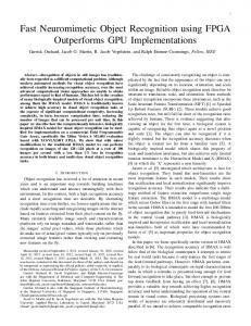
are local evidence potential and clique potential, respectively. The first term ensures that the recovered correspondences are faithful to the data, while the second term encodes our prior assumption that local graphical planarity should be preserved. A graphical depiction of this model is shown in Fig 2(a). The filled-in circles represent the observed image nodes, while the empty circles represent the “hidden” labeling nodes lf . Note that the clique potential in our model differs from its counterparts in [19] and [11] in that we model the spatial interaction of three nodes instead of two neighboring nodes in a pairwise Markov random field [23].

3.3 Implementation The computation of the global optimal solution to the energy function in Eqn. 5 is NP-hard because we need to examine all the possible labeling configurations and compute their energy. The large number of nodes in the graph also calls for faster algorithms like belief propagation (a.k.a sum-product) [23] or graph cut [11]. However, a careful investigation shows that the energy function in Eqn. 5 is not regular or graph-representable [11]. Therefore, standard st-cut algorithm cannot be applied in this case. We propose to use the max-product algorithm for factor graph [12] to solve the MAP-MRF problem. Although the 1 A maximal clique is a triangle in the Delauney triangulation in our case.

Figure 2. (a) MRF; (b) The corresponding factor graph. max-product (or sum-product for marginal distribution estimation) algorithm is an approximate inference algorithm which cannot guarantee the global optimal solution, it has been successfully applied in many Bayesian inference problems in vision, bioinformatics, and error-correcting coding [12, 22]. In Fig 2(b) we illustrate the equivalent factor graph to the MRF. Note that we introduce factor functions Φ(·) of a single variable if they are attached to a single “hidden” node, and factor functions Ψ(·, ·, ·) of three variables if they link three “hidden” nodes. Yedidia et al. [23] show that the belief propagation algorithm is precisely mathematically equivalent at every iteration to the max-product algorithm by converting a factor graph into a pairwise MRF. However, a factor graph representation is preferred in our case because each node in the graph is physically meaningful and the message passing rule can be derived in a straightforward way. 3.3.1 The Max-Product Algorithm Let mi→Φ (li ) and mi→Ψ (li ) denote the message sent from node i to its neighboring function nodes; let mΦ→i (li ) and mΨ→i (li ) denote the message sent from function nodes to node i. The message passing performed by the max-product algorithm can be expressed as follows: 1. Initialize all the messages m(li ) as unit messages. 2. For t = 1 : N , update the messages iteratively variable to local function Y (t) (t+1) mi→Φi (li ) ←− mΨ→i (li ) Ψ∈N (i)

 (t+1) mi1 →Ψi i i (li1 ) ←−  1 2 3

 Y

(t) mΨ→i1 (li1 ) Ψ∈N (i1 )\{Ψi1 i2 i3 } (t)

mΦi

1 →i1

(li1 )

·

We use 4i1 i2 i3 and 4f (i1 )f (i2 )f (i3 ) to denote two matched triangles. The clique potential is defined by

local function to variable (t+1)

mΦi →i (li ) ←− Φi (li ) ³ (t+1) mΨi i i →i1 (li1 ) ←− max Ψi1 i2 i3 (li1 , li2 , li3 ) li2 ,li3

1 2 3

(t)

mi2 →Ψi

(t)

1 i2 i3

(li2 )mi3 →Ψi

1 i2 i3

´ (li3 )

where N (i) is the neighboring function nodes of i. 3. Compute the beliefs and MAP µi (li )

= κΦi (li )

Y

mΨ→i (li )

Ψ∈N (i)

liM AP

=

arg max µi (li ) li

Notice that the variable to local function message mi→Φi (li ) is not involved in the MAP computation explicitly. We list it here for the purpose of completeness. 3.3.2 Model Local Evidence We model the local evidence as a robust function of the flexible template matching distance: ( 2 Rij if Rij ≤ θ 2 1+R γ(i, 1, F ) = ij α otherwise ( 2 θ if Rij ≥ θ 2 1+Rij γ(i, 0, F ) = α otherwise where Rij is the distance defined in Eqn. 1, θ is a predeθ2 fined threshold, and α = 1+θ 2 is the robust parameter. Our robust function is similar to the Geman and McClure function [3] except that we make a truncation at the threshold θ. Local evidence is defined in such a way that γ(i, li , F ) has converse behaviors for li = 0 and li = 1, i.e., when i is labeled as a correct match, the local evidence favors the feature with small matching cost; while when i is labeled as a mismatch, the local evidence favors the feature with large matching cost. 3.3.3 Model Clique Potential The clique potential models the spatial interaction among neighboring features. For objects with small deformations, we assume that the sidedness of the vertices in a triangle is preserved. The sidedness of a triple (i1 , i2 , i3 ) describes their orientation in 2D, i.e., whether the vertices occur in a clockwise (or counter-clockwise) order. As suggested by Ferrari et al. [7], the sidedness constraint is valid for both coplanar or non-coplanar triples and can be used to detect false matches. Such a constraint can be determined by eval− → − → → − uating the sign of the scalar ( i1 × i2 ) · i3 .

ϕ (l , l , l ) = i1 i2 i3 i1 i2 i3 λ if Sign(4i1 i2 i3 ) = Sign(4f (i1 )f (i2 )f (i3 ) )     and li1 = li2 = li3 = 1;  5λ if li1 or li2 or li3 is 0;   20λ if Sign(4i1 i2 i3 ) 6= Sign(4f (i1 )f (i2 )f (i3 ) )    and li1 = li2 = li3 = 1

where λ is a parameter to measure the consistency. We favor topologically consistent matches, while enforce strong penalty for matches which violate the sidedness constraint. We also apply less penalty for an ambiguous matching clique (one or more vertices are labeled as mismatches in one triangle).

4. Experimental Results Feature Template Matching: Our first example is to show the process of finding mutually best local matches and flexible template matching. In Figure 3, the green dots are the features which have found their mutually best matches, i.e., possible template centers. Although significant feature clusters on the background have been removed (we do not show the original SIFT features here because they are very dense), we see quite a lot of errors in the putative matches. This can be observed partly from the green dots scattered outside of the object region in the input image. After flexible template matching, the surviving feature template centers are shown in red dots. We can see that flexible template matching effectively gets rid of all except one (on the border of the “algorithms book”) false correspondences in this case. In Figure 4 we show details of the template matching process. We demonstrate the matching of a matched pair A and A0 , and a mismatched pair B and B 0 (which are shown in red crosses). For corresponding features in the model view and input view, their 5- and 8-nearest neighbors are shown to the right of the figure. Feature A finds very similar surrounding patches in A0 that are also angular order preserving. However, B is supported very weakly by its neighbors. As a result, B is detected as a false match. Object Detection in Cluttered Scenes: Next we show results of the global matching step. The surviving features after the first step are subject to a global topology verification procedure in which the max-product algorithm is performed to search for the maximal subgraph in the input view. Figure 5 shows some object detection results in highly cluttered scenes. For each input view, we show the matched graph on the model view. Red lines in the image signal wrong matches left over by the flexible template matching. They are detected because their removal will give a maximal subgraph that is also faithful to the data.

B

A

A’

B’ Figure 3. Flexible feature template matching. Green dots: mutually most similar features. Red dots: correspondences found by template matching. Figure 5. Detection in cluttered background. TA TA’ TB TB’

Figure 4. Matching by dynamic programming. Solid lines: good matches; dashed lines: weak matches. Non-rigid Object Detection: The proposed object detection framework can also be applied to non-rigid objects. In Figure 6 we show the detection result of a magazine. We manually introduce severe non-rigid distortions in the test views which do not follow any explicit transformation. It can be seen that our algorithm has successfully captured the object shape even under a cluttered background, with severe distortion and partial occlusion. Object with Repetitive Patterns: In Figure 8, we show a very challenging sequence in which the interested object has repetitive patterns and is occluded by another object. We show the object detection results at different scales and orientations. An Assumption Violation Case: Finally Figure 7 shows an example of object detection when our 2D spatial ordering assumptions are violated. The scene consists of a marker pen in front of a textured background. Due to the picket-

and-fence effect, the ordering constraints of some features are obviously violated. For example, the pen is to the left of the “multiple view geometry book” in the model view, while to the right of the same book in the test view. Features highlighted by two circles will have their local ordering constraint violated. However, our program is robust enough to detect these violations and show them in red lines. Meanwhile, the rest of the scene is accurately detected. Five parameters need to be set in our algorithm: one threshold for flexible template matching, m and n for spatial nearest neighbors selection, θ and λ for local evidence and clique potential modeling. We choose these parameters empirically and all the experiments shown here use the same set of parameters. The max-product algorithm has shown to be very efficient for the graph matching problem. For a graph with hundreds of nodes, it takes only 10 to 20 iterations for the beliefs to converge. We have tested our algorithm on a variety of objects and extensive experiments show that the proposed method is able to detect object in cluttered scenes effectively and efficiently. Our system currently runs at 2 frame-per-second on 320x240 images.

5. Conclusion We have presented a two-step framework for general 3D object detection in cluttered scenes with unknown camera poses. We demonstrated that false matches between features are progressively detected by data evidence and 2D ordering constraints in both a local and a global scale. Ex-

Figure 6. Nonrigid object detection.

Figure 8. Detecting objects with repetitive patterns. [7] V. Ferrari, T. Tuytelaars, and L. Van Gool. Integrating multiple model views for object recognition. In CVPR, 2004. [8] W. T. Freeman and E. H. Adelson. The design and use of steerable filters. PAMI, 13(9):891–906, 1991. [9] I. K. Jung and S. Lacroix. A robust interest point matching algorithm. In ICCV, 2001. [10] T. Kadir and M. Brady. Scale, saliency and image description. IJCV, 45(2):83–105, 2001.

Figure 7. An assumption violation case. periments on various objects have shown great promise in applying the proposed methods to real world applications. In our future work, we would like to increase the usability of the proposed method. We are interested in developing real time object detection systems. Currently the most time consuming part of our program is SIFT feature detection. We plan to investigate other feature detectors and efficient algorithms.

Acknowledgement We would like to thank Prof. David Lowe for kindly providing the SIFT source code.

References [1] S. Agarwal and D. Roth. Learning a sparse representation for object detection. In ECCV, pages 113–127, 2002. [2] Y. Amit, D. Geman, and K. Wilder. Joint induction of shape features and tree classifiers. PAMI, 19(11):1300–1305, 1997. [3] M. J. Black and A. Rangarajan. On the unification of line processes, outlier rejection, and robust statistics with applications in early vision. IJCV, 19(1):57–91, 1996. [4] A. Cross and E. Hancock. Graph matching with a dual-step EM algorithm. PAMI, 20(11):1236–1253, 1998. [5] R. Fergus, P. Perona, and Z. Zisserman. Object class recognition by unsupervised scale-invariant learning. In CVPR, 2003. [6] V. Ferrari, T. Tuytelaars, and L. Van Gool. Wide baseline multiple view correspondence. In CVPR, pages 718–725, 2003.

[11] V. Kolmogorov and R. Zabih. What energy functions can be minimized via graph cuts. PAMI, 26(2):147–159, 2004. [12] F. R. Kschischang, B. J. Frey, and H.-A. Loeliger. Factor graphs and the sum-product algorithm. IEEE Transactions on Information Theory, 47(2):498–519, 2001. [13] D. G. Lowe. Distinctive image features from scale-invariant keypoints. IJCV, 60(2):91–110, 2004. [14] K. Mikolajczyk and C. Schmid. A performance evaluation of local descriptors. In CVPR, 2003. [15] P. Moreels, M. Maire, and P. Perona. Recognition by probabilistic hypothesis construction. In ECCV, 2004. [16] Y. Ohta and T. Kanade. Stereo by intra- and inter-scanline search using dynamic programming. PAMI, 7(2):139–154, 1985. [17] F. Rothganger, S. Lazebnik, C. Schmid, and J. Ponce. 3D object modeling and recognition using affine-invariant patches and multiview spatial constraints. In CVPR, 2003. [18] F. Schaffalitzky and A. Zisserman. Multi-view matching for unordered image sets, or How do I organize my holiday snaps? In ECCV, 2002. [19] J. Sun, N. N. Zheng, and H. Y. Shum. Stereo matching using belief propagation. PAMI, 25(7):787–800, 2003. [20] S. Umeyama. An eigendecomposition approach to weighted graph matching problems. PAMI, 10(5):695–703, 1988. [21] L. Van Gool, T. Moons, and D. Ungureanu. Affine photometric invariants for planar intensity patterns. In ECCV, pages 642–651, 1996. [22] M. J. Wainwright and M. I. Jordan. Graphical models, exponential families, and variational inference. Technical Report 69, Department of Statistics, University of California, Berkeley, 2003. [23] J. S. Yedidia, W. T. Freeman, and Y. Weiss. Understanding belief propagation and its generalizations. Technical Report 2001-22, MERL, 2001.