Object-Oriented Bond-Graph Modeling of a Gyroscopically Stabilized Camera Platform Robert T. McBride Raytheon Missile Systems P.O. Box 11337, Bldg. 805, M/S L-5 Tucson, AZ, 85734-1337, USA
[email protected]
Keywords : Dymola, object-oriented physical system modeling, graphical modeling, gyroscope. Abstract The paper demonstrates, by means of an example of a gyroscopically stabilized platform, the method in which bond-graph models can be used in an object-oriented manner to create an overall physical system model. The gyroscopically stabilized platform was chosen as an example because of its complex mechanical interconnections, electrical/mechanical inter-disciplinary nature, and the necessity to create the model in a threedimensional setting. The paper discusses in detail the bond-graph models of each of the object-oriented system sub-components as well as the model of the overall system. The model is implemented using a new bondgraph library implemented in Dymola, which is described in the companion paper: Object-Oriented Modeling of Complex Physical Systems Using the Dymola BondGraph Library, also presented in this conference. The paper demonstrates that the tools/methods presented indeed offer the capability to solve serious engineering problems.
INTRODUCTION Object-oriented tools that model systems of multiple engineering domains are not yet common in the engineering workplace. One of the primary reasons for this is that the tools that do exist for these applications are not developed to the point of being able to solve industrial problems. Often these tools are able to capture only a small fragment of the engineering modeling discipline, forcing the design engineer to either use a wide variety of tools for a single system, or to create large sections of C++/FORTRAN code that are not reusable and difficult to alter for new designs. Bond-graphs can provide the engineering community with a single set of tools that cross multiple engineering domains. As well, bondgraphs can be used in an object-oriented modeling fashion allowing bond-graph models/sub-models to be used in a
François E. Cellier University of Arizona P.O. Box 210104, Tucson, AZ, 85721-0104, USA
[email protected]
plug and play manner. The object-oriented system mo del then consists of connecting many sub-models together in a bond-graph fashion where each sub-model contains a bond-graph that can easily be altered for new designs, allowing the design engineer to experiment with many variations of the same system prior to laboratory testing. Detailed modeling of industrial systems can give a design team insight into the behavior of a system well before the system is manufactured. The ability to model these systems quickly and correctly gives the design team the advantage of being able to test many variations of the same system, thus allowing the team to choose the optimal design for their specific needs. Using bondgraphs in an object-oriented fashion provides the engineering community with a powerful design technique. The ability of bond-graphs to cross multiple engineering domains, and their natural object-oriented structure, gives the engineering community an essential tool that can quicken the pace of system design and development from the proposal phase through t o design completion [1]. The model of a gyroscopically stabilized platform given in this paper makes use of the bond-graph model of a two-gimbaled gyroscope. The gyroscope model is used four separate times in the stabilized platform model. The gyroscope model is used in three instances as a gyroscope model to sense the roll, pitch, and yaw of the platform, and once as a camera model that can be commanded to rotate in the roll, pitch and yaw directions. The mathematics of the camera are identical to the mathematics of the gyroscope; however the method under which they are used is different.
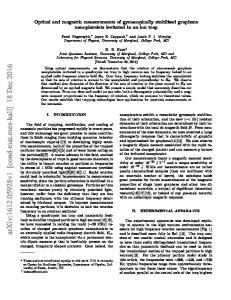
THE GYROSCOPE MODEL The rotational axis definitions of the two-gimbal gyroscope are shown in figure 1, where θ , φ , and ψ , the three Euler angles, are the generalized coordinates of the system. The moment of inertia of the rotor about the symmetry axis æ is denoted as C , and A is the moment of inertia of the rotor about any transverse axis through the point O. The moments of inertia of the inner gimbal
about the axes î, ç, and æ, are denoted by A′ , B′ , and C ′ , respectively. The moment of inertial of the outer gimbal about the inertial axis Z is denoted by C ′′ . The distance l shown in figure 1 is zero for the purpose of this paper. These inertia/axis definitions are consistent in each of the gyroscope bond-graphs and in the camera bond-graph.
bond-graph is the added integration of θ& to produce θ . This increases the order of the system from three to four. Figure 3 shows the Dymola implementation of this bond graph using the Dymola Bond-Graph Library.
Figure 1. Axis Definitions of the Two-Gimbal Gyroscope The bond-graph of the gyroscope is shown in figure 2. A detailed development of this bond-graph structure is offered in McBride and Cellier [2]. This bond-graph structure can be implemented in Dymola using the Dymola Bond-Graph Library [3]. Figure 3. Dymola Implementation of the Gyroscope Bond-Graph Although the bond-graph of figure 3 is more difficult to read than the representation given in figure 2, the Dymola simulation tool [4] is able to create executable code from the bond-graph shown in figure 3, whereas figure 2 serves only as a diagram. Figure 3 shows three signal connectors at the left of the diagram, labeled Seθ , Seψ , and Seφ . Here effort source signals can be connected to the model from the outside. The output connector, shown at the bottom right, outputs a six-element vector containing values Figure 2. Bond-Graph of the Two-Gimbal Gyroscope The signal flow arrows shown in figure 2 are momentum signals. The modulated gyrators are signaled by the moments of different I elements. Also implied in the
θ& , θ ,ψ& ,
ψ , φ& , and φ , making these signals available to models outside the gyroscope model. Dymola offers three windows for creating a model: the diagram window, the equation window, and the icon window. Figure 3 shows only the diagram window. Not all of the connections are shown in figure 3. For example
the output connector does not seem to be connected at all. This is because these connections were programmed in the equation window, since it was more convenient to do, and since it prevents the diagram from being cluttered up with lots of signal paths. Although it is possible to use bond-graphic connectors, it was chosen here to use signal connectors, because signals and block diagrams are more convenient to use at the hierarchically higher control level. When the gyroscope bond-graph is used as an object-oriented model, i.e., when it is dropped into a larger model, the gyroscope model is represented by its icon. Only its input/output connections and icon are shown. Embedded in the bond-graph of figure 3 is the ability to manipulate the model from the outside in the following ways: ♦ Add initial conditions to any of the state variables,
θ& , θ ,ψ& , ψ , φ& , and φ . ♦
Define the moments of inertia of each of the inertial elements. This gives the modeler control of these parameters from outside the model. Figure 4 shows an example of the gyroscope bondgraph being used in a plug-and-play manner. Here the bond-graph gyroscope model of figure 3 is represented by its iconic representation, which is how hierarchical models are built in Dymola. The bond-graph of the gyroscope is one layer below the gyroscope icon shown in figure 4. The inputs to the model shown in figure 4 are roll, pitch and, yaw. The roll, pitch, and yaw signals are those of the platform body used to command the modulated efforts inside the gyroscope bond-graph. A position orientation between the platform and the gyroscope is implied, since the roll, pitch, and yaw signals have been attached to the gyroscope in a specified manner.
Figure 4. Gyroscope Bond-Graph is dropped into a Larger Model.
The effort source signals are scaled by the moments of inertia of each of the gyro axes divided by the moment of inertia of the platform about the same axis. This scaling ensures that the gyroscope inputs are of the correct magnitude. The scaling on Seφ is a bit more complicated then a simple scale factor, since the moment of inertia about the inertial axis Z, of figure 1, changes as the angle θ changes. As seen in figure 4, the angle θ is fed into the calculation of the
Seφ scale factor. The Seφ
scale factor is given by the equation:
mSeφ = SePitch
C′′ + C′ cos 2 θ + ( A + B′) sin 2 θ I Platform_ Pitch
The model shown in figure 4 orients the gyroscope such that a yaw platform motion is sensed by movement in the gyroscope Euler angle ψ . A subtle implication to the way that the gyroscope bond graph is created is that the initial angle θ , as defined by figure 1, should be set at 90°. Figure 4 shows only the yaw gyroscope. Two more similar models were created to sense the pitch and roll motion of the platform. These three gyroscopes, each in their respective orientations, are combined in figure 5 to create an inertial-rate sensor block. Connected to each of the gyros of figure 5 is a sensor block. This block subtracts out gyro initial conditions so that the platform motion is the only remaining value in each respective signal. This block also contains discrete time delays to simulate the delay necessary to perform these operations in an on-board computer or actual sensor. The output of the sub-model shown in figure 5 is again a six-element vector. This output vector contains values of roll rate, roll, pitch rate, pitch, yaw rate, and yaw.
Figure 5. Inertial-Rate Sensor, Three-Gyro Block.
(1)
These values are then fed back into the platform motion controller to stabilize the platform.
THE CAMERA MODEL
element, as shown in figure 7. The model shown in figure 7 represents a single channel of the platform. This bondgraph model will be used in three separate instances to represent the roll, pitch and yaw motion of the platform.
The gyroscope bond-graph model was also used to simulate a two-gimbal camera. The camera equations are identical to the gyroscope equations, but the camera is used in a different fashion. The camera is commanded to an inertial position. It is expected that the camera be fixed on an inertial point regardless of the body motion of the platform that the camera is fixed to. The camera model is shown in figure 6.
Figure 7. Platform Channel Bond-Graph
Figure 6. Camera Stabilization.
A flow sensor f element [3] was used to record the actual platform rates and positions for each axis. The actual motion of the platform are compared to the gyroscopically-sensed platform motion. Figure 8 shows the three separate channels of the platform connected together to form the full platform model. Each channel contains the simple bond-graph model of figure 7.
As shown in figure 6, the gyroscope bond-graph model represents the dynamics of the camera model. The camera model shown in figure 6 orients the camera to the platform similar to the gyroscope of figure 4. A yaw camera command will cause a φ camera rotation, a pitch camera command will cause a θ camera rotation, and a roll camera command will cause a ψ camera rotation. The camera is stabilized with state feedback to minimize the error between commanded and measured positions. As in the gyroscope models, the initial angle θ should be set at 90°. Figure 6 shows that this rotation is subtracted from the measured camera pitch angle. Thus this rotation is transparent to the outside world. A command of zero will keep the camera pointed at an angle θ of 90°, where θ is defined by figure 1.
THE PLATFORM MODEL The gyroscope models are used to stabilize the motion of a platform. The camera model will also be attached to this platform. The platform model is a very simple bond-graph model that is also used in an objectoriented fashion. This simple model consists of an effort source connected to a 1-junction connected to an inertia
Figure 8. Platform Model. The system is set up to give separate pitch, yaw, and roll motion. As can be seen in figure 8, the model is set up for a position command input. The gyroscopicallysensed body rates, and body positions are fed into the platform controller to stabilize the platform body motion. The sensed body rates and positions are output from the inertial rate sensor of figure 5. The outputs of the
platform model are the three torques that are generated by the platform controller, labeled Platform_Torques, and the actual platform position and rates, labeled Platform Rates and Positions. The three torque commands are sent in as Se_Roll, Se_Pitch, and Se_Yaw to the inertial-rate sensor of figure 5. This is to ensure that the efforts used to move the platform are the same efforts used to excite the gyroscopes.
platform motion. If the gimbaled camera had been left open loop there would have been no need to take into account the platform motion since the platform would not have been able to induce a torque on the camera. However, since the camera position is closed loop with its reference to the platform body, it is necessary to take into account the body motion.
THE STABILIZED PLATFORM MODEL The Inertial-rate sensor model of figure 5 is connected to the platform model of figure 8, to create the gyroscopically stabilized platform model shown in figure 9.
Figure 10. Stabilized-Platform and-Camera Combined. The outputs of the stabilized platform model are passed to the outside as well as the inertial camera angular positions.
THE COMPLETED MODEL Figure 11 shows the complete model. This model is connected to outside platform position commands and camera position commands.
Figure 9. Gyroscopically Stabilized Platform. Figure 9 shows the platform position commands coming into the platform model. A position controller changes the platform position commands into torques acting on the platform body. These same torque values are passed to the inertial-rate sensor block model of figure 5. The outputs of the rate sensor block are fed back into the platform controller to close the loop. The outputs of the gyroscopically stabilized sub-model are the actual platform motion, used for simulation purposes, and the gyroscopically-sensed platform motion. Both position information and rate information are output for each of the three inertial axes.
THE COMBINED CAMERA MODEL
PLATFORM
AND
The stabilized platform model of figure 9 and the camera model of figure 6 are combined in figure 10. As shown in figure 10, the sensed platform motion of roll pitch and yaw is subtracted from the inertial camera commands of roll, pitch and yaw to cause the camera to point at the commanded inertial angles regardless of the
Figure 11. Complete Model. The position commands are shown as signal boxes coming in at the left of figure11.
The platform is made up of three instances of an effort source connected to an inertia element. The rest of the complete model consists of the supporting mathematics needed to exercise the gyroscope bond-graph models. The overall model demonstrates that a bond-graph model can be used as an object-oriented element to complete a model of greater complexity. In so doing, the modeler can save time and effort needed to create larger, more complex models.
commanded to pitch, yaw, and roll in a sinusoidal motion. This commanded sinusoidal motion is described in figure 12. As seen in figure 12, roll, pitch, and yaw were commanded to react to different magnitude and frequency sine waves. The gyroscopes sense the platform motion. This sensed response is shown in figures 13-15 for pitch, roll, and yaw, respectively. The small transient at the beginning of the plots 13-15 is due to the integrators/timedelays charging up. This transient dies off quickly however. Platform Commanded Angular Pos. 15 Roll Pitch Yaw
10
5 Angle (deg.)
This is the completed model. The heart of this gyroscopically stabilized platform model is a bond-graph gyroscope model, and a simple bond-graph of an effort signal connected to an inertial element. Both of these bond-graph models were used in multiple instances to complete the overall model. The bond-graph gyro model is used in four separate instances: 1. Gyroscope one senses the platform-yaw and yaw rate. 2. Gyroscope two senses the platform-pitch and pitch rate. 3. Gyroscope three senses the platform-roll and roll rate. 4. Gyroscope four is used as a camera set in two gimbals.
0
-5
-10
-15
0
5
10
15
Time (sec.)
DYMOLA SIMULATION AND RESULTS
Gyros 400 900 40 80 40 75 1500
Camera 1800 3600 160 320 160 300 0
Table 1. Values for the Simulation Run. properties were arbitrarily chosen as Ipitch = 5E4, Iyaw = 4E4, and Iroll = 3.5E4. The sensor delays were set a 1kHz. The simulation run consisted of commanding the camera to a specified point and then commanding the platform to move. The camera, initially at 0° about all three inertial axes, was commanded to maintain a constant inertial position of 57.3° about all three inertial axes. These inertial camera angles are expected to remain unchanged while the platform is commanded to oscillate through a series of maneuvers. The platform was
As seen in figure 13 the pitch sensed response matches the commanded very well. The error is less than 1° and is considered negligible. Platform: Pitch 10 Pitch Angle (deg. )
A C A′ B′ C′ C ′′ ψ& 0
Figure 12. Platform Position Commands.
Gyro-Sensed Commanded
5 0 -5 -10
Pitch Angle Error (deg. )
Dymola was used to simulate the camera platform model. The gyro and camera mass properties were arbitrarily chosen as shown in table 1. The platform mass
0
5
0
5
10
15
1 0.5 0 -0.5 -1 Gyro-Sensed - Commanded -1.5
10
15
Time
Figure 13. Pitch Gyro Output. The roll gyro response of figure 14, however, shows a considerably larger error, on the order of 7° at times. This is due to the high frequency at which the platform was asked to roll. The roll gyro senses a considerable
amount of overshoot., more so than either the pitch gyro or the yaw gyro shown in figure 15.
pitch motion of the camera in an inertial frame. Once the initial transient dies off, the error in the pitch channel never gets bigger than 1°.
Platform: Roll Camera: Pitch
Gyro-Sensed Commanded
10
80
0 -10 -20
0
5
10
15
Pitch Angle (deg. )
Roll A ngle (deg.)
20
60
20 0
Roll A ngle Error (deg.)
Gyro-Sensed - Commanded 5 0 -5 -10
0
5
10
15
Time
Figure 14. Roll Gyro Output.
Pitch: Camera Inertial Error (deg.)
-20 10
Camera Body Pos. Commanded Platform Body Motion
40
0
5
10
15
60 40 20 0 Camera Cmnd. - Camera Pos. - Body Mtn. -20
0
5
10
15
Time
Figure 16. Camera Pitch Response Figure 15, the yaw gyro output, shows an intermediate amount of error when compared to the roll channel or the pitch channel. This is also due to the relatively high frequency moving the platform. Platform: Yaw Gyro-Sensed Commanded
10 0 -10 -20
0
5
10
80 Roll A ngle (deg.)
4 Yaw Angle Error (deg.)
Camera: Roll
15
Gyro-Sensed - Commanded 2 0 -2 -4
60
0
5
10
15
Time
Figure 15. Yaw Gyro Output. Figures 16-18 show the response of the two-gimbal camera in pitch, roll, and yaw, respectively. The camera was initially set at 0° for all three axes. At time 0, the camera commands a step to 57.3° in all three directions. The camera responds and then tries to maintain an inertial position by subtracting out the sensed pitch, roll, and yaw components of the body motion. Figure 16 shows the camera response to both the command in the pitch direction and the pitch body motion. Also shown is the actual body motion for reference. The error shown in figure 16 is the error of
Camera Body Pos. Commanded Platform Body Motion
40 20 0 -20
Roll: Camera Inertial Error (deg.)
Yaw Angle (deg.)
20
The camera response in the roll channel is somewhat more interesting. The body motion is of a higher frequency and causes the camera to have to respond more quickly. Even after the transient of the roll-sensed body motion has died out, there is some error remaining. This error is due to cross coupling between the cameracommanded roll and the camera-commanded yaw. The cross coupling between these two channels is mostly evident in the camera yaw response shown in figure 18.
0
5
10
15
60 40 20
Camera Cmnd. - Camera Pos. - Body Mtn.
0 -20
0
5
10
15
Time
Figure 17. Camera Roll Response Figure 18 shows the camera yaw response. As in both the camera pitch and roll responses, the initial transient dies out rapidly. However, the camera yaw response is somewhat different from the pitch and roll responses in that the channel cross coupling is very evident. The channel-to-channel cross coupling could be
reduced by feeding the platform rates into the camera position controller.
[4] DYMOLA Dynamic Modeling Laboratory, World Wide Web page http://www.Dynasim.se.
Camera: Yaw
Yaw Angle (deg.)
80 60 40
0 -20
Yaw: Camera Inert ial Error (deg.)
Camera Body Pos. Commanded Platform Body Motion
20
0
5
10
15
60 40 20
Camera Cmnd. - Camera Pos. - Body Mtn.
0 -20
0
5
the Dymola Bond-Graph Library,” Proc. ICBGM’03 Conference, Orlando, Florida.
10
15
Time
Figure 18. Camera Yaw Response
CONCLUSIONS The paper has demonstrated how bond-graph models of physical devices can be embedded in an overall control architecture in an object-oriented fashion. In the past, several researchers have used bond graphs in an object-oriented fashion by creating so-called “word bond graphs.” However, these word bond graphs were used only to communicate concepts, not as simulation tools. The Dymola modeling framework enables the modeler to convert hierarchical bond-graph models into software objects that can be integrated into larger entities, and that can be used in simulation experiments. A gyroscopically stabilized platform was used in this paper to demonstrate the generality of the approach to object-oriented bond-graph modeling of physical systems, and to show that the tools available to this end are powerful enough to deal with complex industrial processes.
REFERENCES [1] Brück, D., H. Elmqvist, S.E. Mattsson, and H. Olsson (2002), “Dymola for Multi-Engineering Modeling and Simulation,” Proc. Modelica’2002 Conference, Munich, Germany, p. 55:1-9, http://www.modelica.org/Conference2002/papers/p07_Br ueck.pdf . [2] McBride, R.T., and F.E. Cellier (2001), “A BondGraph Representation of a Two-Gimbal Gyroscope,” Proc. ICBGM’01 Conference, Phoenix, Arizona, p. [3] Cellier, F.E., and R.T. McBride (2003), “ObjectOriented Modeling of Complex Physical Systems Using