3
I&S
OBJECT-ORIENTED ENVIRONMENT FOR ASSESSING TRACKING ALGORITHMS Emanuil DJERASSI and Pavlina KONSTANTINOVA
1. Introduction One way to alleviate the complex problem of designing, assessing, and implementing tracking algorithms is to provide the designer with an environment facilitating the creation of various test scenarios, assisting the implementation of algorithms, and evaluating their performance. Such an environment is a complex software program, which could be simplified by using object-oriented design and programming. The overall program organization can be improved by unifying data and functions that operate on the data. Both users and designers are interested in assessing and comparing the numerous target tracking methods and algorithms developed in recent years. Usually, for this purpose a dynamic situation is modeled by simulating signals from moving targets and false alarms. On the base of these signals, the target tracking algorithms initiate and estimate target tracks. This task is complex because of the uncertainty of the dynamic situation and the explosive increase of the computational load corresponding to the number of targets, typical for most tracking algorithms. It often happens that new algorithms differ only slightly from those already programmed and tested. Also, it is sometimes necessary to add new properties to the dynamic situation. These processes can be alleviated using the methods of the Object-Oriented Programming (OOP), creating a set of classes that implement the basic data structures and routines used in the simulation environment. 2. Problem formulation The environment consists of four main parts, organized in the hierarchy presented on Figure 1.
INFORMATION & SECURITY. An International Journal, Vol. 9, 2002, 93-106.
94
Object Oriented Environment for Assessing Tracking Algorithms
The Organization Part allows the user to choose a tracking algorithm and to control the mode of its implementation. Using the polymorphism, the user needs only to create or change a virtual tracking function and then to define an object of its class. This part organizes two modes of work: single and Monte Carlo mode. In single mode the following steps are performed: Simulation of the dynamic situation;
Tracking algorithm implementation (data processing);
Result visualization. These steps are repeated on each scan. The Monte Carlo mode consists of two steps: Accumulating statistical data by iteratively performing the first two steps of the single mode;
Comparison of result and visualization.
The Simulation Part provides methods for simulating target movements, environment characteristics and sensor parameters. The Data Processing part contains specific tracking algorithms, programmed by the user. The Vector-Matrix Computation part is an auxiliary part, providing a variety of classes and methods for matrix computations, which are widely used in target tracking algorithms. Organization
Simulation
Data Processing Target Tracking
Vector-Matrix Computations
Figure 1: Components of the software environment
95
Emanuil Djerassi and Pavlina Konstantinova
3. Description of the classes 3.1.
Classes for program organization
The multiple parameters characterizing a dynamic situation can be appropriately presented in a class Scenario and the flags controlling different modes and their parameters – in a class Control. The parameters for MonteCarlo analysis and the functions for MonteCarlo mode implementation are included in class MonteCarlo. These three classes are parents of an abstract class TrackingAlg. The objects of class TrackingAlg have direct access to multiple parameters and flags. On the other hand, the class TrackingAlg has three pure virtual functions: Tracking, ShowScenario and ShowResult. The particular tracking algorithms, as derived from class TrackingAlg, must define these pure virtual functions. Thus, the program code of the main part of the program for all tracking algorithms will be the same. Figure 2 shows the hierarchy of these classes. New classes could be added on the place of the dashed line.
// class TrackingAlg- abstract class with pure virtual functions class TrackingAlg: MonteCarlo {
class
SCENARIO,
class
CONTROL,
class
public: virtual void Tracking();)=0; virtual void ShowScenario()=0; virtual void ShowResult()=0;
}; class JPDAF: public TrackingAlg public: virtual void Tracking(); virtual void ShowScenario(); virtual void ShowResult(); }; {
class NN: public TrackingAlg
{
public: virtual void Tracking(); virtual void ShowScenario(); virtual void ShowResult();
};
In this case, the links between member-functions and objects are of the type “late binding,” i.e., on run time. Depending on the particular algorithm, the pointer FilterObjPtr will be initialized by the address of the object from the particular class. For example, the source code for two algorithms JPDAF and NN is: if (TypeOfProcessing==1) FilterObjPtr = new JPDAF; if (TypeOfProcessing==2) FilterObjPtr = new NN;
96
Object Oriented Environment for Assessing Tracking Algorithms
Similarly, new classes can be introduced for newly developed algorithms. The source code of the main program in single mode is: switch (FlagStage) { case 1: FilterObjPtr->ShowScenario(); FilterObjPtr->Tracking(); break; case 2: FilterObjPtr->ShowResult(); break; default: break; } // end of switch
The source code of the main program in MonteCarlo analysis mode is FilterObjPtr->MonteCarloRun(); And because in class MonteCarlo the function Tracking is declared as virtual in runtime, the tracking function corresponding to the chosen algorithm will be selected. This is an example of polymorphism, as the same code implements different methods according to the type of FilterObjPtr. Depending on the work stage, the methods ShowScenario and the tracking algorithm Tracking or the method ShowResult are implemented. Thus, the addition of a new algorithm is reduced to defining a new class derived from the abstract class TrackingAlg and defining its particular virtual methods Tracking, ShowScenario and ShowResult. The main part of the program can remain unchanged.
class SCENARIO
class CONTROL
class MONTE CARLO
abstract class TrackingAlg
class NN
class JPDAF
----
Figure 2: Class hierarchy
Emanuil Djerassi and Pavlina Konstantinova
3.2.
97
Classes for simulation
The data defining some specific dynamic situation (scenario) is initially entered from a file. Each simulated target requires data on initial coordinates, velocity and movement direction, and the maneuvering targets need also information regarding initial and final times of the maneuver, acceleration during the maneuver, etc. Based on the data for each sensor observation, current coordinates are computed and stored in order to check later the measures of performance of the tracking algorithm. It is useful to define a class ClsTarget unifying all that data for a target and the functions dealing with it.5,6 The basic behavior characteristics of a target moving according to specific rule are implemented through the class method MoveToNextPosition. In spite of the fact that the method uses multiple data for each object, it is not necessary to write them because the method has direct access to all the data for the object. The other two methods ReadTargetData and CoordInitializing are used at the beginning for target data initialization. The description of this class is: class ClsTarget // Information about target int Label1 ; int Type1; float Xi,Yi; // Initial Coordinates float WI ; // Current Velocity float PSIi ; // Initial Velocity float Azi ; // Initial Heading float X,Y,Z; // Current Cartesian coordinates float DDot,D,Azimuth,Epsilon; // Current Polar coordinates int InitialScan; int NTrSegments; public: // Methods for the class void ReadTargetData(FILE *FileIn); void CoordInitializing(); void MoveToNextPosition(); // friend functions, which use Targets’ data friend void DefineDetectedTargets(Float Pd, int & NumberOfDetectedTargets, IntArrTarg DetectedTargets); friend int DataPreparationForCurrentScan(); friend float RSE(int itr, int jr) ; friend class ClsMeasurement; } ; // end of class ClsTarget {
98
Object Oriented Environment for Assessing Tracking Algorithms
Another essential group of data describes the simulated measurements or the socalled “raw data.” The raw data is calculated on the base of the data for the moving targets from the objects of the class ClsTarget. For this data it is useful to define a class ClsMeasurement. The function DataPreparationForCurrentScan is declared as a friend function for both classes - ClsMeasurement and ClsTarget. In this function, the measurements “received” on the current scan are computed. According to the specific sensor parameters, the errors of the measurements are simulated. According to the probability to detect correctly, the number of detected targets is defined. The method Noising of the class ClsMeasurement uses the data of the detected target to generate the corresponding measurement. The description of this class follows: class ClsMeasurement { private: int Label1; float X,Y,Z; float Range, Azimuth, float Dopler,Elevation; int Busy; public: void Noising(ClsTarget & ob); friend int DataPreparationForCurrentScan(); };
3.3.
Classes for tracking algorithms
3.3.1 Theoretical background In general, a track is a set of measurements from the same target at different times. However, in most tracking algorithms the track is approximated for each time by a difference equation in the form:3
x(k 1) F (k ) x(k ) G(k )u(k )
(1a)
where x(k ) is a n-dimensional target state vector at time k , which consists of the quantities to be estimated, and F is a transition matrix, G is a control matrix, and u is a control vector. x(k 1) is the prediction of the state vector for time (k 1) . The measurement vector received from the sensor is:
z(k ) Hx(k )
(1b)
Because of the measurement errors and false alarms, the real state vector x is never known. Instead, we have to work with its estimation xˆ . The process of estimating is
Emanuil Djerassi and Pavlina Konstantinova
99
usually called filtering, and the correspondent algorithms are called filters. Nowadays, the common filters used for this purpose are based on the Kalman filter. 3.3.1.1. Linear Kalman filter When equations (1a) and (1b) are linear, the linear Kalman filter is used. The basic form of the this filter is:
xˆ(k 1 | k ) F (k ) xˆ (k | k ) G(k )u(k )
(2a)
zˆ(k 1 | k ) H (k 1) xˆ(k 1 | k )
(2b)
(k 1) z(k 1) zˆ(k 1 | k )
(2c)
P(k 1 | k ) F (k ) P(k | k ) F (k )'Q(k )
(2d)
S (k 1) H (k 1) P(k 1 | k ) H (k 1)' R(k )
(2e)
W (k 1) P(k 1 | k ) H (k 1)' S (k 1) 1
(2f)
xˆ (k 1 | k 1) xˆ(k 1 | k 1) W (k 1) (k 1)
(2g)
P(k 1 | k 1) P(k 1 | k ) W (k 1)S (k 1)W (k 1)'
(2h)
where xˆ is the estimation of the target state vector, z is the measurement vector, H is the measurement matrix, W is the gain matrix, S is the innovation covariance matrix, Q is the noise covariance matrix, R is the measurement covariance matrix, is the innovation vector, and P is the covariance matrix. 3.3.1.2 Nonlinear (Extended) Kalman filter When equations (1a) and/or (1b) are nonlinear, the Extended Kalman Filter is used. Its equations are the same as the equations of the Linear Kalman Filter (2a-2h), but the matrices F(k) and H(k) are Jacobians, based on the first order Taylor expansion of the nonlinear functions (1a) and (1b) respectively. Hence, the nonlinear filter estimation can be reduced to a linear filter estimation after the Jacobians are calculated. 3.3.1.3 Probabilistic Data Association (PDA) filter When the observations from a single target are mixed with clutter, the Probabilistic Data Association filter is applied instead of the classic Kalman filter.4 It is also called “all neighbors method” because the updated estimate for a track contains contributions from all N observations within the gate of track i . The probability of the hypothesis H j ( j 1,2,...N ) that the observation j is a valid return for the track i is proportional to the likelihood function g ij :
100
Object Oriented Environment for Assessing Tracking Algorithms
g ij
e
d ij2 2
2 M 2
(3)
, Si
where d ij2 ijT S i1 ij , ( ij is measurement residual for track according to (2c) ). Then pij' N 1 PD g ij ,
i and measurement j
j 1,2,...,N
(4)
where is extraneous return density, PD is detection probability. The probabilities ( pij ) associated with the N+1 hypotheses (that can be formed) are computed through the normalization equation:
p ij
p ij'
(5)
N
p il'
l 0
The residual for use in the Kalman Filter update equation is a weighted sum of the residuals associated with the N observations: N
~ y i (k ) pij ~ y ij (k ) ,
(6)
j 1
where
yij (k ) y j (k ) Hxˆ i (k | k 1) y j (k ) = observation
j received at scan k .
The covariance P is updated according to the equations:
P(k | k ) P o (k | k ) dP(k )
(7)
where
and
P o (k | k ) pi 0 P(k | k 1) (1 pi 0 ) P* (k | k ) N dP(k ) W (k ) pij ~ yij ~ yijT ~ yi ~ yiT W T (k ) j 1 P * (k | k ) I W (k ) H P(k | k 1) .
3.3.2. Description of the classes for tracking algorithms Equations (2) and the data participating in them as basis of the structure of classes that describe tracks. At the root of the hierarchy is an abstract class containing
Emanuil Djerassi and Pavlina Konstantinova
101
all the vectors and matrices from (2), the method KFiltering, implementing the equations, and some virtual methods for track initiation and nonlinear filter calculations. Over it a chain of descendent classes is created, including Linear Kalman Filter, Extended Kalman Filter and Probabilistic Data Association Filter. 3.3.2.1 Abstract Class for Kalman Filter class ClsAKFTrack { protected: int Label1; static int Nsize; // state vector size static int Msize; / measurement vector size static Matrix Q; // noise covariance matrix static Matrix R; // measurement covariance matrix static Matrix G; // control matrix static Vector U; // control vector Matrix F; // transition matrix Matrix H; // measurement matrix Vector X; // object state vector Matrix P; // covariance matrix Matrix S; // innovation covariance matrix Vector ZPrediction; // measurement prediction vector Vector Zmeasurement; // measurement vector public: virtual void CreateModel(float * Sigma, float Tscan)=0; virtual int CheckGating(Vector Zmeasurement)=0; virtual void InitTrack(); virtual void DefineH(){}; // specific for nonlinear H virtual void DefineF(){}; // specific for nonlinear F virtual void MeasurementPrediction(); virtual void Innovation()=0; virtual void Covariance Update(); void KFiltering(); }; It should be noted that the data for Q, R, G and U is declared static because as data for the class (not for the objects of the class) it is the same for all objects of that class.5,7 The method KFiltering consists of the following steps (some of them are implemented by methods):
DefineF – calculates the Jacobian of F in the case of Extended Kalman Filter; for a Linear Kalman Filter it does nothing.
State Prediction - Implements Equation (2a).
102
Object Oriented Environment for Assessing Tracking Algorithms
Covariance Prediction - Implements Equation (2d)
DefineH - calculates the Jacobian of H in the case of Extended Kalman Filter; for a Linear Kalman Filter it does nothing.
MeasurementPrediction – For linear case implements Equation (2b). This method is declared virtual. For nonlinear case it is defined according to the used measurement and state vectors.
Innovation – Implements Equation (2c). In some specific cases as PDAF this method is defined to calculate combined innovation according to the used algorithm - equation (6).
Filter Gain - Implements Equations (2e), (2f).
State Update - Implements Equation (2g).
Covariance Update – Implements Equations (2h). In the case of PDAF this method is defined to implement equation (7).
3.3.2.2 Linear Kalman Filter The declaration of the Linear Kalman Filter class is: class ClsLKFTrack : public ClsAKFTrack { public: virtual void CreateModel(float * Sigma, float Tscan); virtual void InitTrack(); virtual void DefineH(){}; virtual void DefineF(){}; virtual void MeasurementPrediction(); virtual int CheckGating(Vector Zmeasurement); virtual void Innovation(); virtual void CovarianceUpdate(); }; This class inherits the data and the methods of the abstract class and implements the virtual functions. The method MeasurementPrediction calculates (2b), Innovation calculates (2c) and CovarianceUpdate calculates (2h). The function CreateModel should be executed only once to set the matrices Q, R, G and the vector U. Its parameters are Sigma – process noise, and Tscan - the scan period. This class is not abstract and can be used for creating objects.
3.3.2.3 Nonlinear Kalman Filter The declaration of the Nonlinear Kalman Filter class is:
Emanuil Djerassi and Pavlina Konstantinova
103
class ClsEKFTrack : public ClsLKFTrack { public: virtual void DefineH(); // specific for nonlinear H virtual void DefineF(); // specific for nonlinear F virtual void MeasurementPrediction(); virtual int CheckGating(Vector Zmeasurement); }; This class inherits the data of the ClsLKFTrack class and its virtual methods DefinF and DefineH are defined to implement specific functions that calculate the Jacobians as stated earlier. 3.3.2.4 Probabilistic Data Association (PDA) filter A new class, derived from ClsEKFTrack, can be used for tracking targets in clutter. The number of measurements in the gate - NumOfObsInTrackGate and an array with the number of each observation and its score - ObsInTrackGate have to be added The following virtual functions are defined for this particular class: CheckGating fills the array of measurements in the gate and their scores, Innovation is defined to compute combined innovation according to (6), CovarianceUpdate updates covariance matrix P according to (7). The class declaration is: class ClsPDAFTrack : public ClsEKFTrack { int NumOfObsInTrackGate; NumAndScore ObsInTrackGate[MaxNumberOfObs]; public: virtual void DefineH(); // specific for nonlinear H virtual void DefineF(); // specific for nonlinear F virtual void MeasurementPrediction(); virtual void Innovation(); virtual int CheckGating(Vector Zmeasurement); virtual void CovarianceUpdate(); }; 3.4 Classes for matrix calculations The main part of all tracking algorithms consists of repeatedly performed estimation of target state vectors, usually called filtering.2,3 Each estimation consists of multiple operations with vectors and matrices as presented in equations 2(a-h). In order to facilitate the implementation of such algorithms, we introduce the classes Vector and Matrix.6 Their methods are intended to replace some traditional functions,
104
Object Oriented Environment for Assessing Tracking Algorithms
implementing operations of the matrix algebra. The header file of the classes Vector and Matrix is: #include "TrackType.h" // for MaxSize #ifndef VMAHOOP #define VMAHOOP class Vector; //to be used in class Matrix class Matrix { friend class Vector; int M,N; // matrix dimension float mat[MaxSize][MaxSize]; public: int rows(){return(M)}; int cols(){return(N)} Matrix(int m=MaxSize,int n=MaxSize) {M=m;N=n;} Matrix(const Matrix & from); // copy constructor Matrix &operator=(const Matrix & from); Matrix operator+(Matrix & a); Matrix operator-(Matrix & a); Matrix operator*(Matrix & a); float & operator()(int i,int j); //access by(row,col) //friend functions friend void operator+=(Matrix &a,const Matrix &b); friend Matrix transp(Matrix & a); //transpose friend Matrix inv(Matrix & a); //inverse }; class Vector { int N; // vector dimension float vec[MaxSize]; public: Vector( int n=MaxSize){ N=n; }; Vector( const Vector & from); Vector & operator=(Vector & from); Vector operator+(Vector & a); Vector operator-(Vector & a); Vector operator*(Vector & a); friend Vector operator*(float & a, Vector & b); // scalar * Vector float & operator[](int i){ return vec[i];}; friend Matrix ColRowProd(const Vector& Col, const Vector& Row); #endif The classes Vector and Matrix make the writing of program source code easier. The reduction of the number of the function parameters (the member-function has direct
Emanuil Djerassi and Pavlina Konstantinova
105
access to the object data) from one hand, and the similarity of the source code with writing formulas on the sheet of paper on the other hand, reduce the probability of errors. The main advantages of using these classes is that the code becomes readable and resembles the code written in the MATLAB language, but is more efficient, because it is compiled instead of interpreted. Table 1 presents the comparison of some source code written by functions and by Vector-Matrix predefined operations. Table 1: Comparison of source code implemented with functions and with classes Using functions
Using the Vector and Matrix classes:
StatePrediction(NSize,F,X,G,u)
X=F*X+G*u
MeasurementPrediction (MSize,Nsize,Zpred,H,X)
Zpred=H*X
VectorDif(MSize,DZ,Zmeas,Zpred)
DZ=Zmeas-Zpred
CovariancePrediction(NSize,F,P,Q)
P=F*P*transp(F)+Q
FilterGain(NSize, MSize , P, H, R , S , SInv, W)
S=H*P*transp(H)+R W=P*transp(H)*inv(S)
StateUpdate(NSize, MSize, DZ, W, X)
X=X+W*DZ
CovarianceUpdate( Nsize, MSize, W, P,S)
P=P-W*S*transp(W)
4. Conclusion This paper presented one environment for assessing tracking algorithms. It uses a set of classes that, by unifying data and functions that process them, improve the organization of the complex programs for simulation and testing of tracking algorithms. In the newly created algorithms, the already programmed and tested models of the dynamic situation and the overall program organization can remain unchanged. It is only necessary to define virtual functions for the new algorithms. The classes proposed for vector-matrix operations facilitate the writing of the algorithm source code. Acknowledgment The work on this paper was supported by the Center of Excellence BIS21 under Grant ICA1-2000-70016.
106
Object Oriented Environment for Assessing Tracking Algorithms
Notes 1
2
3
4
5 6 7
Yaakov Bar-Shalom and William Blair, Multitarget-Multisensor Tracking: Applications and Advances, vol. 3 (Norwood, MA: Artech House, 2000). Yaakov Bar-Shalom and Xiao-Rong Li, Multitraget-Multisensor Tracking. Principles and Techniques (YBS, 1995). Samuel Blackman, Multiple-Target Tracking with Radar Applications (Norwood, MA: Artech House, 1986). Samuel Blackman and Robert Popoli, Design and Analysis of Modern Tracking Systems (Norwood, MA: Artech House, 1999). David Kruglinski, Inside Visual C++ 5.0 (Sofia: SoftPress, 1998). Georgi Simov, Programming in C++ (Sofia: SIM, 1993). Edward Berard, “Motivation for an Object-Oriented Approach to Software Engineering,” (27 September 2002).
EMANUIL NISIM DJERASSI is associated professor at the Central Laboratory for Parallel Processing, Bulgarian Academy of Sciences. He received a Ph.D. degree from the Technical University of Sofia, Bulgaria, in 1976, and M.Sc. degree from the same university in 1967. Email:
[email protected]. PAVLINA DIMITROVA KONSTANTINOVA is assistant research professor at the Central Laboratory for Parallel Processing, Bulgarian Academy of Sciences. She received M.Sc. and Ph.D. degrees from the Technical University of Sofia, Bulgaria, in 1967 and 1987 respectively. E-mail:
[email protected].