David Koller, Lucas Pereira, Matt Ginzton, Sean Anderson, James. Davis, Jeremy ... [WFP+01] Michael Wand, Matthias Fischer, Ingmar Peter, Friedhelm Meyer.
Object-Space Blending and Splatting of Points
Renato Pajarola, Miguel Sainz, Patrick Guidotti
UCI-ICS Technical Report No. 03-01 Department of Information & Computer Science University of California, Irvine
February 2003
Object-Space Blending and Splatting of Points Renato Pajarola Computer Graphics Lab Information and Computer Science Unifersity of California Irvine
Miguel Sainz
Patrick Guidotti
Image Based Modeling and Rendering Lab Mathematics Electrical Engineering and Computer Science Physical Sciences Unifersity of California Irvine Unifersity of California Irvine
Abstract In this paper we present a novel point-based rendering approach based on object-space point interpolation of densely sampled surfaces. We introduce the concept of a transformation-invariant covariance matrix of a set of points which can efficiently be used to determine splat sizes in a multiresolution point hierarchy. We also analyze continuous point interpolation in object-space, and we define a new class of parametrized blending kernels as well as a normalization procedure to achieve smooth blending. Furthermore, we present a hardware accelerated rendering algorithm based on texture mapping and α-blending as well as programmable vertex- and pixel-shaders. Experimental results show the high quality and rendering efficiency that is achieved by our approach.
An example rendering result of our approach for the textured David statue of Michelangelo is shown in Figure 1.
Keywords: point-based rendering, image-based rendering,
multiresolution modeling, level-of-detail, hardware accelerated blending
1. Introduction In recent years, point-based surface representations have been established as viable graphics rendering primitives [Gro01]. In particular they lead to compact multiresolution representations that can provide efficient level-of-detail (LOD) rendering of large point-sampled surfaces such as the digitally scanned statues of Michelangelo [LPC+00]. The advantage of the point-based representations over triangle meshes is that the explicit surface reconstruction step (i.e. [HDD+92, CL96, GKS00]) and the storage of mesh connectivity is avoided. Recent efforts in point-based rendering (PBR) have focused on compact and very efficient multiresolution models [RL00, BWK02], as well as on high-quality texture sampling and rendering [ZPvBG01, RPZ02]. The major challenge for a PBR method is to achieve smooth and continuous surface interpolation from point samples that are irregularly distributed over a surface. Furthermore, it must support correct visibility as well as provide an efficient rendering algorithm. In this paper we propose a novel point blending and rendering technique that is based on the direct interpolation between point samples in 3D. In contrast to previous methods, we define the blending of surface points as a weighted interpolation in object-space. We analyze the smooth interpolation between points in object-space and define a new class of parametrized blending kernels. We also provide an efficient technique to calculate splat sizes in a multiresolution point hierarchy. Furthermore, our approach exploits hardware acceleration.
FIGURE 1. The head of Michelangelo’s David statue rendered with τ=16 pixels screen tolerance, at 1/4 of the full resolution (510827 out of 2000606 points).
The contributions of this paper are threefold. First, we introduce the notion of a transformation-invariant homogeneous covariance of a set of points to efficiently compute hierarchical LOD splat sizes. Second, we analyze and define object-space blending functions that smoothly interpolate the texture color of irregularly distributed point samples. Third, we present an efficient hardware accelerated point rendering algorithm for visibility splatting and color blending. The remainder of the paper is organized as follows. Section 2 briefly discusses related work on point-based rendering. Section 3 discusses how to efficiently determine the elliptical splat size for each LOD-node of a spatial-partitioning multiresolution point data structure. In Section 4 we introduce our concept of object-space point interpolation and define a new class of parametrized blending kernels with limited support. Our point rendering algorithm is described in Section 5. Section 6 presents experimental results of our approach and Section 7 concludes the paper.
2. Related Work Points as rendering primitives have first been discussed in [LW85] but only much later were re-discovered as a practical approach to render complex geometric objects [GD98, RL00]. QSplat [RL00] is a high-performance point rendering system that uses a region-octree multiresolution data structure for efficient LOD selection and a simple point splatting method for fast rendering. The surfels approach [PZvBG00] generates a hierarchical orthographic sampling 2
of an object in a preprocess, and surfels colors are obtained by texture pre-filtering. Its rendering algorithm is a combination of approximate visibility splatting, texture mipmapping, and image filtering to fill holes between surfels. In [ZPvBG01] the basic principle of EWA texture filtering [Hec89] is applied to irregularly sampled texture information on 3D surfaces. For this EWA surface splatting a two-pass rendering method and hardware accelerated implementation is provided in [RPZ02]. Another efficient point rendering approach is presented in [BWK02] with a memory efficient multiresolution hierarchy and a precomputed footprint table for fast splatting. Further related techniques using point representations include the integration of polygonal and point primitives in a unified multiresolution data structure [CAZ01, CN01, DH02], simplification methods [ABCO+01, PGK02] and interactive editing of point sets [ZPKG02]. Also the randomized z-buffer method [WFP+01] is related to PBR since it renders triangle meshes from dynamically chosen random point samples.
3. Surface Representation 3.1 Point-sampled geometry In this project we consider blending and rendering techniques for surfaces represented as dense sets of point-samples organized in a space-partitioning multiresolution hierarchy. The surface elements may be irregularly distributed on the surface, however, here we assume that the discrete input point set reasonably samples the surface (i.e. satisfies the Nyquist sampling criteria, or other sufficient surface sampling criteria as discussed in [Mee01]). Not unlike [PZvBG00] and [ZPvBG01, RPZ02], our approach also assumes that the points reasonably sample the surface’s color texture. The full resolution input data set consists of point samples, surface elements (surfels) s with attributes for spatial coordinates p, normal orientation n and surface color c. Furthermore, it is assumed that each surfel also contains the information about its spatial extent in object-space. This size information specifies an elliptical disk e centered at p and perpendicular to n. For correct visibility and occlusion, these elliptical surfel disks must cover the sampled object nicely without holes and thus overlap each other in object-space as shown in Figure 2. As noted also in [PZvBG00], tangential planar disks may not completely cover a surface if it is strongly bent or under extreme perspective projections. However, this is not very often noticeable in practical situations.
n p
e
FIGURE 2. Elliptical surface elements covering a
smooth and curved 3D surface.
An elliptical surfel disk e consists of major and minor axis directions e1 and e2 and their lengths. Together with the surfel normal n, the axis directions e1 and e2 define the local tangential coordinate system of that surfel. In the remainder of this section we focus on discussing adequate splat size generation in a spatial-partitioning multiresolution hierarchy defined over the input point set, and we assume that the surfel splat sizes of the input data set are already given. Initial splat ellipses could be derived from locally computed Voronoi cells as in [DGH01] and [DH02], or from local neighborhood and covariance analysis as proposed in [PGK02] and outlined at the end of Section 3.4. 3.2 Multiresolution hierarchy The multiresolution point representations considered in this paper are hierarchical space-partitioning data structures [Nie89, Sam89]. Each cell or node c of such a hierarchy H, containing a set of k surfels Sc = {s1…sk} has a representative sample sc with average coordinates p c = k –1 ⋅ ∑ki = 1 p i , as well as average normal nc and color cc information. Furthermore, for efficient view-frustum and back-face culling each cell c ∈ H may also include the sphere radius rc and normal-cone [SAE93] semi-angle θc parameters bounding all surfels in Sc. Several conforming space-partitioning multiresolution hierarchies have been proposed for point-based rendering [RL00, BWK02, PGK02] which can be used with our techniques. In our work we use a point-octree [Sam84, Sam89] hierarchy which partitions the space adaptively to the sample distribution (data-driven) rather than regularly in space (space-driven) as region-octrees which have been proposed more commonly. Figure 3 illustrates the two-dimensional example of a point-quadtree with up to 4 points stored in a leaf node. split point
leaf node FIGURE 3. Point-quadtree example with a fan-out of 4
also at the leaf level – up to 4 elements per leaf node.
Given n input surfels s1…sn, a point-octree data structure can efficiently be generated by a single depth-first traversal in O(n log n) time as illustrated in Figure 4. Given the 3
k surfels Sc = {s1…sk} of a node c ∈ H and the average position pc of the surfels Sc, the set Sc is partitioned into sets S1 to S8 according to the eight octants with respect to the split coordinate pc. While dividing Sc into the subsets Si the averages pi, ni and ci are computed (for i = 1…8), and the process is repeated recursively for the eight child nodes. To compute the elliptical disk ec the child nodes of c return their generic homogeneous covariance matrices Mi to calculate Mc and then derive the ellipse ec. In the following Section 3.3 we introduce the concept of a generic homogeneous covariance matrix and in Section 3.4 we describe how to derive the elliptical surfel disks therefrom. input (Sc, pc, nc, cc)
return (M’c = Σi=1..k M’i) node c
output (Si, pi, ni, ci)
return (M’i) node i
FIGURE 4. Recursive point-octree generation.
3.3 Generic homogeneous covariance 3 Given n points p 1, …, p n ∈ R and their average p the covariance matrix is defined by T 1 n M = --- ∑ ( p i – p ) ⋅ ( p i – p ) . ni = 1 T
(EQ 1) T
In homogeneous space with p' i = ( p i , 1 ) we can T rewrite the expression ( pi – p ) ⋅ ( pi – p ) to T ( T ⋅ p' i ) ⋅ ( T ⋅ p' i ) with the transformation matrix T denoting the translation by –p. Thus we can revamp Equation 1 to 1 n T M' = --- ∑ ( T ⋅ p' i ) ⋅ ( T ⋅ p' i ) ni = 1 1 n T T = --- ∑ ( T ⋅ p' i ⋅ p' i ⋅ T ) ni = 1 n 1 1 T T T = --- T ⋅ ∑ p' i ⋅ p' i ⋅ T = --- T ⋅ M' ⋅ T n i = 1 n
M' = M' P + M' Q .
(EQ 4)
Thus the expensive tensor product sums of all points are only computed once for the leaf nodes of the multiresolution hierarchy in O(n) time. All non-leaf nodes compute their generic homogeneous covariance matrix by component-wise addition from the child nodes using Equation 4 as suggested in Figure 4. 3.4 Splat-size determination The elliptical disks ec of nodes c ∈ H must cover the surface at all levels in the multiresolution representation. Based on the generic homogeneous covariance matrix we show how these elliptical disks are kept covering the surface at all LODs. The basic principle of our approach is to project the set of points p1…pk of a node c onto the tangent plane κc: n c • ( x – p c ) = 0 defined by pc and normal orientation nc, and to calculate a bounding ellipse ec in this tangent plane as illustrated in Figure 5. nc pi
elliptical disk ec pc
projected point tangent plane κc (EQ 2)
with M’ denoting the new generic homogeneous covariance matrix of points p1…pn. Thus from calculating M’ we can derive a covariance matrix M with respect to any center T o as the upper-left 3x3 sub-matrix of T ⋅ M' ⋅ T using the translation matrix T with parameters (–ox, –oy, –oz) and multiplied by 1/n. In fact, we can now express the homogeneous covariance matrix of a set of points for any local coordinate system from the generic homogeneous covariance matrix as 1 T T M' = --- R ⋅ T ⋅ M' ⋅ T ⋅ R n
formed by simply removing the row and column vectors from M corresponding to the projection axis. The introduced generic homogeneous covariance matrix now allows efficient calculation bottom-up in the multiresolution hierarchy as indicated in the previous Section 3.2. Given two different sets of points P = { p 1, …, p n } and Q = { q 1, …, q m } as well as their covariance matrices T T M' P = ∑ p' i ⋅ p' i and M' Q = ∑ q' i ⋅ q' i as sum of tensor products, the combined generic covariance matrix M’ of the union P ∪ Q is simply given by
(EQ 3)
with T denoting the translation of the point set with respect to the new origin and R expressing the rotation into the new coordinate axis directions. Furthermore, from upper-left3 × 3matrix M = M' the 2D covariance matrices Mx,y, y,z z,x M or M of the points projected into the x,y-, y,z- or z,x-planes, of the new local coordinate system, can be
FIGURE 5. Projection of points onto tangent plane κc
at position pc and with normal nc.
Using the generic homogeneous covariance matrix M’c we first get the elliptical distribution of points in the tangent plane κc and second we adjust the ellipse to include all points. Let us first outline how we get the ellipse axis and its axis-ratio within the tangent plane κc. For a node c and its matrix M’c denoting the covariance of all points pi represented by c, we apply a coordinate system transformation RT according to Equation 3 using a translation matrix T with the last column being (–px, –py, –pz, 1)T from the average pc and a rotation matrix R with row vectors Rx = Ry x Rz, Ry = (0, –nz, ny, 0) and Rz = (nx, ny, nz, 0) given by nc. The resulting transformed homogeneous matrix M’ then expresses the covariance in the local tangent-space coordinate system. Moreover, its upper-left 2x2 sub-matrix Mx,y represents the covariance matrix of all points projected onto the tangent plane κc. We get the ellipse axis-ratio of the point distribution in κc from the eigenvalue decomposition of Mx,y, and 4
we obtain the eigenvalues λ1 and λ2 from solving the quadratic equation 2
λ + trace ( M
x, y
) ⋅ λ + det ( M
x, y
) = 0.
(EQ 5)
Furthermore, we obtain the major and minor axis orientations of the bounding ellipse in the tangent plane κc by solving M
x, y
⋅ vi = λi ⋅ vi
(EQ 6)
for the eigenvectors v1 and v2. Note that v1 and v2 are in R2, the tangent plane κc. However, with respect to the local coordinate system with z-axis perpendicular to κc we get the appropriate 3D vectors by setting z to zero, v' iT = ( v iT, 0 ) . The world-coordinate system ellipse axis e1 and e2 are obtained by applying the inverse rotation R-1 of the coordi–1 nate system transform as e i = R ⋅ v' i and normalization to unit length. Now we have defined a planar elliptical disk ec in the world coordinate system with center pc, axis directions e1, e2 perpendicular to nc as well as major axis length a’ = λ1 and minor axis length b’ = λ2. The so defined elliptical disk does not yet exactly bound all points pi projected onto κc and its size must be scaled to a = fa’ and b = fb’. We obtain the necessary maximal scale factor f by evaluating the ellipse equation f 2 = x 2 ⁄ a 2 + y 2 ⁄ b 2 in the tangent plane κc spanned by e1 and e2 for all points pi, with x i = ( p i – p c ) • e 1 and y i = ( p i – p c ) • e 2 . However, since every surface element si represents an elliptical disk ei and not just a single point pi we generate bounding ellipses that not only include pi but cover the entire disks ei, approximated by bounding boxes as illustrated in Figure 6. Without this conservative measure a coarse LOD representation would not cover the surface well. pi ec
pc
ei
pi ec
pc
a) b) FIGURE 6. a) Ellipse ec bounding only the points pi and b) conservatively bounding the disks ei.
The outlined generation of elliptical disks cannot only be used to compute bounding surfels of nodes c of the multiresolution hierarchy H, but could also be applied in a similar way to obtain elliptical disks of the initial input point set. For this one would compute the k-nearest neighbors of each point, calculate the average normal if necessary, compute the covariance matrix of this neighborhood and get a bounding ellipse of the k-nearest neighbors as outlined above.
4. Point Blending 4.1 Continuous interpolation Our approach of smoothly interpolating surface parameters between surfels in object-space is closely related to parametric curved surface design using weighted blending of control points such as for example Bezier or B-Spline surfaces. Given a grid of control points pi,j and weight functions Bi,j a parametric surface is given by s ( u, v ) = ∑i, j B i, j ( u, v ) ⋅ p i, j (generally for u and v ∈ [ 0, 1 ] ). In particular, the blending functions Bi,j satisfy the positivity B i, j ( u, v ) ≥ 0 and partition-of-unity ∑i, j B i, j ( u, v ) = 1 criteria. Blending functions with global support have B i, j ( u, v ) > 0 for the open interval u, v ∈ ( 0, 1 ) , while local support means non-zero weights Bi,j(u, v) only for u and v within a sub-interval I i, j ⊂ [ 0, 1 ] × [ 0, 1 ] denoting the limited support of control point pi,j. Similarly we interpret the interpolation of surface parameters such as color in object-space between surfels s1…sn as a weighted sum. In fact, we need to compute the interpolated color c p of a pixel p which is the perspective projection of a point p. Thus Equation 7 interpolates between the visible surfels si whose elliptical disks ei have a non-empty intersection with the projection p as illustrated in Figure 7. cp =
Ψ i ( u i, v i ) ⋅ c i
∑
(EQ 7)
∀i ;p ∩ e i ≠ ∅
The blending function Ψi of the surfel si is only positively defined over its local support, the elliptical disk ei, and zero outside. The local parametrization of Ψi with respect to a pixel p is given by the intersection p ei = p ∩ e i in the plane of the elliptical disk ei. The parameters ui, vi then specify the intersection point p ei expressed as linear combination of the two ellipse axis directions e1 and e2, thus p ei = u i ⋅ e 1 + v i ⋅ e 2 . Note that ui and vi never have to be explicitly computed because the blending function Ψi is implemented as an α-texture mapped on the disk ei, see also Section 5.2. si
ei p
p
viewpoint
pei image plane
a)
b)
FIGURE 7. a) Surfels si overlapping p (dashed surfels
do not contribute). b) Side view of projection p intersecting the planar elliptical disks ei.
In order to achieve a continuous interpolation, the blending functions Ψi must satisfy the positivity Ψ i ( p ) ≥ 0 and partition-of-unity ∑∀i ;p ∩ ei ≠ ∅ Ψ i ( p ) = 1 criteria for any given p . We can define a conforming blending function Ψi as a normalization of simple rotation-symmetric blending 5
kernels ψ. Given a surfel si and its overlapping neighbors si,1…si,k as illustrated in Figure 8 we define its conforming blending function as ψi( p ) -. Ψ i ( p ) = ---------------------------------------------ψ i ( p ) + ∑kj = 1 ψ j ( p )
(EQ 8)
Thus given an arbitrary, positive blending kernel ψ used for each surfel, and to achieve partition-of-unity its final contribution to a pixel is normalized by the sum of all other surfels’ blending kernels contributing to that same pixel. Per-pixel visibility determination of contributing surfels is detailed in Section 5.3. si,k
si,k
si,7
si,1
si,1
si,6
si
si,2
si,5
si,4
si,3
si,5 si,2
si si,4
a)
si,3 b)
partition-of-unity must be performed per pixel and its implementation is explained in Section 5.4. 4.2 Blending kernels As shown in the previous section we can shift our focus to define a simple two-dimensional rotationally symmetric blending kernel ψ:r → [ 0, 1 ] , apply it to each surfel si scaled and oriented according to the ellipse ei, and achieve correct interpolation by a post-process per-pixel normalization. There are many obvious choices for blending kernels ψ ( r ) such as hat-functions or Gaussians. However, to achieve good blending results and to provide flexibility in rendering systems and for future research we would like to define a blending kernel with the following properties: 1. positivity: ∀r ;ψ ( r ) ≥ 0 2. smoothness: ψ ( r ) is n times differentiable 3. limited support: ψ ( r ) = 0 for r > c max 4. control over width: ψ ( r ) > 0.5 for r < c mid 5. control over slope: ψ' ( c mid ) = s A Gaussian blending kernel given by –r 2 ---------
FIGURE 8. a) Regular grid of control points. b)
ψ G ( r ) = e 2σ 2
Irregular set of surface elements.
For control points distributed on a regular grid in a global u,v-parameter space as shown in Figure 8 a) a solution to Equation 8 is simple to achieve and a single blending function Ψ can be obtained to be used for each control point. In our case, however, we have a point sampled geometry with surfels irregularly distributed over the surface as illustrated in Figure 8 b). Therefore, conforming blending functions according to Equation 8 have to be computed for each individual surfel resulting in a computationally intractable solution. Note that any conforming blending function Ψ with limited support is not rotationally symmetric. The solution to Equation 8 is to separate Equation 7 into separate sums for the nominator and the denominator as
(EQ 11)
satisfies the first two criteria of positivity and smoothness, however, clearly does not have a limited support and very limited control over its shape. Figure 9 shows several Gaussian blending kernels ψ G ( r ) over a limited domain r < 1.5 for varying parameters σ. Obviously the kernel can be made more or less localized with varying σ, however, this single parameter concurrently influences the slope of the interpolation around ψ G ( c mid ) = 0.5 and the support ψ G ( c max ) ≤ ε . σ = 0.2
σ = 0.3
σ = 0.5
σ = 0.6
ψ i ( p ) ⋅ ci
∑ ∀i ;p ∩ e i ≠ ∅
c p = ---------------------------------------------- . ψi( p ) ∑
(EQ 9) σ = 0.8
σ = 1.0
∀i ;p ∩ e i ≠ ∅
Thus we can perform the interpolation of Equation 7 using a simple blending kernel ψ and get an intermediate blended color c' p =
∑
ψ i ( p ) ⋅ ci .
(EQ 10)
∀i ;p ∩ e i ≠ ∅
Then the resulting intermediate color c' p of a pixel p after blending all contributing surfels has a weight w p = ∑∀i ;p ∩ e ≠ ∅ ψ i ( p ) of value less than 1, thus not (yet) i partitioning unity. However, this weight w p is exactly the same value as the denominator of Equation 9. Hence we can obtain the final and correct color c p by first blending the surfels according to Equation 10 to get the intermediate per-pixel result c' p and then performing a post-process per-pixel normalization by dividing the color intensity c' p by its weight w p . Note that this normalization to guarantee
FIGURE 9. Gaussian blending kernels for r < 1.5 and
with: σ = 0.2, 0.3, 0.5, 0.6, 0.8, 1.0 (u.l. to l.r.).
We propose a new blending kernel ψ E ( r ) that supports plateau-like blending kernels with variable sharp drop-off regions:
ψE( r ) = e
r n – a ⋅ --- b --------------------r n 1 – --- b
for 0 ≤ r ≤ b
(EQ 12)
The novel blending kernel defined in Equation 12 supports all five desired control criteria specified above. In particular it is well defined over a limited support area specified by the parameter b with lim ψ E ( r ) = 0 . Furthermore one r→b can adjust the width of the kernel with parameter a and sep6
arately control the slope of the drop-off region by the parameter n. As can be seen from Figure 10, higher settings of a make for a more narrow blending kernel (for a fixed n), while high values for n generate plateau like kernels. ψ E ( r ) also allows to simulate Gaussian shaped kernels if desired, for example ψ E ( r ) with n = 2 and a = 10 is very similar to ψ G ( r ) with σ = 0.3. n=2 a=8
n=2 a=1
n=3 a = 20
n=3 a=5
n=5 a = 50
n=5 a=4
The intermediate blending result is normalized in an imaging post process by dividing each pixel color by its accumulated blending weight. Figure 12 illustrates the different stages of our point rendering process. The first step of view-dependent LOD selection is not further explained in this paper as it is a straight forward depth-first traversal of a multiresolution hierarchy. Given the hierarchy H a top-down traversal decides for each node c ∈ H if the corresponding surfel is visible, within the view-frustum and front-facing. Furthermore, if its elliptical disk projection on screen is larger than a threshold of τ pixels the child nodes are recursively processed. 4.
x
ei
y
r =b [(x/l1)2+(y/l2)2]1/2 l1 b support of ψE
vertex-shader program VP1
setup for ε-z-buffer offset
Temporal storage of triangles
per-vertex projection and lighting z-buffer blocking
vertex-shader program VP2
intermediate blending result accumulated weight in α-component per-pixel color normalization
surfel blending
l2
per-vertex projection
z-buffer blocking for each surfel si
The kernel ψ E ( r ) defined on the disk with radius b is mapped to an elliptical surfel disk ei by simple scaling. For ei with major and minor axis lengths l1 and l2, a point (x,y) on ei is mapped to r = b ( x ⁄ l 1 ) 2 + ( y ⁄ l 2 ) 2 as shown in Figure 11.
triangle and α-texture setup visibility splatting
FIGURE 10. Smooth blending kernels ψ E ( r ) for b = 1.5 and with: n = 2, a = 8 and a = 1; n = 3, a = 20 and a = 5; n = 5, a = 50 and a = 4 (u.l. to l.r.).
for each surfel si
LOD selection of surfels si
texture-shader program TP1
FIGURE 11. Mapping from elliptical surfel disk ei to the
support domain of the blending kernel ψE.
5. Rendering 5.1 Overview of algorithm Our proposed point blending and splatting algorithm uses hardware graphics acceleration to efficiently render and scan convert surfels as α-textured polygons. Exploiting vertex- and pixel-shader programmability we present an efficient rendering algorithm that performs visibility splatting and blending. The blending correction is then performed by a per-pixel normalization post process. Our rendering algorithm performs the following steps for each frame: 1. View-dependent LOD selection of surfels si with projected screen size less than a threshold of τ pixels. 2. Selected surfels si are represented as triangles oriented according to the surfel normal ni and the ellipse axis ei1 and ei2. The blending kernel ψ E ( r ) is specified by an α-texture on the triangle. 3. The surfels are visibility splatted using an ε-z-buffer concept such that surfels within ε distance of each other are blended together according to Equation 10.
display
FIGURE 12. Point rendering overview.
Our rendering algorithm is implemented in OpenGL and takes advantage of nVIDIA’s vertex-program [Ope02] and texture-shader [DS01] extensions. 5.2 Blending As mentioned earlier, blending is performed by mapping the rotationally symmetric and circular blending kernel ψ E ( r ) onto the elliptical disk ei of each visible surfel si. In fact, the blending kernel ψ E ( r ) is precomputed and discretized in a pre-process, and the result is stored in a high-resolution raster image Iψ. As shown in Figure 13, this α-texture Iψ is mapped onto a generic triangle tunit in the x,y-plane such that the blending kernel covers a unit-size disk. For each surfel si, the triangle setup stage in Figure 12 scales the generic triangle tunit in x- and in y-directions according to the major and minor axis lengths of ellipse ei, rotates the triangle to align with the surface normal ni and the two ellipse axis, and then translates it to the object-space coordinates pi, resulting in triangle ti. Thus each surfel is rendered as one triangle and blending is achieved by α-texturing. 7
(0,2)
y
x (-2,-1)
(2,-1)
blending kernel ψE(r) α-texture image Iψ FIGURE 13. Mapping of blending kernel ψE(r) as
α-texture onto a generic triangle.
If a coarse LOD surfel si has a normal cone of semi-angle θ associated with it, then the corners of the triangle ti can have surface normals that are offset by θ from ni as shown in Figure 14. This allows that the elliptical splat will actually be Gouraud shaded in the graphics hardware which increases the smoothness of the point blending. ni
ni
θ
θ
ni
ni
θ
θ
surfel si
triangle ti
FIGURE 14. Triangle normals offset by normal cone
semi-angle θ.
5.3 Visibility splatting Visibility splatting uses an ε-z-buffer rendering concept similar to [GD98] and [RPZ02], implemented by a two-pass rendering approach. In a first pass all selected surfels si are rendered with lighting and α-blending disabled. Note however, that the α-test function is enabled such that the α-texture map Iψ indeed generates an elliptical splat during scan-conversion of the rendered triangle. During this first pass the corners of the triangle representing a surfel are displaced by ε along the perspective projector as shown in Figure 15. After this first rendering pass the depth-buffer represents the rendered surface perspectively translated by ε along the view-projection. x,y ε original surfel
ε-offset surfel ε
camera coordinate system
z
FIGURE 15. Application of a depth ε-offset along
view-projection for visibility splatting.
At the beginning of the rendering stage, and for each of the selected surfels si, the generic reference triangle tunit
needs to be translated, oriented and scaled accordingly to the surfel information yielding ti. Since this will be repeated for the second rendering pass and since it involves expensive CPU calculations, a temporal data structure is set to store the transformed values of the vertices of each surfel triangle ti. Additionally, since the purpose of the first rendering pass is only to set the ε-offset z-buffer, the triangles sent to the graphics card do not require any color or normal information. A simple vertex program, VP1 in Figure 12, performs the appropriate object-space to screen-space transformations of this first rendering pass. VP1 also performs the perspective translation of each vertex of ti by ε as illustrated in Figure 15. In the second rendering pass the depth-buffer is set to read-only and all visible surfels are rendered with lighting and α-blending enabled. Since the depth-buffer contains the visible surface offset by ε, the desired ε-z-buffering effect is achieved. For the second rendering pass, the object-space coordinates of each surfel triangle ti are read from the temporal data structure and sent to the standard OpenGL pipeline or a vertex program – VP2 in Figure 12 in our case – with per-vertex normal, α-texture and material properties in order to incorporate Gouraud shading and lighting. 5.4 Normalization After visibility splatting and blending, the resulting image I contains the interpolated pixel values according to Equation 10. The pixel color values contain the intermediate blending result c’ = (α·R, α·G, α·B, α), the α component contains the accumulated blending weight. These color values constitute the correct proportionally blended color values, however, the α values need not be 1.0 as required. To get the final desired color c = (R, G, B, 1.0) each color component of c’ has to be multiplied by α-1. This normalization is performed as an image post-process stage on the intermediate blending result, see also Figure 12. Without any hardware extensions to perform complex per-pixel manipulations this normalization step has to be performed in software. However, widely available graphics accelerators now offer per-pixel shading operators that can be used more efficiently. In our current implementation, we perform this normalization in hardware using nVIDIA’s OpenGL Texture Shader extension [DS01]. To compensate the illumination deficiency we perform a remapping of the R, G and B values based on the value of α. During initialization time we construct a texture encoding in (s,t) of a look-up table of transparency and luminance values respectively, from 0 to 255 possible values as shown in Figure 16. The pixels of this texture encode the new intensity for a given luminance (t) compensated with the α transparency (s).
8
with a more localized kernel in Figure 18 b) (see also Figure 10). Clearly the more localized kernel exhibits less blurring effects, but it nevertheless provides to some extent antialiasing in object-space.
luminance
255 t
0 α
0
255
s
FIGURE 16. Alpha-Luminance map.
Based on this alpha-luminance map, we proceed to correct each of the R,G and B channels of every pixel. Using nVIDIA’s texture shader extension operation GL_DEPENDENT_AR_TEXTURE_2D_NV the graphics hardware can remap the R and α by a texture lookup with coordinates s = α and t = R into our alpha-luminance map. At this point, rendering a quadrilateral with the intermediate image I as texture-one and the alpha-luminance map as texture-two, and setting the color mask to block the G, B and α channels will compensate the red channel by α-1. Note that only the R and α channels are used by this dependent texture replace operation. Therefore, we need to remap the G and B channels to the R channel of two new images IG and IB while copying the α channel as well. This is done by rendering two quads and using nVIDIA’s register combiners. Then the dependent texture replace operation is also performed on the images IG and IB. Thus by separating the RGB channels into three different images and using the αR-dependent texture replace operation we get the corrected RGB values (in the red channel of three new images). Figure 17 illustrates this normalization process.
a) FIGURE 18. Different
b) blending kernels ψE with
parameters: a) a = 1.0, b = 1.5 and n = 2.0 and b) a = 6.0, b = 1.5 and n = 3.0. (both rendered at screen-projection tolerance τ=0.02% of window area) In Figure 19 we can see the effect of a wide plateau like blending kernel ψ E ( r ) in image b) compared to a more round but narrow blending kernel in image a). The wide plateau shaped kernel provides very smooth blending while retaining detail sharpness; the narrow kernel can result in an almost facetted appearance.
First pass Register Combiner
α αB αG αR
α αR
Texture Shader
Second pass Register Combiner
α αG
Texture Shader
1.0 B G R
Third pass Register Combiner
α αB
Texture Shader
GL_DEPENDENT_AR_TEXTURE_2D_NV
FIGURE 17. Per-pixel normalization process.
6. Experimental Results The blending kernel ψ E ( r ) introduced in Section 4 has many advantages due to its flexibility in parametrization. Figure 18 shows a checkerboard of 512 x 512 point samples rendered with a fairly “round” kernel in Figure 18 a) and
a)
b)
ψE with parameters: a) a = 6.0, b = 1.5 and n = 3.0 and b) a = 4.0, b = 1.5 and n = 5.0. (τ = 0) FIGURE 19. Blending kernels
The performance of our point blending and splatting method was measured using several color textured models. All performance measures were taken on a 1.5GHz Pentium4 CPU and nVIDIA GeFroce4 Ti4600 GPU. In Table 1 we provide timings of the pre-process that generates the octree multiresolution hierarchy and computes the elliptical splat sizes as described in Section 3. We can see that our multiresolution model and splat size generation achieves a performance of processing about 100,000 input points per second. Even multi-million point models can efficiently be processed by our method, and the splat size generation using the homogeneous covariance computation is very efficient.
9
Model #Points #Nodes David 2000606 802371 Male 321237 126773 Female 302948 121439 Balljoint 137062 54992 Dragon 437645 173507
Time 20.6s 3.10s 2.97s 1.37s 4.26s
TABLE 1. Multiresolution point hierarchy construction and splat generation times.
The performance of our point blending, visibility splatting and color normalization algorithm is summarized in Table 2. It lists the number of actually visible and processed splats, the time for LOD selection, the time for blending and visibility splatting, and the time for color normalization all given in seconds for one rendered frame. We can see that our approach can render up to and over 600,000 points per second. Note that unlike in other experimental results this performance measure includes LOD processing and complete per-vertex illumination, as well as a per-pixel normalization of the weighted blended colors. Tol. τ 0.0% David 0.01% 0.12% Male 0.0% Female 0.0% Balljoint 0.0% Dragon 0.01% Model
#Splats 904121 454656 340537 116549 147098 60663 163238
LOD Splatting Normalization Total 0.315s 1.386s 0.0002s 1.710s 0.269s 0.791s 0.00019s 1.061s 0.195s 0.612s 0.0002s 0.808s 0.038s 0.160s 0.00203s 0.199s 0.048s 0.217s 0.00019s 0.266s 0.018s 0.081s 0.00019s 0.100s 0.070s 0.246s 0.00019s 0.317s
TABLE 2. Rendering performance is given for each task in seconds used per frame. Splats denotes the number of visible surfels at the given screen-space tolerance τ. (tolerance τ in percent of the window area size)
All tests and images have been rendered at a resolution of 512x512 pixels. Note however, that higher resolutions such as 1024x1024 pixels have not shown any noticeable change in rendering performance. Our rendering algorithm is not dependent on the output image size. Screen captured images of all test models are given in Figure 20. Note the high quality of the David model rendered at a screen-space tolerance of τ = 0.01% of the window area and the reduction of visible splats by 50% compared to the zero tolerance. All models provide a smooth texture color interpolation and blending of surfels using a blending kernel ψ E ( r ) with parameters a = 6.0, b = 1.5 and n = 3.0.
FIGURE 20. From top-left to lower-right: David at τ=0
and τ=0.01; Male, Female and Balljoint at τ=0; and Dragon at τ=0.01. (screen-space tolerance τ given in percent of window area)
7. Conclusion We have presented a novel point-based rendering algorithm that interprets the problem of blending between surface elements as an interpolation in object-space. We have analyzed the problem of object-space point interpolation and demonstrated that correct blending can be achieved even for irregularly distributed points using simple blending kernels and a per-pixel normalization post-process. Furthermore, we have provided mathematical details on how to generate appropriate splat sizes for irregular point samples maintained in a space-partitioning multiresolution hierarchy. We have also described an efficient hardware accelerated point splatting algorithm. Our approach provides great flexibility in the shape of the desired blending kernels and is capable of efficiently generating high-quality texture color interpolation between surface samples. Future work will address the problem of transparent surfaces within this framework and the development of a single-pass point blending and splatting algorithm. Furthermore, we want to improve the parametrization of our new blending kernels such that the parameters affect the shape of the blending function more independently and are easier to use.
10
Acknowledgements We would like to thank the Stanford 3D Scanning Repository and Digital Michelangelo projects as well as Cyberware for freely providing geometric models to the research community.
References [ABCO+01] Marc Alexa, Johannes Behr, Daniel Cohen-Or, Shackar Fleishman, David Levin, and Claudio T. Silva. Point set surfaces. In Proceedings IEEE Visualization 2001, pages 21–28. Computer Society Press, 2001. [BWK02] Mario Botsch, Andreas Wiratanaya, and Leif Kobbelt. Efficient high quality rendering of point sampled geometry. In Proceedings Eurographics Workshop on Rendering, pages –, 2002. [CAZ01] Jonathan D. Cohen, Daniel G. Aliaga, and Weiqiang Zhang. Hybrid simplification: Combining multi-resolution polygon and point rendering. In Proceedings IEEE Visualization 2001, pages 37–44, 2001. [CL96] Brian Curless and Marc Levoy. A volumetric methad for building complex models from range imgaes. In Proceedings ACM SIGGRAPH 96, pages 303–312. ACM Press, 1996. [CN01] Baoquan Chen and Minh Xuan Nguyen. POP: A hybrid point and polygon rendering system for large data. In Proceedings IEEE Visualization 2001, pages 45–52, 2001. [DGH01] Tamal K. Dey, Joachim Giesen, and James Hudson. A delaunay based shape reconstruction from larga data. In Proceedings IEEE Symposium in Parallel and Large Data Visualization and Graphics, pages 19–27, 2001. [DH02] Tamal K. Dey and James Hudson. PMR: Point to mesh rendeering, a feature-based approach. In Proceedings IEEE Visualization 2002, pages 155–162. Computer Society Press, 2002. [DS01] Sébastien Dominé and John Spitzer. Texture shaders. Developer Documentation, 2001. [GD98] J.P. Grossman and William J. Dally. Point sample rendering. In Proceedings Eurographics Rendering Workshop 98, pages 181–192. Eurographics, 1998. [GKS00] M. Gopi, S. Krishnan, and C.T. Silva. Surface reconstruction based on lower dimensional localized delaunay triangulation. In Proceedings EUROGRAPHICS 00, pages 467–478, 2000. [Gro01] Markus Gross. Are points the better graphics primitives? Computer Graphics Forum 20(3), 2001. Plenary Talk Eurographics 2001. [HDD+92] H. Hoppe, T. DeRose, T. Duchampt, J. McDonald, and W. Stuetzle. Surface reconstruction from unorganized points. In Proceedings ACM SIGGRAPH 92, pages 71–78. ACM Press, 1992. [Hec89] Paul S. Heckbert. Fundamentals of texture mapping and image warping. Master’s thesis, Department of Electrical Engineering and Computer Science, University of California Berkeley, 1989. [LPC+00] Marc Levoy, Kari Pulli, Brian Curless, Szymon Rusinkiewicz, David Koller, Lucas Pereira, Matt Ginzton, Sean Anderson, James
Davis, Jeremy Ginsberg, Jonathan Shade, and Duane Fulk. The digital michelangelo project: 3d scanning of large statues. In Proceedings SIGGRAPH 2000, pages 131–144. ACM SIGGRAPH, 2000. [LW85] Marc Levoy and Turner Whitted. The use of points as display primitives. Technical Report TR 85-022, Department of Computer Science, University of North Carolina at Chapel Hill, 1985. [Mee01] Gopi Meenakshisundaram. Theory and Practice of Sampling and Reconstruction for Manifolds with Boundaries. PhD thesis, Department of Computer Science, University of North Carolina Chapel Hill, 2001. [Nie89] J. Nievergelt. 7±2 criteria for assessing and comparing spatial data structures. In Proceedings of the 1st Symposium on the Design and Implementation of Large Spatial Databases, volume 409 of Lecture Notes in Computer Science, pages 3–27. Springer-Verlag, 1989. [Ope02] OpenGL Architecture Review Board. ARB vertex program. OpenGL Vertex Program Documentation, 2002. [PGK02] Mark Pauly, Markus Gross, and Leif P. Kobbelt. Efficient simplification of point-sampled surfaces. In Proceedings IEEE Visualization 2002, pages 163–170. Computer Society Press, 2002. [PZvBG00] Hanspeter Pfister, Matthias Zwicker, Jeroen van Baar, and Markus Gross. Surfels: Surface elements as rendering primitives. In Proceedings SIGGRAPH 2000, pages 335–342. ACM SIGGRAPH, 2000. [RL00] Szymon Rusinkiewicz and Marc Levoy. Qsplat: A multiresolution point rendering system for large meshes. In Proceedings SIGGRAPH 2000, pages 343–352. ACM SIGGRAPH, 2000. [RPZ02] Liu Ren, Hanspeter Pfister, and Matthias Zwicker. Object space EWA surface splatting: A hardware accelerated approach to high quality point rendering. In Proceedings EUROGRAPHICS 2002, pages –, 2002. also in Computer Graphics Forum 21(3). [SAE93] Leon A. Shirman and Salim S. Abi-Ezzi. The cone of normals technique for fast processing of curved patches. In Proceedings EUROGRAPHICS 93, pages 261–272, 1993. also in Computer Graphics Forum 12(3). [Sam84] Hanan Samet. The quadtree and related hierarchical data structures. Computing Surveys, 16(2):187–260, June 1984. [Sam89] Hanan Samet. The Design and Analysis of Spatial Data Structures. Addison Wesley, Reading, Massachusetts, 1989. [WFP+01] Michael Wand, Matthias Fischer, Ingmar Peter, Friedhelm Meyer auf der Heide, and Wolfgang Strasser. The randomized z-buffer algorithm: Interactive rendering of highly complex scenes. In Proceedings SIGGRAPH 2001, pages 361–370. ACM SIGGRAPH, 2001. [ZPKG02] Matthias Zwicker, Mark Pauly, Oliver Knoll, and Markus Gross. Pointshop 3D: An interactive system for point-based surface editing. In Proceedings ACM SIGGRAPH 2002, pages 322–329. ACM Press, 2002. [ZPvBG01] Matthias Zwicker, Hanspeter Pfister, Jeroen van Baar, and Markus Gross. EWA volume splatting. In Proceedings IEEE Visualization 2001, pages 29–36. Computer Society Press, 2001.
11