Objective and Subjective Algorithms for Grouping Association Rules Aijun An, Shakil Khan Department of Computer Science York University Toronto, Ontario M3J 1P3 Canada aan,
[email protected]
Xiangji Huang School of Analytic Studies and Information Technology, York University Toronto, Ontario M3J 1P3 Canada
[email protected]
Abstract
chies. The attribute hierarchy is a tree structure provided by the human expert. By specifying a rule aggregation level, the rules are generalized using the non-leaf nodes at the aggregation level, and the rules with the same aggregated rule are grouped together. The benefit of this approach is that each group can be described by the aggregated rule. However, this approach requires the intensive user interaction during the grouping process. The user must specify the aggregation level. When the attribute hierarchy is huge, the user may not have a clear idea about what would be the appropriate aggregation level. We propose two algorithms for grouping association rules. The first algorithm, called the Objective Grouping algorithm (the OG algorithm), groups the rules according to the syntactic structure of the rules without using any domain knowledge. The second algorithm, referred to as the Subjective Grouping algorithm (the SG algorithm), incorporates domain knowledge and groups the rules according to the semantic information of the objects in the rules. Both algorithms group similar rules together and provide users with a high-level overview of the rules. In addition, the two algorithms require little intervention from the user during the rule grouping process and can be applied to association rules that are derived from a database containing a large number of different items or attributes.
We propose two algorithms for grouping and summarizing association rules. The first algorithm recursively groups rules according to the structure of the rules and generates a tree of clusters as a result. The second algorithm groups the rules according to the semantic distance between the rules by making use of an autometically tagged semantic tree-structured network of items. We provide a case study in which the proposed algorithms are evaluated. The results show that our grouping methods are effective and produce good grouping results.
1 Introduction A common problem in association rule mining is that a large number of rules are often generated from the database, which makes it difficult for human users to analyze and make use of the rules. Solutions have been proposed to overcome this problem, which include constraint-based data mining, post-pruning rules, and grouping rules. In this paper, we focus on grouping association rules. Several studies have been conducted to group association rules. One of approaches, presented in [3], uses heuristic methods based on geometric properties of two-dimensional grids to cluster discovered rules in the two-dimensional space. The problem of the approach is that it is limited to only the rules with two fixed attributes in their antecedents. Another approach presented in [6] lifts the two-dimensional restriction, but grouping is only based on numeric attributes. A third approach was proposed in [5], in which rules are grouped into clusters according to a distance measure between two association rules. The distance measure is defined as the number of transactions on which the two rules differ. A limitation of this approach is that rules that belong to the same cluster may have substantially different structures and thus it is difficult to describe the rule cluster to the user. Another similarity-based approach was described in [1], in which the similarity measure is based on attribute hierar-
2 The Objective Grouping Algorithm Let I be a set of all items in a domain and D be a set of transactions over I. A transaction is a subset of I. The association rule is an implication of the form A → B, where A ⊆ I, B ⊆ I, and A ∩ B = ∅. A is called the antecedent of the rule and B is called the consequent of the rule. Let R be a set of association rules over I. Let a, b ∈ I and ρ = {a} → {b}. Note that ρ may or may not be in R. The cover of ρ in R, coverR (ρ), is defined as1 coverR (ρ) = {r ∈ R|r = A → B, a ∈ A, b ∈ B}. Intuitively, coverR (ρ) 1 Our definitions of cover and seed rule are recast from the definitions of coverage list and ancestor rule in [4].
1
Algorithm: Objective Grouping Input: I = a set of items; R = a set of association rules over I; threshold = the maximum number of rules in a group; depth = the depth of recursive call. Output: Output=the grouped version of R. Begin
contains all the rules in R that have a in their antecedent and b in their consequent. Again, note that ρ 6∈ coverR (ρ) when ρ 6∈ R. The seed rule of the cover of ρ in R is defined to be ρ. The size of the cover of ρ in R, sizeR (ρ), is the number of rules in coverR (ρ). The basic idea of the OG algorithm is to recursively group rules with common items in their antecedents and consequents until some criteria are satisfied. The result of the algorithm is a tree of clusters, in which each leaf node is a rule and each non-leaf node is a cluster that contains all the rules in its children. In addition, each cluster has a unique label or group name, which is the ancestor rule of the cluster. For example, given a set of association rules {ab → cd, bcd → ae, abe → d, ac → d, b → a, d → c}, the OG algorithm can generate a tree of clusters shown in Figure 1, where non-leaf nodes denote clusters.
1. Output ← ∅; 2. While |R| > threshold Begin 3.
For i = 1 to |I| For j = 1 to |I|
4.
counti,j = 0;
5. 6.
For i = 1 to |R| For each item a in the antecedent
7.
For each item b in the consequent
8.
counta,b ← counta,b + 1;
9. 10.
If the depth’th largest counta,b = 0, Return R;
11.
(x, y) ← the index of the depth’th largest counta,b
12.
ρ ← rule {x} → {y};
13.
Compute coverR (ρ);
14.
Group all the rules in coverR (ρ) with label “ρ”
15.
If |coverR (ρ)| > threshold Begin
16.
Iρ ← all the items appearing in coverR (ρ);
17.
coverR (ρ) ← Objective Grouping(Iρ , coverρ , threshold, depth + 1);
18.
Figure 1. Sample Output of the OG Algorithm The OG algorithm is presented in Figure 2. It takes four inputs: I, R, threshold and depth, which are explained in the figure. The depth parameter should be 1 when the algorithm is first called. The algorithm works as follows. As long as the number of ungrouped rules is greater than a certain predefined limit2 , it tries to group the rules in the following manner. First, it searches for a seed rule ρ (with single item antecedent and single item consequent) that has the depth’th largest size of cover in R by enumerating over all possible combinations. Here, rather than considering the largest cover, we search for the depth’th largest cover to avoid grouping items using the same seed rule over and over again, in a recursive call. The reason behind this is that we have already classified the largest cover into one group in one of the upper levels of recursion. After a seed rule ρ is selected, the cover of ρ in R is computed and all the rules in the cover is grouped into a single cluster, labeled as group ρ. Next, if coverR (ρ) has more than threshold elements, we recursively group them. To reduce the complexity of the process, when we recursively call the OG algorithm, we reduce the size of the itemset I by keeping only the items that appear in coverR (ρ). For the rest of the rules in R, i.e., for R − coverR (ρ), we repeat this procedure until the
End
19.
Output ← Output ∪ coverR (ρ);
20.
R ← R − coverR (ρ);
21. End 22. Group R with label ”other”; 23. Output ← Output ∪ other; 24. Return Output; End
Figure 2. The Objective Grouping Algorithm number of leftover rules is less than threshold. Finally, we group and label these leftovers as the “other” group and terminate the procedure.
3 The Subjective Grouping Algorithm The SG algorithm makes use of domain knowledge. The domain knowledge it uses is a tagged semantic network, which is a special type of taxonomy or is-a-hierarchy. The semantic network is provided by domain experts and has the following properties. (1) The taxonomy contains one or more trees. Each node in a tree represents an object or item. The upper level nodes represent generalization of their children. (2) Both leaf and non-leaf nodes of the taxonomy can be present in the antecedent and consequent of a rule. (3) Each node of the taxonomy is associated with a pair of numbers, which represents the relative position of the node
2 In the algorithm, we reuse the threshold to define this limit. Another threshold can be used for this purpose.
2
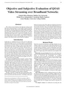
in the taxonomy. We call this pair of numbers the Relative Semantic Position (RSP) of the node. Generally, if two objects are closer to each other in terms of their semantic distance, their RSPs are also closer and vice versa. RSPs can be specified by domain experts. But to reduce the degree of user intervention, we assign a RSP to each node automatically as follows. We define the RSP of a node to consist of two numbers, denoted as (hpos, vpos), where hpos represents the horizontal position of the node in the tree and vpos represents the vertical position of the node in the tree. We use the level of the node in the tree to represent the vertical position of the node. To assign a hpos to each node, we first create a completely balanced tree by adding artificial nodes to the tree, do an in-order traversal of the balanced tree, and then remove the artificial nodes. While performing in-order traversal of the tree, we assign gradually monotonically increasing integers to the nodes of the tree as their hpos values. Therefore, the hpos value of a node is the position of the node in the balanced tree’s in-order traversal sequence. Figure 3 illustrates a tagged unbalanced tree with its RSPs assigned by this method. The benefit of this method for assigning RSPs is that the tree can be easily visualized using the RSP values in a two dimensional space. If the semantic network contains multiple trees, we can either make it a single tree by adding a root node on top of all the trees, or assign RSPs for each tree individually but with different value ranges.
Figure 4. A Rule Represented by a Line Segment in the Object Taxonomy Space Once the rules are represented using line segments, the problem of grouping association rules is converted to the problem of clustering line segments. We can use a standard clustering algorithm to cluster the line segments, and modify the distance function used in the clustering algorithm to measure the distance between two line segments. Our distance function is defined as Distance(s1 , s2 ) = 1 − cos(s1 , s2 ) + N Dist(c1 , c2 ) + N Dif f (length(s1), length(s2 )), where s1 and s2 are two line segments, cos(s1 , s2 ) takes the cosine of the angle between s1 and s2 , c1 and c2 are the center points of s1 and s2 respectively, N Dist represents normalized distance and N Dif f denotes the normalized difference, and length(x) computes the length of segment x. The SG algorithm is presented in Figure 5. It groups together rules with similar antecedents and similar consequents, and labels each group by the mean RSPs of the rules in the group, which indicate the position of the group in the semantic network. The algorithm can generate a hierarchy of clusters if a hierarchical clustering method is used for grouping line segments.
Figure 3. A Tagged Tree with RSP Values
4 A Case Study
Having assigned a RSP to each node of the taxonomy, we use RSPs to represent the objects or items in each association rule. We then calculate the average RSP of all the elements in a rule’s antecedent and the average RSP of all the elements in the rule’s consequent. The rule is then represented by two mean RSPs. Since each of the two mean RSPs corresponds to a point in a two-dimensional space, the rule can be further represented by a directed line segment (pointing from the antecedent mean to the consequent mean) in the two dimensional space. For example, consider the following rule described by the RSPs of its objects: {(2, 3), (4, 2)} → {(9, 4), (10, 3)}. We can represent the rule using the mean RSPs of its antecedent and consequent as {3, 2.5} → {(9.5, 3.5)} and further depict the rule using a directed line segment, as shown in Figure 4.
We have applied the OG and SG algorithms to group association rules discovered in a Web mining application. The data set used in the application is the Web log data produced by Livelink3, which provides automatic management and retrieval of a wide variety of information objects. From the data set, a large number of rules were generated. We first ranked the rules according to an interestingness measure [2] and then selected the top 100 rules for use in our evaluation. In the evaluation, we asked our domain expert to group the 100 rules and then compared the results from the OG and SG algorithms with the expert grouping. Our domain expert 3 Livelink is a commercial product of Open Text Corporation (http://www.opentext.com).
3
Algorithm: Subjective Grouping Input: a tagged tree or forest; a set of mined association rules R; Output: a set of grouped association rules Begin
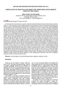
run the SG algorithm, we first tagged the trees with our automatic tagging method. We then used a hierarchical agglomerative clustering algorithm to cluster the line segments within the SG program. The program generates a dendrogram that shows the levels of nested merging. When we evaluate the performance, we cut the dendrogram at the level where there are 15 clusters, and based on these clusters we calculate the grouping accuracy. Due to the use of hierarchical clustering, the result of grouping is also a tree of clusters. The number of levels shown in Table 2 for the SG run is the level of the tree produced on top of the 15 clusters. In general, the program can do k-way clustering. Here we set k to be 15, which is the actual number of groups produced by the expert. From Table 2 we can see that the SG algorithm produces more accurate results than the OG algorithm.
1. For each rule in R Begin 2.
Replace each item in the rule with its RSP;
3.
Compute the mean of RSPs of all the items in the antecedent of the rule and the mean of RSPs of all the items in the consequent;
4.
Add the two means and the rule id as a record in table T
5. End 6. Call a clustering algorithm to group the line segments (represented by the two means) in T , using our distance function; 7. Label each group with the mean of RSPs in the antecedents and the mean of RSPs in the consequents of the rules in the group; 8. Return the grouped association rules; End
5 Conclusions
Figure 5. The Subjective Grouping Algorithm Group size Num. of groups
1 4
2 4
3 1
4 1
5 2
20 1
25 1
We have presented two new algorithms for grouping a large number of (interesting) association rules. We also presented a case study in which we applied the two algorithms to group a set of interesting association rules discovered from the Livelink log data. Our experiment shows that both methods are effective and produce good grouping result with respect to the expert grouping result.
26 1
Table 1. Group Size Distribution from Experts groups the 100 rules into 15 groups. The distribution of the group size is shown in Table 1. The results of OG and SG are shown in Table 2. There are two runs of the OG algorithm (OG-1 and OG-2), using two different thresholds (i.e., the maximum numbers of the rules in a cluster). Each run of OG produces a tree of clusters. The table shows the number of levels of the cluster tree, the number of clusters at the lowest non-leaf level (shown in the table as No. of clusters), the number of lowest non-leaf level clusters that are completely the same as a cluster from the expert (No. of compl. cor. clusters) and the grouping accuracy. The grouping accuracy is calculated as follows. For each pair of rules, we know whether they should belong to the same group based on the grouping result from the domain expert. If two rules that should belong to the same group are clustered into the same group or if two rules that should not belong to the same group are clustered into different groups, we call it a “match”; otherwise, it is a mis-match. The grouping accuN umber of matches racy is defined as accuracy = T otal number of rule pairs .
Acknowledgment We would like to thank Open Text Corporation and CITO for supporting this research, and Mr. Miao Wen for his help in implementing the algorithms presented in the paper.
References [1] Adomavicius, G. and Tuzhilin, A. ”Expert-driven validation of rule-based user models in personalization applications”, Data Mining and Knowledge Discovery, vol.5, nos.1/2, January/April 2001. [2] Huang, X., An, A., Cercone, N and Promhouse, G. ”Discovery of Interesting Association Rules from Livelink Web Log data”, Proc. of the IEEE Int. Conf. on Data Mining (ICDM’02), Maebashi City, Japan, 2002. [3] Lent, B., Swami, A.N., and Widom, J. ”Clustering Association Rules”, Proc. of ICDE, 1997.
The information objects in the Livelink environment are organized into a structure that contains over 2000 trees. To Run OG-1 OG-2 SG
Threshold 26 20 15
No. of levels 3 4 9
No. of clusters 11 13 15
No. of compl. cor. clusters 6 4 12
[4] Sahar, S., ”Interestingness via What is not Interesting”, Proceedings of KDD’99, 1999, pp.332-336. [5] Toivonen, H., Klemettinen, M., Ronkainen, P., Hatonen, K. and Mannila, H. ”Pruning and grouping discovered association rules”, Proc. of KDD’95.
Accuracy 81.2% 71.5% 93.7%
[6] Wang, K., Tay, S.H.W. and Liu, B. ”Interestingnessbased interval merger for numeric association rules”, Proc. of KDD’98.
Table 2. Results of the OG and SG Algorithm 4