Objective Bayesian Snalysis for the Complementary ...

International Journal of Statistics and Probability; Vol. 6, No. 2; March 2017 ISSN 1927-7032 E-ISSN 1927-7040 Published by Canadian Center of Science and Education

Objective Bayesian Snalysis for the Complementary Exponential Geometric Model Applied to Cancer Data Daniele C. T. Granzotto1 , Vera Tomazella2 & Francisco Louzada3 1

Departamento de Estat´ıstica, Universidade Estadual de Maring´a, Av. Colombo, 5.790, Maring´a-PR, 87020-900, Brazil

2

Departamento de Estat´ıstica, Universidade Federal de S˜ao Carlos, Via Washington Lu´ıs, km 235, Caixa Postal 676, 13565-905, S o Carlos, SP, Brazil 3

Instituto de Ciˆencias Matemticas e da Computac¸a˜ o, Universidade de S˜ao Paulo, Caixa Postal 668, So Carlos, SP, 13566590, Brazil Correspondence: Daniele C. T. Granzotto, Departamento de Estat´ıstica, Universidade Estadual de Maring´a, Av. Colombo, 5.790, Maring´a-PR, 87020-900, Brazil. E-mail:[email protected] Received: December 9, 2016 doi:10.5539/ijsp.v6n2p122

Accepted: February 15, 2017

Online Published: February 23, 2017

URL: https://doi.org/10.5539/ijsp.v6n2p122

Abstract In this paper we provide a reference Bayesian framework to a new two-parameter lifetime distribution with increasing failure rate, the complementary exponential geometric (CEG). To this end, we presented some of the main properties of this model and its characteristics related to the reliability analysis. A simulation study is performed to analyse the frequentist properties of credible intervals from the reference posterior distribution among of the standard error and mean square error (MSE) of estimations. The presented methodology is illustrated by the use of a real data set which presents the study of time until the cure of cervix lesions, that are precursors cancer lesions in the cervix. According to to INCA (Cancer National Institute), cervical cancer stands as the fourth cause of death among women in Brazil. Together with breast cancer, it is one of the most common malignancy affecting women worldwide. For this reason, patients must be carefully evaluated for metastatic disease. These data were collected in the Woman Clinic which is sited in Maring´a city (Paran´a State, Brazil). Keywords: CEG distribution, bayesian analysis, objective prior, survival analysis 1. Introdution Cervical intraepithelial neoplasia (CIN), also known as cervical dysplasia and cervical interstitial neoplasia, is the potentially premalignant transformation and abnormal growth (dysplasia) of squamous cells on the surface of the cervix. Most cases of CIN remain stable, or are eliminated by the host’s immune system without intervention. However a small percentage of cases progress to become cervical cancer, usually cervical squamous cell carcinoma (SCC), if left untreated. The major cause of CIN is chronic infection of the cervix with the sexually transmitted human papillomavirus (HPV), especially the high-risk HPV types 16 or 18. Over 100 types of HPV have been identified. About a dozen of these types appear to cause cervical dysplasia and may lead to the development of cervical cancer. The estimated annual incidence in the United States of CIN among women who undergo cervical cancer screening is 4 percent for CIN 1 and 5 percent for CIN 2,3. High grade lesions are typically diagnosed in women 25 to 35 years of age, while invasive cancer is more commonly diagnosed after the age of 40, typically 8 to 13 years after a diagnosis of a high grade lesion. It is estimated that about 500,000 new cases are reported every year, with approximately 230,000 deaths worldwide. In Brazil, the crude incidence rates per 100,000 women, estimated for the year 2012, were 17 for the country and 14 for the Rio Grande do Norte State. The incidence of the disease starts from the age of 20 and the risk gradually increases with age, reaching its peak generally at age 50 to 60, (Limaetal, 2013; Ferenczy, 1982). In Brazil, the coverage of the cytopathology exam has not still reached the desired indices. It is estimated that approximately 40% of Brazilian women have never undergone the procedure. This is due to several factors, including the difficulty of access to health services, poor knowledge about the Pap smear, and the lack of awareness of the benefits that this exam brings to womens health (for more informations see INCA website). The recognition of the central role of HPV in the etiology of cervical cancer has dramatically changed the vision of how to prevent this cancer. Among the strategies, introduction of HPV testing for primary screening or as an adjunct test and the introduction of HPV vaccines to prevent HPV infection are being evaluated in different settings around the world. Indeed, these advances are available in many countries that have approved the introduction of the HPV vaccine. However, gaps in knowledge about the causal role of HPV in cervical cancer and the benefits of preventing HPV infection may hamper the successful introduction of the technologies. The greater the womens knowledge of HPV and its role in the development of cervical cancer, the greater will be the adherence to preventive measures.

122

http://ijsp.ccsenet.org

International Journal of Statistics and Probability

Vol. 6, No. 2; 2017

The presented methodology in this paper is applied to a real study involving patients treated in the Woman Clinic sited in Maring´a city, Paran´a State, Brazil. The data consist of the time until the cure of CIN (in months) in 363 women followed up from years 2,000 to 2,006. For all patients was observed the maximum time that the initial lesions took to be considered totally cure (after specific diagnostics). We consider a new two-parameters lifetime distribution with increasing failure rate, the complementary exponential geometric distribution proposed by (Louzada, et al., 2011). which is complementary to the exponential geometric model proposed by Adamidis & Loukas (1998). The new distribution arises on a latent complementary risks scenarios, where the lifetime associated with a particular risk is not observable, rather we observe only the maximum lifetime value among all risks. This distribution is based on a generalization of the the exponential distribution, which is a widely used lifetime distribution for modeling many problems in lifetime testing and reliability study. According to Bernardo (Bernardo, 1979), in the quest for objective posterior distributions, several requirements have emerged which may reasonably be requested as necessary properties of any proposed solution: generality such procedure should be completely general; invariance(Jeffreys, 1946; Datta Ghosh, 1995; Datta Ghosh, 1996); present consistent marginalization; and the properties under repeated sampling of the posterior distribution must be consistent with the model (Neyman Scott, 1948; Lane Sudderth, 1984). Under these cited assumptions, Bernardo (Bernardo, 1979) introduced the reference analysis which was further developed by Berger and Bernardo (Berger Bernardo, 1992a) and Berger and Bernardo (Berger Bernardo, 1992b). The technique, according to those authors, appears to be the only available method to derive objective posterior distributions which satisfy all these desiderata and even for moderate sample sizes, the information provided by the data should dominate the prior information because of the vague nature of the prior knowledge. Alternative to this reference prior, the Jeffreys prior is widely used in Bayesian with an important characteristic that it is invariant under injective transformations (Paulino, et al., 2003). Despite the property of invariance, the posterior distribution by using Jeffreys prior may be improper (unlike by using reference prior) and lead to a uninformative distribution. Also, the use of the Jeffreys rule in the multiparametric case is often inadequate. The assumption of a prior independence between parameters of different natures, and the separate use of Jeffreys rule for specification of marginal distributions may give different results than obtained by the Jeffreys principle (Berger, 1985). So, in this paper the parameter estimation will be considered from the reference Bayesian perspective for the parameters of the the complementary exponential geometric (CEG) distribution (the MLEs of the CEG model in a classical context can be seem in (Louzada, et al., 2011)). The paper is organized as follows. Section 2, we presented a briefly introduction to a model CEG with some particularities and an overview of reference analysis with emphasis on the case of two parameters. In Section 3, the inference for the CEG model is presented by using the reference prior built. After presenting the model and inference aspects, a simulation study was made and it can be seem in Section 4. Finally, in Sections 5 and 6, respectively, we can see the usefulness of the CEG model in a Bayesian context by studying the time until the cure of precursors cancer cervix lesions and some conclusions. 2. Background 2.1 The CEG Model Proposed by (Louzada, et al., 2011), the CEG model was formulated to describe lifetime with increasing failure rate. According to the authors, this is complementary to the exponential geometric model proposed by Adamidis and Loukas (Adamidis Loukas, 1998) and arises on a latent complementary risks scenario, in which the lifetime associated with a particular risk is not observable. Instead, we observe only the maximum lifetime value among all risks. For more details on latent risk problem, interested readers can refer to Basu and Klein (Basu Klein, 1982) and Louzada-Neto (Louzada-Neto, 1999). Let M be a random variable denoting the number of failure causes, m = 1, 2, . . ., and considering M with geometrical distribution of probability given by P(M = m) = θ(1 − θ)m−1 , (1) where 0 < θ < 1 and M = 1, 2, . . .. Let us also consider ti , i = 1, 2, 3, . . ., realizations of a random variable denoting the failure time, i.e., the time-to-event due to the ith complementary risk, with T i having an exponential distribution with probability index λ, given by f (ti |λ) = λ exp{−λti }.

(2)

In the latent complementary risk scenario, the number of causes M and the lifetime ti associated with a particular cause are 123

http://ijsp.ccsenet.org

International Journal of Statistics and Probability

Vol. 6, No. 2; 2017

not observable (latent variables), and only the maximum lifetime Y among all is usually observed. So, we only observed the random variables given by Y = max(t1 , t2 , . . . , t M ).

(3)

By considering those descriptions, the model CEG was built and the Proposition 2.1 follows. Proposition. Let Y be a nonnegative random variable denoting the lifetime of an individual in some population. The random variable y is distributed according to a CEG distribution, with parameters λ ∈ Λ and θ ∈ Θ, Λ = {λ; λ ∈ (0, +∞)}, Θ = {θ; θ ∈ (0, 1)}, if its probability density function (pdf) and cumulative distribution function are given, respectively, by λθe−λy f (y|θ, λ) = ( ) , e−λy (1 − θ) + θ 2 and F (y|θ, λ) =

( ) θ 1 − e−λy e−λy (1 − θ) + θ

(4)

.

(5)

Proof. The build of CEG model and some specific properties can be find in Louzada et al. (Louzada, et al., 2011).

1.0 0.8 0.6

θ = 0.001 θ = 0.01 θ = 0.1 θ = 0.9 θ = 0.99

0.2 0.0

0.0

0.2

0.4

Density

Cumulative

0.6

0.8

θ = 0.001 θ = 0.01 θ = 0.1 θ = 0.9 θ = 0.99

0.4

1.0

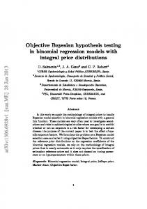
In order to show the behaviour of the probability density and cumulative function are shown, respectively, in left and right panels of the Figure 1.

0

5

10

15

0

y

5

10

15

y

Figure 1. pdf and cdf of the CEG distribution with parameter λ = 2 fixed. In reliability analysis, we have interest in two important characteristic of a random variable Y that represents the lifetime, namely, the reliability function R(y|θ, λ), which is the probability of an item not failing prior to some time y, is defined by R(y|θ, λ) = 1 − F(y|θ, λ); and the hazard function, which can be loosely interpreted as the conditional probability of failure, given it has survived to the time y(Lawless, 2003). In what follows, we exhibit the equations of reliability and hazard functions; else, in Figure 2 we show the behaviour of the reliability and hazard functions for some specifics values of parameter θ and λ = 2 fixed. Let Y be a nonnegative random variable denoting the lifetime of an individual in some population. The reliability function R(y|θ, λ) is written as e−λy , (6) − θ) + θ where λ ∈ Λ and θ ∈ Θ are the scale and shape parameters. The hazard, h(y|θ, λ), and cumulative hazard rate, H(y|θ, λ) functions are given by R (y|θ, λ) =

h (y|θ, λ) =

e−λy (1

θλ e−λy (1 − θ) + θ 124

(7)

θ = 0.001 θ = 0.01 θ = 0.1 θ = 0.9 θ = 0.99

θ = 0.001 θ = 0.01 θ = 0.1 θ = 0.9 θ = 0.99

0.0

0.0

0.2

0.5

0.4

1.0

Hazard

Survival

0.6

1.5

0.8

Vol. 6, No. 2; 2017

2.0

International Journal of Statistics and Probability

1.0

http://ijsp.ccsenet.org

0

5

10

15

0

5

y

10

15

y

Figure 2. Survival and hazard of the CEG distribution with parameter λ = 2 fixed.

and [ ] H (y|θ, λ) = ln e−λy (1 − θ) + θ − ln θ − ln(1 − e−λy ),

(8)

λ ∈ Λ and θ ∈ Θ. 2.2 Reference Analysis In this section we present the declared objective of reference Bayesian analysis introduced by (Bernardo,1979) and further developed by (Berger Bernardo, 1992a) and(Berger Bernardo, 1992b) is to specify a prior distribution such that, even for moderate sample sizes, the information provided by the data should dominate the prior information because of the “vague” nature of the prior knowledge. An important feature in the Berger-Bernardo approach to construct a non-informative prior is the different treatment for interest and nuisance parameters. When there are nuisance parameters (typical case in this paper), one must establish an ordered parametrization with the parameter of interest singled out and then follow the procedure below. Proposition. Let p (x|θ, λ) , (θ, λ) ∈ Θ × Λ(θ) ⊆ R × R be a probability model with two real-valued parameters θ and λ, where θ is the quantity of interest. Let I(θ, λ) the corresponding 2x2 Fisher’s matrix in terms of θ and λ, and let V(θ, λ) = I −1 (θ, λ). Suppose that the joint posterior distribution of (θ, λ) is asymptotically normal with covariance matrix ˆ λ), ˆ where θˆ and λˆ are the corresponding consistent estimators of θ and λ. It follows that: V(θ, (i) the conditional reference prior of λ given θ is π (λ | θ) ∝ [I22 (θ, λ)]1/2 , (ii) if π (λ|θ) is not proper, a compact approximation {Λi (θ) , given θ is

i = 1, 2...} to Λ (θ) is required, and the reference prior of λ

[I22 (θ, λ)]1/2

πi (λ|θ) = ∫

λ ∈ Λ (θ)

[I22 (θ, λ)]1/2 dλ

,

λ ∈ Λi (θ)

Λi (θ)

(iii) the sequence of priors can be obtained as     ∫     [ ]     1/2 (λ|θ) (θ, , π log v λ) dλ πi (θ) ∝ exp   i   11       Λi (θ)

125

http://ijsp.ccsenet.org

International Journal of Statistics and Probability

Vol. 6, No. 2; 2017

−1 (θ, λ) = Iθ (ϕ, λ) =I11 − I12 I22 where v1/2 I21 11

(iv) the reference posterior distribution of θ given data {y1 , ..., yn } is   ∫     π(θ|y1 , ..., yn ) ∝ π(θ)     

  n          ∏   (y (λ|θ) p |θ, λ) π dλ .    l         l=1

Λ(θ)

Proof. See a heuristic justification in Bernardo (2005). 1/2 (θ, λ) and I22 Corollary. If the nuisance parameter space Λ (θ) = Λ is independent of θ, and the functions v−1/2 (θ, λ) 11 factorize in the form {I22 (θ, λ)}1/2 = f2 (θ) g2 (λ) . {v11 (θ, λ)}−1/2 = f1 (θ) g1 (λ) ,

Then π(θ) ∝ f1 (θ) , π (λ|θ) ∝ g2 (λ) . Thus, the reference prior relative the ordered parametrization (θ, λ) is given by π (λ, θ) = f1 (θ) g2 (λ) and there is no need for compact approximation, even if the conditional reference prior π (λ|θ) is not proper. Proof. See proof of Theorem 12 in Bernardo (2005). 3. Reference Prior for the CEG Model According to Bernardo (2005), let yk = (y1 , . . . , yk ) k-independent replications of the CEG model and consider h(θ, λ) = 1 a positive function. Then, q(θ, λ, y1 , . . . , yk ) ∝ L(θ, λ)h(θ, λ) is an asymptotic approximation of posterior distribution. Under certain regularity conditions whereas there is a maxˆ k ), λ(y ˆ k )) we have that the posterior density q(θ, λ, y1 , . . . , yk ) is approximately normal imum likelihood estimator (θ(y k-dimensional, i.e, ( ) ˆ λ), ˆ nI(θ, ˆ λ) ˆ , q(θ, λ, y1 , . . . , yk ) ∼ Nk (θ,

(9)

ˆ λ) ˆ is the Fisher information matrix. where I(θ, Considering that the posterior distribution is assymptotically normal, then the reference prior only depends on Fisher information matrix. Here we derive the reference prior considering the approach of one nuisance parameter described above. Then, the likelihood and log-likelihood functions of (θ, λ) based on the observed sample of size n, y = y1 , y2 , . . . , yn , from the CEG distribution (4) are given, respectively, by ∑ λn θn exp(−λ ni=1 yi ) L (θ, λ|y1 , . . . , yn ) = ∏n [ (10) ] −λyi (1 − θ) + θ 2 i=1 e and l (θ, λ|y1 , . . . , yn ) = n log(λθ) − λ

n ∑ i=1

yi − 2

n ∑

] [ log e−λyi (1 − θ) + θ .

(11)

i=1

In order to find the Fisher information matrix, the first-order derivates of the log-likelihood function (11) for a single observation are given by [ ] 1 − e−λy ∂l (θ, λ|y1 , . . . , yn ) 1 = − 2 −λy (12) ∂θ θ e (1 − θ) + θ and

[ ] ∂l (θ, λ|y1 , . . . , yn ) 1 (1 − θ)ye−λy = − y + 2 −λy . ∂λ λ e (1 − θ) + θ 126

(13)

http://ijsp.ccsenet.org

International Journal of Statistics and Probability

Vol. 6, No. 2; 2017

The second-order derivates of the log-likelihood function (11) are given by ∂2 l (θ, λ; y) ∂θ2 ∂2 l (θ, λ; y) ∂λ2 2 ∂ l (θ, λ; y) ∂λ∂θ

[ ]2 1 eλy − 1 + 2 , 1 + θ(eλy − 1) θ2 ) ( 1 + θ θ − 2 + θe2λy − 2(1 − θ)(1 + λ2 y2 )eλy

= − =

(1 + θ(eλy − 1))2

=

(

2yeλy 1 + θ(eλy − 1)

,

)2 .

Finally, the Fisher information matrix for model CEG is given by   I(θ, λ) = n 

1 3θ2 (θ−1)θ−log(θ) 3λθ(θ−1)2

(θ−1)θ−log(θ) 3λθ(θ−1)2 −(1+θ)+2Li2 (β) 3λ2 (1−θ)

  

∑ where Li2 (·) represents the polylogarithm function given by Li2 (β) = ∞ k=1 Information matrix for a single observation, presented in (14), is given by   V(θ, λ) = 

3(1−θ)(1+θ−2Li2 (β)) ζ(θ) 3(1−θ)2 θλ(θ(θ−1)−log θ) ζ(θ)

(14) (−β)k k2

3(1−θ)4 λ2 ζ(θ)

and β =

1−θ θ .

The inverse of Fisher

   , 

(15)

where ζ(θ) = (1 − θ)2 + 2(1 − θ)θ + log(θ)2 + 2(θ − 1)3 Li2 (β). Form Collorary 2.2 and the Equation (14), the join reference prior density of CEG model, with two real-valued parameters θ and λ, π (θ, λ) , (θ, λ) ∈ Θ × Λ(θ) ⊆ R × R is given by π(θ, λ) ∝

π(θ) , λ

(16)

where π(θ) ∝

√

[ ]−1/2 φ(θ) −3(θ − 1)3 θ2 (1 + θ − 2Li2 (β)) ,

and φ(θ) = (θ − 1)2 − 2(θ − 1)θ log(θ) + log(θ)2 + 2(θ − 1)3 Li2 (β), where Li2 (β) is the polylogarithm function defined as Li2 (β) =

∑∞

(−β)k k2

k=1

and β =

1−θ θ .

Combining the likelihood function in (11) and the prior (16), the joint posterior distribution for θ, λ is given by, ∑n

θn λn−1 e−λ i=1 yi π(θ, λ|y1 , . . . , yn ) ∝ ∏n [ ] π(θ). −λyi (1 − θ) + θ) 2 i=1 e

(17)

In Appendix A we show that the join posterior distribution is proper. 4. Simulation Study Louzada et al. (2011) performed a misspecification simulation study for the CEG model, in order to assess the extent of misspecification errors when testing the exponential geometric distribution against the complementary one in the presence of different sample size and censoring percentage. The authors discovered that it is usually possible to discriminate between the distributions even for small samples in the presence of heavy censoring by using the MLEs in a classical inference context (for sample sizes more than 50). Aiming to examine the finite sample properties of the MLEs, this section presents the results of a Monte Carlo experiment in a Bayesian context. For that, we use 1, 000 Monte Carlo replications in all presented results. The sample sizes n range from 50 to 1, 000, generated according to a CEG distribution for each combination of the parameter value θ = (0.1; 0.3; 0.5) and λ = 2 fixed. The lifetime times of this model were generated by considering the inverse transformation of the cumulative function (Ross, 2009), as follow. 127

http://ijsp.ccsenet.org

International Journal of Statistics and Probability

Vol. 6, No. 2; 2017

Proposition. Let F(y|θ, λ), y ∈ (0, +∞), denoted a cumulative distributions function of a CGE model. Define Y = F −1 (U), where U has a continuous uniform distribution over the interval (0, 1). Then Y is distributed as F, that is, P(Y ≤ x) = F(y), y ∈ (0, +∞) and the lifetimes are generate as ( ) 1 θ(1 − u) −1 Y = F (U) = − ln . (18) λ θ(1 − u) + u The samples are subsequently obtained by the Metropolis-Hastings technique through the MCMC implemented in software SAS 9.3 - Statistical Analysis System, by using the procedure MCMC with a single chain of the dimension 50, 000. A burn-in of 10, 000 was adopted in order to eliminate the effect of the initial values, resulting a sample size 40, 000. The convergence of the chain was checked by the criterion proposed by Geweke (1992) for each set of simulated data and an average of the estimates of the parameters and standard deviation (SD), the mean square error and the coverage probability of the 95% posterior credible intervals was obtained by using the reference distribution prior. The coverage probability of the posterior credible interval was proposed, in instead of the confidence interval, once we are interested in study and apply this model in a Bayesian context. Table 1 show the MLEs by using the reference prior presented in Section 3. We can observed that the variances of the MLEs and their mean square error (MSE) become smaller when the sample size increases. Also, the coverage probability of a 95% two sided credibility intervals, for the model parameters, are observed to be close to the nominal coverage for large sample sizes, though the usually differ from the nominal coverage probability less than 2% for moderate sample sizes (more than 100). Note that, the simulation was proposed to check the behaviour of the MLEs for finite sample sizes. Although the bias is large and the coverage probability of the credibility intervals for the model parameters is far from the nominal value, for samples with size less than 100, we intend to applie the same inference method in a real study related to the cervical intraepithelial neoplasia with sample size more than 300 patients. When we considere that specific sample size, n=300, we observe that the bias is undercontrol and the coverage probability is really close to the proposed nominal value. Table 1. Mean of parameters estimated and SD, the mean square error (MSE) and coverage probability for each combination of sample size and generated parameters, by using the reference prior 2*Generated n 50

100

150

300

500

1, 000

θ 0.1 0.3 0.5 0.1 0.3 0.5 0.1 0.3 0.5 0.1 0.3 0.5 0.1 0.3 0.5 0.1 0.3 0.5

2*Simulated θˆ 0.325 0.571 0.600 0.127 0.369 0.544 0.117 0.344 0.542 0.108 0.322 0.530 0.105 0.313 0.519 0.1022 0.306 0.5087

λˆ 1.134 1.047 1.575 1.951 1.928 2.017 1.972 1.970 2.006 1.987 1.988 1.996 1.992 1.993 1.997 1.997 1.998 2.000

ˆ SD(θ) 0.089 0.154 0.177 0.047 0.123 0.154 0.035 0.096 0.135 0.022 0.063 0.102 0.017 0.047 0.079 0.011 0.033 0.054

ˆ SD(λ) 0.402 0.455 0.484 0.234 0.297 0.307 0.187 0.232 0.254 0.132 0.164 0.186 0.102 0.127 0.145 0.072 0.090 0.102

128

Mean Squared Error MSEθ MSEλ 0.058 0.912 0.097 1.115 0.041 0.415 0.003 0.057 0.020 0.094 0.026 0.095 0.001 0.036 0.011 0.055 0.020 0.065 0.001 0.018 0.004 0.027 0.011 0.035 0.000 0.010 0.002 0.016 0.007 0.021 0.000 0.005 0.001 0.008 0.003 0.011

Coverage Probability CPθ CPλ 0.660 0.654 0.697 0.684 0.910 0.872 0.930 0.942 0.937 0.939 0.968 0.965 0.934 0.935 0.933 0.928 0.946 0.945 0.935 0.956 0.941 0.959 0.946 0.955 0.946 0.949 0.947 0.952 0.949 0.951 0.948 0.950 0.952 0.947 0.948 0.946

http://ijsp.ccsenet.org

International Journal of Statistics and Probability

Vol. 6, No. 2; 2017

5. Cervical Intraepithelial Neoplasia Data Recall the CIN data presented in the introductory section. In this section we illustrate the usefulness of the CEG distribution by using the reference prior on modeling such a real data set. Firstly, a brief descriptive analysis was made. The minimum observed time was 1 month and the maximum observed one was 47 months, approximately four years. The mean time for the cure is 6.4 months with 5.099 SD. The left panel of the Figure 3 shows the TTT plot (Barlow Campo, 1975), in order to verify the possible shape for the hazard function. If the TTT plot is concave, it indicates increase hazard, which can accommodate by a CEG distribution.

0.30

Empirical CEG Exponential

0.25 0.20

Hazard 0.0

0.0

0.10

0.2

0.2

0.15

0.4

0.4

f

Survival

0.6

0.6

0.8

0.8

1.0

1.0

TTT plot

0.0

0.2

0.4

0.6

0.8

1.0

0

10

r/n

20

30

40

0

10

20

t

30

40

t

Figure 3. Left panel: TTT plot. Middle panel: estimated survival curves according to the CEG and Exponential distribution fittings over imposed on the Kaplan-Meier empirical curve. Right panel: estimated hazard function according the CEG distribution. After initial analysis, the CEG model was fitted the data. As the exponential model is a particular case of CEG model when θ = 1, this model was fitted too. The posterior samples (for both models), were generated by the Metropolis-Hastings technique, similar to the simulation study. An single chain of the dimension 100, 000 was considered for each parameter, discarting the first 20, 000 iterations to eliminate the effect of the initial values, and to avoid correlation problems, a lag with size 20 was used, resulting in a final sample 4, 000. Table 2 shows the posterior summaries for the parameters and the 95% credible intervals considering the reference. Table 2. Posterior model summary of CEG model by considering the reference prior 2*Models 2*CEG Exponential

2*Parameters θ λ λ

2*Mean 0.232 0.310 0.154

2*SD 0.041 0.023 0.008

25% 0.202 0.295 0.148

Percentiles 50% 75% 0.228 0.257 0.310 0.310 0.154 0.160

2*IC (95%) 0.159 0.263 0.138

0.318 0.351 0.171

The convergence of the chain was verified by Geweke criterion (Geweke, 1992) which demonstrate that these criteria are satisfied for both models, as follows in Table 3. Also, the acceptance rates were obtained too. Table 3. Geweke criteria and acceptance rate Model 2*CEG Exponential

Parameter θ λ λ

z −0.8442 0.0037 0.3976

p-value 0.3986 0.9971 0.6909

Acceptance Rate 2*0.3289 0.3692

In order to compare these models, the deviance information criterion (DIC), which is a hierarchical modelling generalization of the AIC (Akaike information criterion) and BIC (Bayesian information criterion, also known as the Schwarz criterion), was obtained. This criteria is particularly useful in Bayesian model selection problems where the posterior distributions of the models have been obtained by Markov chain Monte Carlo (MCMC) simulation which is our case. The idea is that models with smaller DIC should be preferred to models with larger DIC which is the case of CEG model with DIC = 2, 006.797 against 2, 075.498 for the exponential model. 129

http://ijsp.ccsenet.org

International Journal of Statistics and Probability

Vol. 6, No. 2; 2017

In addition to this criterion, it is possible to visually distinguish the model that best fits this data set. The middle panel of the Figure 3 shows the survival curves estimated empirically and by the model CEG and exponential. Clearly, we can see that the estimated survival curve for the model CEG is closer to a empirical curve than the model exponential which suggest that CEG model fits better in this case. Furthermore, in right panel of the Figure 3 we can see the increasing behavior of the estimated hazard curves for models CEG.

0.50 0.45 λ

0.40

6

Density

0.25

0

0

2

0.30

1

4

0.35

2

Density

3

8

4

10

5

12

0.55

Figure 4 shows the marginal posterior density for unknown quantities θ and λ, left and middle panels, respectively. Also, right panel shows the scatterplot to analyze the convergence of the parameters by considering two distinct initial values.

1.4

1.6

1.8

2.0

2.2

2.4

2.6

0.15

θ

0.20

0.25

0.30 λ

0.35

0.40

0.05

0.10

0.15

0.20

0.25

0.30

0.35

θ

Figure 4. Marginal posteriors densities and scatterplot to analyze the convergence of the parameters by considering two distinct initial values ˆ λ(1 ˆ − θ)] ˆ = 6.14 Considering the CEG distribution fitting, the expected cure time for cervix lesions is E(T ) = − ln(θ)/[ months. The 95% credible interval for expected cure time ranges from 4.79 to 8.30 months. Moreover, the modal value for the time until the cure is given by M(Y) = λ1 ln 1−θ θ = 3.87 months with a 95% credible interval ranging from 2.17 to 6.32 months. 6. Concluding Remarks In this paper we presented the reference Bayesian inferential procedure for the CEG distribution. The reference Bayesian analysis is an alternative to the Jeffreys prior. In contrast to the Jeffreys, as we show that the prior is permissible then the reference prior leads to a proper posterior distribution. After some discussion about the reference prior, we made a simulation study where we can observe the adequacy of the proposed inferential method by using different sample sizes. The simulated results show better frequentist properties for samples sizes of above 100. In order to illustrate the usefulness and effectiveness of the Bayesian CEG model, one real data set was considered which studies the time to cure of precursors lesions of cervical cancer. The use of complementary model was extremely important in this case because it did not know the times in which each lesions were cured but the final time (in this case the maximum time), in which all had been eliminated. If we chose on an usual model for survival analysis, this important peculiarity has not been observed. 7. Proof that the Posterior Distribution is Proper The join posterior distribution is given by

π(θ, λ|y1 , . . . , yn )

∝

∑ θn λn−1 exp(−λ ni=1 yi ) ∏n [ ]2 × i=1 exp(−λyi )(1 − θ) + θ ]1/2 [ (θ − 1)2 − 2(θ − 1)θ log θ + (log θ)2 + 2(θ − 1)3 Li (β) . 3(θ − 1)3 θ2 [(1 + θ) − 2Li (β)]

Note that 130

http://ijsp.ccsenet.org

International Journal of Statistics and Probability

Li (β) =

∞ ∑ (θ − 1)k

k2

k=1

= (θ − 1) +

(θ − 1)2 (θ − 1)3 (θ − 1)4 + + + ... 22 32 42

< =

(θ − 1)2 (θ − 1)4 (θ − 1)6 ++ + + ... 2 2 42 62 (θ − 1)2 + (θ − 1)4 + (θ − 1)6 + (θ − 1)8 + . . . [ ] (θ − 1)2 1 + (θ − 1)2 + (θ − 1)4 + (θ − 1)6 + . . .

=

(θ − 1)2