Observability in Inertial Parameter Identification - arXiv

1

Observability in Inertial Parameter Identification

arXiv:1711.03896v1 [cs.RO] 10 Nov 2017

Patrick M. Wensing, G¨unter Niemeyer, Jean-Jacques E. Slotine

Abstract—We present an algorithm to characterize the space of identifiable inertial parameters in system identification of an articulated robot. This problem has been considered in the literature for decades; however, existing methods suffer from common drawbacks. Methods either rely on symbolic techniques that do not scale, or rely on numerical techniques that are sensitive to the choice of an input motion. The contribution of this work is to propose a recursive algorithm for this problem that requires only the structural parameters of a mechanism as its input. This Recursive Parameter Nullspace Algorithm (RPNA) can be applied to general open-chain kinematic trees, and does not rely on symbolic techniques. Drawing on the exponential parameterization of rigid-body kinematics, classical linear controllability and observability results can be directly applied to inertial parameter identifiability. The high-level operation of the RPNA is based on a key observation – undetectable changes in inertial parameters can be interpreted as sequences of inertial transfers across the joints. This observation can be applied recursively, and lends an overall complexity of O(N ) to determine the minimal parameters for a system of N bodies. M ATLAB source code for the new algorithm is provided. Index Terms—Dynamics, Calibration and Identification

I. I NTRODUCTION A classic problem in robotics is the identification of inertial parameters (mass, center of mass, and inertia) for each link of a mechanism. This problem has received attention through multiple decades, with original work for identification of manipulators [1], [2], [3] seeing extensions to identification of mobile robots and humans in more recent applications [4], [5], [6], [7], [8]. Across domains, an enabling property is that the inverse dynamics of a rigid-body system are linear in its inertial parameters. This property has motivated wide use of simple least-squares methods to identify parameters from the measurement of joint torques and/or external forces, and has likewise enabled adaptive control [9], [10]. System identification methods have become increasingly important due to the growth of model-based control in emerging applications of legged robotics [11], [12], [13]. Advances in whole-body control [14], [15], [16], [17], [18] have enabled modern platforms to reason through the interplay between their motion and required interactions with the environment. Careful consideration is needed to respect unidirectional and frictional limitations on these interaction forces, and this consideration can only be accomplished by reasoning over dynamic models. Control in periods of underactuation is further sensitive to model details, in part, motivating the prevalence of flat-footed gaits in many platforms. These considerations jointly motivate the desire for mature sets of tools for the community to quickly build accurate models from data. A. Previous Work to Understand Unidentifiable Parameters A feature of the parameter identification problem is that not all inertial parameters are observable from measurement of

the external forces and joint torques. That is, certain numeric changes in inertial parameters of a mechanism cause no change to its dynamics. Within identification, this general phenomena is known as a lack of structural identifiability [19] and has been studied extensively within the robotics identification literature [1], [2], [20], [21], [22], [23], [24], [25], [23], [26], [27]. Since the dynamics of a mechanism may be derived from its kinetic and potential energies, methods often equivalently consider identifiability of energetic quantities. Methods to determine unobservable inertial parameters are split between symbolic and numeric approaches, with both introduced in the seminal work of Atkeson, An, and Hollerbach [1]. Symbolic manipulation of kinetic and potential energies was originally developed to decrease computation in the Recursive Newton-Euler algorithm by reducing the number of inertial parameters in the algorithm [20]. Gautier and Khalil refined initial results to include more general cases through a series of papers [21], [22], [23], [24], noting applicability to system identification. Similar symbolic techniques led to many helpful rules of thumb to determine minimal parameters in special cases such as revolute manipulators with parallel and perpendicular joints [25], [26]. The complexity of symbolic manipulations, and limitation to special cases, motivated the development of more scalable and general methods. By sampling the so-called inverse dynamics regressor at a number of points, unidentifiable parameters for the input data can be deduced via SVD or QR decompositions [23], [27], [28]. This can be done without costly symbolic regroupings of parameters. These numeric methods can also be applied to systems with internal closed-chain kinematic loops and to systems with general joint structures. Yet, as a downside, both the numerical conditioning of this process and the resulting output of the method is dependent on input sample points. This input sensitivity is undesirable, since the main goal of the algorithm is to provide a certificate of the maximal number of identifiable parameters for any trajectory, not just for the input data used. B. Contribution and Overview The main contribution of this current paper is to provide a recursive method to determine the nullspace of unidentifiable inertial parameters. We name this method the Recursive Parameter Nullspace Algorithm (RPNA). The RPNA requires only the structural parameters of the mechanism as its input and is applicable to open-chain kinematic structures with general joint models. Preliminary extension to closed-chain mechanisms is presented. In contrast to the existing methods, the RPNA requires no symbolic manipulations or input trajectories. Revisiting this classic problem nearly 30 years after initial efforts, our advances draw on recent developments from spatial vector algebra [29], [30], the exponential parameteri-

2

Joint i Body i

1

X T I iX

Body i

Ii

is brought to bear throughout by taking advantage of linkto-link transformation properties for velocities and inertias, analogous to transformation properties in kinematics that underly the product of exponential (POE) formulation [31], [32]. Developments in switched systems theory [33] allow us to generalize this methodology for multi-DoF joints.

Inertial Transfer

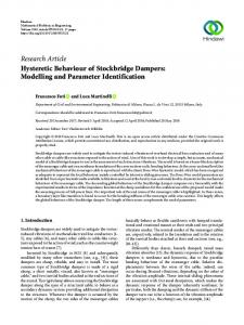
Fig. 1. Given measurements of the joint torques, the set of undetectable changes in inertial parameters is characterized by transfers of inertia, from one body to another, across each joint.

zation of rigid-body kinematics [31], [32], and controllability/observability theory for switched linear systems [33]. As an enabling insight toward developing the RPNA, a main conceptual contribution is to show that all undetectable changes in the inertial parameters can be interpreted as a sequence of inertial transfers across the joints of the mechanism. This powerful observation was made originally in [34] for floating-base systems with a limited set of joint types. It was later independently discovered by Chen et al. [35], [36] and developed further by Ros and colleagues [37], [38], [39]. These recent works have provided many helpful rules of thumb for selecting minimal parameters for particular joint types. Our main contribution is to provide a fully-automatic method that applies these insights to determine the minimal parameters for general joints. To make this notion of an inertia transfer more concrete, consider a revolute joint connecting two bodies, as in Fig. 1, and consider the following modification to the bodies. Suppose a mass m is added to Body i at a point along the axis of Joint i and the same amount of mass m is subtracted from the parent Body i − 1 at the same point along the joint axis. Such a modification will change the inertial parameters of both bodies, however, the kinetic and potential energies of the mechanism (and thus its dynamics) will be unchanged. This operation of adding and subtracting mass represents a transfer of inertia across the joint, and will be shown as the basis for all undetectable changes of parameters in both floating- and fixed-base systems. In fixed-base systems, motion restrictions prevent many inertial parameters from appearing in the dynamics. For example, the first link of a revolute manipulator can only move in its plane of rotation, and thus any parameters capturing out-ofplane effects do not affect the dynamics. A main theoretical contribution of this work is to address the implications of these restrictions on the unidentifiable inertial parameters. We demonstrate a novel application of linear systems theory to accomplish this aim. We first apply recursive linear reachability analysis for the spatial velocities of each link. By understanding the attainable velocities at each link, we can understand the inertial parameters that influence the kinetic energy. With this stepping stone, we then apply linear observability analysis for inertial transfers across each joint. This development plays a key role to determine the transfers that are undetectable via the kinetic energy. A similar approach is applied to determine inertial parameters that do not affect the the generalized gravitational force. Linear systems theory

C. Organization The paper is organized as follows. Section II sets notation and provides rigid-body dynamics preliminaries. Section III introduces the main idea of the recursive parameter-nullspace algorithm for the simplified case of a floating-base system with single-DoF joints. The fact that every link can experience general 6D motion simplifies analysis for this case. Section IV considers the case of fixed-base systems, addressing the role of motion restrictions on the unidentifiable parameters of links near the base. A number of extensions to the basic algorithm are provided in Section V and concluding comments are provided in Section VI. II. P RELIMINARIES A. Mathematical Notation Throughout the text, the set of real and natural numbers are denoted by R and N respectively. R+ represents the set of non-negative reals, while Rn represents the set of n × 1 column vectors with real-valued entries. Similarly Rm×n represents the set of all m × n matrices. Unless otherwise specified, scalars and scalar-valued quantities are denoted with italics (a, b, c, . . .) while vectors and vector-valued functions are denoted with upright bold characters (a, b, c, . . .). Matrix quantities are denoted with upright bold capitals (A, B, . . .). 1n indicates the n × n identity. Definition 1 (Controllability Matrix). Consider the pair (A, B) with A ∈ Rn×n , B ∈ Rn×m . The controllability matrix associated with the pair (A, B) is given by   Ctrb(A, B) = B AB · · · An−1 B The range of the controllability matrix is the smallest Ainvariant subspace of Rn that contains the range of B. Definition 2 (Observability Matrix). Consider the pair (C, A) with A ∈ Rn×n , C ∈ Rp×n . The observability matrix associated with the pair (C, A) is given by   C  CA    Obs(C, A) =   ..   . CAn−1

The nullspace of the observability matrix is the largest Ainvariant subspace within the nullspace of C. B. Rigid-Body Dynamics The treatment of rigid-body dynamics here relies heavily on 6D spatial notation [29], [30]. Spatial notation can be translated to a corresponding Lie-theoretic notation [32], [40].

3

1) Connectivity and Kinematics: Any rigid-body system can be described by a set of N rigid bodies connected by a series of joints. For clarity of exposition, we originally limit description to serial-chain floating-base systems with bodies connected via single degree of freedom joints. Bodies are numbered sequentially from 1 to N going from the floating base to the end of the chain. Joint i is defined to connect Body i − 1 with Body i. The configuration of the base is denoted qB ∈ SE(3), with joint configuration qJ = [q2 , . . . , qN ]T . We collect the system configuration as q = (qB , qJ ). A coordinate frame is attached to each body to describe motion with respect to a local basis. The kinematic relationship between neighboring bodies will be described with the general joint notation in [41]. The spatial velocity of Body i is related to its predecessor though   ωi vi = = i Xi−1 vi−1 + Φi q˙i (1) vi where ω i ∈ R3 the angular velocity in body coordinates, and v i ∈ R3 the linear velocity of the coordinate origin (given in body coordinates). The matrix i Xi−1 is a spatial transformation matrix that converts spatial velocities in frame i−1 to equivalent velocities in frame i. The matrix Φi ∈ R6×1 is a full-column-rank matrix that describes the free mode of motion for joint i. For instance, for a revolute joint following the Denavit-Hartenberg convention Φi = [0, 0, 1, 0, 0, 0]> . As diagrammed in Fig. 2, each joint transformation is composed as a fixed transformation Ji Xi−1 across Body i − 1, followed by a joint transformation i XJi(qi ) i

Xi−1 = i XJi(qi ) Ji Xi−1

(2)

Further, from (1) and [29, Example 2.4] it follows that di Xi−1 = −(Φi q˙i ) × i Xi−1 (3) dt where (v)× : R6 → R6×6 provides the spatial cross product matrix such that     ω S(ω) 0 ×= (4) v S(v) S(ω) with S(x) ∈ R3×3 the skew-symmetric matrix 3D cross product matrix such that S(x)y = x × y for all x, y ∈ R3 . We define the generalized velocity ν as  > ν = v1> q˙ > J 2) Kinetic and Potential Energy: Given a spatial velocity vi for body i its kinetic energy is given by 1 Ti = vi> Ii vi (5) 2 where Ii is the spatial inertial for body i and is given by   ¯Ii mi S(ci ) Ii = (6) mi S(ci )> mi 13 with ci ∈ R3 the CoM of body i in local coordinates, mi ∈ R+ the body mass, and ¯Ii ∈ R3×3 a standard 3D rotational inertia tensor about the coordinate origin. The kinetic energy can be described linearly for a specific

Joint i Body i

i

1

1

Ji Ji

Xi

i

1

X Ji

Body i

i Fig. 2. Joint coordinate systems. Frame Ji is attached to body i − 1 at the joint. Frame i is attached to body i after the joint. Body i is drawn displaced from its actual attachment location for clarity.

parameterization of each Ii . Letting I I I  xx xy xz ¯Ii = Ixy Iyy Iyz Ixz Iyz Izz

(7)

and hi = [hx , hy , hz ]> = mi ci , it follows that the spatial inertia Ii can be expressed linearly in the body inertia parameters π i ∈ R10 π i = [m, hx , hy , hz , Ixx , Ixy , Ixz , Iyy , Iyz , Izz ]>

(8)

To switch between the matrix and parameter vector form of the spatial inertia we employ the notation I(π i ) = [π i ]∧ and π i = [I(π i )]∨ where the wedge ∧ promotes a vector to an inertia matrix, while the vee ∨ demotes an inertia matrix to a parameter vector. Let ek ∈ R10 provide the k-th coordinate vector in R10 . The kinetic energy of Body i can be expressed as Ti =

10 X 1 k=1

2

vi> [ ek ]∧ vi πik

(9)

The time rate of change of the gravitational energy is V˙ i = −

10 X

vi> [ ek ]∧ i X0 0 ag πik

(10)

k=1

which is also linear in π i . Collecting parameters as >  · · · π> π = π> (11) 1 N PN PN we denote V (q, π) = i=1 Vi and T (q, ν, π) = i=1 Ti . 3) Dynamics: The dynamics take the standard form H(q, π) ν˙ + c(q, ν, π) + g(q, π) = τ

(12)

with H ∈ R(N +6)×(N +6) the mass matrix, c ∈ Rnd and g ∈ Rnd the Coriolis and gravity forces, τ ∈ Rnd the generalized force. It can be shown that these quantities satisfy T =

1 > ν Hν 2

and

(13)

∂ V˙ =g (14) ∂ν while c can be computed from partials of H. Due to linearity of each term in π, a regressor matrix Y ∈ R(N +6)×10N [42]

4

Considering when q2 = 0 and 2 XJ2(q2 ) = 16 requires

can be constructed such that ˙ π τ = Y(q, ν, ν)

4) Identifiability of Parameters: To conclude this section we consider structural identifiability of the inertial parameters given a variety of measurements. We introduce the following ˙ ˙ NY = {δπ ∈ R10N | Y(q, ν, ν)δπ = 0, ∀ q, ν, ν} (16) NT = {δπ ∈ R

NH = {δπ ∈ R

Ng = {δπ ∈ R

10N

10N 10N

| T (q, ν, δπ) = 0, ∀ q, ν}

(17)

| g(q, δπ) = 0, ∀ q}

(19)

| H(q, δπ) = 0, ∀ q}

Proposition 1. Given the previous definitions, the structurally unobservable subspaces satisfy NT = NH . Proposition 2. Given the previous definitions, the structurally unobservable subspaces satisfy NY = NH ∩ Ng . III. I DENTIFIABILITY OF I NERTIAL PARAMETERS IN F LOATING -BASE S YSTEMS This section considers unobservable inertial parameters for a floating-base system. We begin by examining a system of two bodies to illustrate the central idea of inertial transfers. We then detail generalization to floating-base serial-chain systems with multiple bodies. These serial-chain results have near-immediate generalizations to the branched tree-structure case, as described in Section V-B. A. Simple Case: Floating-Base System with Two Bodies We begin by considering a floating-base system with two bodies and a single joint. For this system, the mass matrix H takes the simple form " # 2 2 > I1 + 2 X> X 1 I 2 Φ2 1 I2 X 1 H= 2 Φ> Φ> 2 I2 X 1 2 I2 Φ2 We further consider a collection of changes in inertia parameters δπ 1 , δπ 2 , with associated changes to inertia matrices δI1 = [δπ 1 ]∧ and δI2 = [δπ 2 ]∧ . Examining the change to H11 , denoted δH11 , shows δH11 = 0 if and only if (20)

This sum represents the change in the locked inertia of the two bodies. As a result, this condition requires that the combination of δI1 and δI2 must represent an even exchange of inertia between these bodies. Although the inertial changes δI1 and δI2 represent fixed quantities, dependence on configuration in 2 X1(q2 ) requires that the inertia transfer must remain equal and opposite as the joint configuration changes. We build towards making this requirement more mathematically precise. Using the form of from 2 X1 from (2), the equal exchange condition (20) is equivalent to requiring 2 > 2 J2 δI1 + J2 X> 1 XJ2 (q2 ) δI2 XJ2(q2 ) X1 = 0

while considering changes in configuration requires
d 2 > XJ2 δI2 2 XJ2 0= dt
> 2 = −q˙2 2 X> J2 [ (Φi ×) δI2 + δI2 (Φ2 ×) ] XJ2

∀q2 (21)

(22)

(23) (24)

Since 2 XJ2 is full rank, this condition is equivalent to

(18)

which encode structural observability through the generalized force, the kinetic energy, the mass matrix, and the gravitational generalized force respectively.

2 δI1 + 2 X> 1 (q2 ) δI2 X1(q2 ) = 0 ∀q2

J2 δI1 = −J2 X> X1 1 δI2

(15)

(Φ2 ×)> δI2 + δI2 (Φ2 ×) = 0

(25)

This equation may be recognized as requiring a zero time derivative of the spatial inertia δI2 when moving with spatial velocity Φ2 [29, Eq. (2.65)]. Note that the exchange invariance condition (25) is linear δπ 2 . Letting A(Φ2 ) =

∂ [ (Φ2 ×)> [δπ 2 ]∧ + [δπ 2 ]∧ (Φ2 ×) ]∨ (26) ∂δπ 2

the quantity A(Φ2 ) δπ 2 characterizes the rate of change in inertial parameters from the body moving with velocity Φ2 . Thus (25) is equivalent to A(Φ2 ) δπ 2 = 0. Ensuring δH = 0 requires one additional condition in this simplified case. Examining δH12 we see that δH12 = 2 X> 1 δI2 Φ2 = 0 if and only if δI2 Φ2 = 0. (27) This follows since any spatial transform i Xj is full rank. This condition (27) encodes that changes in inertia δI2 must not alter the linear or angular momentum created by joint motions Φ2 . To summarize, for a floating-base system with two bodies, undetectable changes in inertia are exactly those representing a transfer of inertia that does not change with configuration and does not modify momentum J2 δI1 = −J2 X> X1 1 δI2 >

0 = (Φ2 ×) δI2 + δI2 (Φ2 ×) 0 = δI2 Φ2

(Transfer)

(28)

(Invariance)

(29)

(Momentum)

(30)

We name these conditions the transfer condition, the invariance condition, and the momentum condition. Conditions (29) and (30) are equivalent to [7, Eq. (43)]; however, this new form admits greater physical intuition. B. Examples This subsection provides a number of examples with different joint types for intuition into the parameter nullspace of a two-body system. In each case, we only consider parameter changes to Body 2, since the corresponding changes to Body 1 are determined uniquely through the transfer condition (28). 1) Revolute Joint: Consider a revolute joint under the Denavit-Hartenburg convention Φ2 = [0 0 1 0 0 0]> . In this case the momentum condition (30) imposes δIxz = δIyz = δIzz = δhy = δhx = 0

(31)

for the second link. Again, this condition ensures that the parameter variation does not alter the momentum of Body 2 created by joint rotations. Likewise (29) imposes δhy = δhx = δIxy = δIxz = δIyz = δIxx − δIyy = 0 (32)

5

to ensure that an exchange of inertia remains unchanged with joint rotations. As a result, it is observed that δπ 2 has three degrees of freedom through δm, δhz , δIxx = δIyy

(33)

Notation for this third freedom signifies that changes in Ixx must match those to Iyy . In this example, the inertia exchange has a physical interpretation. The transfer freedoms can be thought to represent an exchange of any infinitely thin rod along the joint axis. 2) Prismatic Joint: For a prismatic joint with Φ2 = [0 0 0 0 0 1]> , the unidentifiable inertia exchange takes a different structure. The momentum condition requires δm = δhx = δhy = 0

δπ ∈ NH then δπ ∈ Ng . Thus, for open-chain floating-base systems, changes in parameters do no affect inverse dynamics if and only if they do not affect the mass matrix. Second, it is argued that the parameter nullspace for the mass matrix NH can be determined through consideration of its floating-base rows. A floating-base serial-chain structure has a symmetric mass matrix with upper triangle [30]  C I1   ·  H=   · ·

2

C X> 1 I2 Φ2

C Φ> 2 I2 Φ2

··· ···

·

..

·

·

.

N

C X> 1 IN ΦN



 N C Φ> X> 2 2 IN ΦN    ..  . 

(35)

C Φ> N IN ΦN

where IC i is the composite rigid-body inertia of the subtree rooted at Body i satisfying

while the invariance condition requires IC i =

δm = δhx = δhy = δhz = 0

N X

j

j X> i Ij X i

(36)

j=i

Thus, undetectable inertial transfers across a prismatic joint have six degrees of freedom, admitting changes to any of the rotational mass moments of inertia or mass products of inertia. In this case, these inertial transfers do not have a physical interpretation, but represent any zero-net-mass exchange that leaves the CoM unaltered. 3) Helical Joint: The conditions on undetectable transfers across a helical joint Φ2 = [0 0 σ 0 0 1]> with σ 6= 0 are the intersection of the conditions for a prismatic and a revolute joint. That is, undetectable inertial transfers between two bodies connected by a helical joint have only one degree of freedom following δIxx = δIyy (34) This freedom represents a zero-net-mass exchange along the joint axis that leaves the CoM unchanged. C. Generalization: Floating-Base System with N Links In the two-body example, we saw that the unobservable parameter space for the mass matrix H was determined from conditions on the first block of rows. As it turns out, the full parameter nullspace NY of a floating-base system can be uniquely identified through consideration of the first block of rows in the mass matrix. This, in part, is due to the fact that the first rows of the equations of motion embed the Newton and Euler equations for the entire system [43] and correspondingly, the first rows of the mass matrix encode the net momentum [29], [44]. We build toward the implications of this result for identification in two steps. First, it is argued that the parameter nullspace for the mass matrix NH is contained within the parameter nullspace for the gravitational term Ng . Note that the gravitational term for a floating-base system can be found by considering an gravityfree system, but accelerating opposite gravity and with all joints fixed. That is g(q) = −H(q)ν˙ grav , where  > ν˙ grav = (1 X00 ag )> 0> This trick of accelerating the base to account for gravitational effects is commonly applied in inverse dynamics algorithms to save computation [45]. As a result of this reasoning, if

As a result, (35) shows that any entry in the mass matrix can be computed from the first block row of the mass matrix   2 > C C X 1 I 2 Φ2 · · · N X > (37) H1 = IC 1 1 IN ΦN It follows that changes in the inertial parameters do not affect H1 if and only if they do not affect the inverse dynamics, i.e., NY = NH1 . With this in mind, a nice recent theoretical result [7] may be understood more directly. Intuitively, undetectable transfers in inertia can be chained through a mechanism. That is, since a local inertial transfer across Joint i leaves the composite inertia IC i−1 unchanged, the parameter nullspace for any additional undetectable changes to inertias δI1 , . . . , δIi−1 can be determined independently. The following theorem states this intuition more formally. Theorem 1 (Parameter Nullspace for a Floating-Base System). Consider a floating-base system with sets Ji Ti = {δπ ∈ R10N | δIi−1 = −Ji X> i−1 δIi Xi−1,

0 = δIi Φi ,   0 = (Φi ×)> δIi + δIi (Φi ×) , 0 = δIj if j ∈ / {i, i − 1}}

(38)

for i = 2, . . . , N . The structurally unobservable parameter subspace for the inverse dynamics NY is given by NY = where

L

N M i=2

Ti

(39)

denotes the direct sum of vector subspaces.

Proof. The proof is a special case of arguments in the following sections. IV. I DENTIFIABILITY OF I NERTIAL PARAMETERS IN F IXED -BASE S YSTEMS This section extends the results of the previous section to the case of fixed-base robots. In this case, some of the links may have restricted motion. For instance, a link connected to the fixed base through a revolute joint experiences a limited range of spatial velocities. As a result, its motions excite a

6

Attainable Velocities vi 2 Range(Vi )

This condition is difficult to verify, since it represents an infinite number of conditions across all possible configurations. This challenges motivates the definition of the following set:

i ⇥, VJi )

Vi = span{i Xj(q)Φj | j ≤ i, q ∈ RN }

Vi = [Ctrb(

i]

VJi = Ji Xp(i) Vp(i)

Vp(i)

Fig. 3. Controllability analysis is applied recursively to obtain a basis Vi for the attainable velocities of each body.

limited number of inertial parameters. Toward addressing this feature, we again express the unobservable parameter as the direct sum of unobservable inertia transfers across each joint. By proceeding joint-by-joint, we detail a novel method that transforms the nonlinear parameter observability problem into a sequence of linear observability problems with classical results from linear systems theory [46]. The parameter nullspace NH for the kinetic energy is first characterized. Section IV-B then extends this analysis to address the gravitational term. We conclude the section with a compact description of the Recursive Parameter Nullspace Algorithm (RPNA). A. Observability Analysis for Undetectable Inertial Transfers In the case of robots with motion restrictions, we will again find that unidentifiable changes in the parameters arise from a sequence of transfers across the joints. However, unlike in the case of floating-base systems, these transfers do not need to be invariant with respect to changes in the joint angle. The transfer and invariance conditions at Joint i provided that the composite inertia of the predecessor was unchanged δIC i−1 = 0. When the invariance condition is violated, it is possible that δIC i−1 6= 0 as the configuration changes. Yet, as long as > vi−1 δIC i−1 vi−1 = 0

we will find that this residual effect does not alter the kinetic energy. In this case, even though the transfer is not equal and opposite any longer, its remains undetectable with changes in configuration. We show how classical linear systems theory can be used to address this issue by leveraging the same underpinning mathematics as in the products of exponentials formulation of kinematics [31]. In this fixed-base case, we remove floating-base, and number all bodies from 1 to N . The generalized velocity ν = q˙ J includes only the joint rates, and the mass matrix has its upper triangle given as      H=   

C Φ> 1 I1 Φ1

2 > C Φ> 1 X1 I2 Φ2

·

C Φ> 2 I2 Φ2

···

N C Φ> X> 1 1 IN ΦN

..

.. .

·

·

..

·

·

·

. .



      > N > C ΦN −1 XN −1 IN ΦN   C Φ> N IN ΦN

Suppose a perturbation δπ such that Body i is the largest numbered body with δIi 6= 0. For j ≤ i δHji = 0 requires i > Φ> j Xj (q) δIi Φi = 0 ∀q

(40)

(41)

This span is a linear subspace of R6 . Although (40) represents an infinite number of conditions, if a basis for Vi can be found, these infinite conditions can be checked in a finite manner. The set Vi is named the attainable velocity span and will play a key role in the remainder of the text. The naming is motivated as follows. The velocity of Body i is determined from the joint rates of all its predecessors according to vi =

i X

i

Xj(q) Φj q˙j

j=1

thus Vi is equivalently viewed as the span of all attainable velocities. It is important to note, all attainable velocities for Body i are in Vi , but not all elements of Vi are attainable velocities. However, all elements of Vi can be expressed as the linear combination of some attainable velocities. In this sense, the subspace characterizes the motion restrictions on Body i. The following lemma details how a basis for this span can be propagated across a joint. Lemma 1 (Controllability for Attainable Velocity Spans). Consider a spatial transform as a function of a single angle q, denoted X(q). Suppose X(0) = 1 and further that ∂ X(q) = −Φ × X(q) ∂q

(42)

for some Φ ∈ R6×1 . For any V ∈ R6×k span{v | ∃q ∈ R, v ∈ Range(X(q) V)}

= Range( Ctrb( (Φ×), V ) )

(43) (44)

This gives the span of velocities that can be reached after the joint Φ from velocities in Range(V) before the joint. Proof. See appendix. Corollary 1. Suppose a matrix Vi−1 such that Vi−1 = Range(Vi−1 ). Let VJi = Ji Xi−1Vi−1 . Then Vi = [ Ctrb( (Φi ×), VJi ) Φi ]

(45)

satisfies Vi = Range(Vi ). This corollary provides a powerful building block for determining the motion restrictions at any Body i. Starting from V0 = {0}, the corollary can be applied recursively to characterize all attainable velocity span Vi . If Vi = Range(Vi ), then using (41), (40) is equivalent to Vi> δIi Φi = 0

(46)

It is important to recognize the power of the attainable velocity spans. Eq. (40) is a condition for all q and is impractical to verify computationally as written. In comparison, (46) can be written as a system of linear equations for δπ i . Letting C(Vi , Φi ) =

∂ Vec(Vi> [δπ i ]∧ Φi ) ∂δπ i

(47)

7

Eq. (46) is equivalent to C(Vi , Φi ) δπ i = 0

(48)

Thus far, we have shown how the attainable velocity sets can be used to ensure δHij = 0 for j j δIj Jj

(50)

j=1

This equation can be expanded by noting that Ji = i Xi−1 Ji−1 + Φi Si where Si ∈ R1×N is the selector matrix for joint i. With this observation (50) is expanded as δH

=J> i−1 +



i

X> i−1

i−2 X



i

δIi Xi−1 + δIi−1 Ji−1

i > > > i + J> i−1 Xi−1 δIi Φi Si + Si Φi δIi Xi−1 Ji−1 > + S> i Φi δIi Φi Si

(51)

Due to sparsity patterns, δH = 0 iff

+

i

J> j δIj Jj ,

(52)

j=1

0 =J> i−1 δIi Φi , 0

=Φ> i

and

(53)

δIi Φi

(54)

Conditions (53) and (54) are together equivalent to (46). We proceed to simplify (52). Defining δI0i−1 such that Ji δIi−1 = δI0i−1 − Ji X> i−1 δIi Xi−1

(55)

the requirement (52) is rephrased as 0 = JJ>i +

i

δI0i−1

Ji−1 +

i−2 X




JJi

0 = vJ>i

J> j δIj Jj

(56)

Ji

Xi−1Ji−1 . This requirement (56) holds iff
i > XJi (qi ) δIi i XJi(qi ) − δIi vJi ∀q, q˙ (57)

0 0 = J> i−1 δIi−1 Ji−1 +

i−2 X

Toward simplifying the condition (59) further, we define the following spans for the outer products of attainable velocities ˙ vi (q, q) ˙ > | q, q˙ ∈ RN } Ki = span{vi (q, q) Ji

X> i−1

| Ki−1 ∈ Ki−1 }

(60) (61)

The set Ki is a vector subspace of the 6 × 6 symmetric matrices and has dimension at most 6×7 2 = 21. The use of script K alludes to its role in the nullspace of kinetic energy. Suppose nk Ki has dimension nki and possesses a basis {Ki,l }l=1i . nki−1 Likewise we denote KJi with a basis {KJi ,l }l=1 . Then (59) is equivalent to: (62)

Although this still represents an infinite number of constraints, the reduction from the outer product span KJi provides a step in the right direction. Using a construction similar to the attainable velocity spans, a basis for Ki can be computed recursively. The details of this computation are provided in Appendix A. Note that (62) is satisfied at qi = 0. Thus, (62) holds for all qi iff     d i > i XJi (qi ) δIi XJi(qi ) − δIi (63) 0 = Tr KJi ,l dqi  i
> 0 = Tr KJi ,l i X> Ji (qi ) (Φi ×) δIi + δIi (Φi ×) XJi(qi )

j=1

where JJi =

In a sense ∆Ii measures the change in inertia transfer across the joint, and it is zero when the transfer is invariant. When any velocity vJi can be attained, (59) is equivalent to the transfer invariance condition from the floating-base case.

That is,

i X> Ji (qi ) δIi XJi(qi ) − δIi

J> i−1

(59)

where Tr(·) gives the trace of a matrix and ∆Ii is defined as
i ∆Ii (qi ) = i X> Ji (qi ) δIi XJi(qi ) − δIi

Tr (KJi ,l ∆Ii (qi )) = 0 ∀qi ∈ R, l = 1, . . . , nki−1

 i X> i−1 δIi Xi−1 + δIi−1 Ji−1

i−2 X

0 = vJ>i ∆Ii (qi ) vJi = Tr(vJi vJ>i ∆Ii (qi )) ∀q, q˙

KJi = span{ Xi−1 Ki−1

j=1



The conditions from (57) are impossible to enforce as written since they represent an infinite number of constraints. To simplify these conditions, we make use of a span, similar to as before. Note that the attainable velocity span cannot be immediately applied, since the condition (57) is not linear in vJi . We write (57) in a rearranged form

Ji

J> j δIj Jj

0 =J> i−1

sideration of inertia exchanges across Joint i from subsequent exchanges across lower numbered joints.

J> j δIj Jj

(58)

j=1

where vJi = Ji Xi−1vi−1 . The second condition (58) is equivalent to requiring δH = 0 for changes δI1 , . . . , δIi−2 , δI0i−1 . Thus the substitution (55) enables a decoupling between con-

∀qi ∈ R, l = 1, . . . , nki−1

(64)

Physically, this condition enforces that changes in the inertia transfer with joint angle do not alter the kinetic energy. Toward simplifying this condition, we introduce the following lemma, which is dual in spirit to Lemma 1. Lemma 2 (Observability Analysis of Inertial Parameters). Consider a spatial transform as a function of a single angle q, denoted X(q). Suppose X(0) = 1 and consider Φ ∈ R6×1 such that ∂ X(q) = −Φ × X(q) (65) ∂q

8

Kinetic Energy Observability Matrix

H OH i = Obs( C i , A(

+ Ii

i) )

Kinetic Energy Nullspace Condition

OH i A(

i)

joint configuration. Here instead, limitations on the attainable velocities both relax and complicate these constraints. Inertia transfers no longer have to be invariant with changes in joint configuration. However, (70) requires that any changes to the inertial transfer with configuration must not alter the kinetic energy. Combining the results of (46), (55), and (70) proves the following theorem.

i

⇡i = 0

i X> Ji Ii XJi

Theorem 2 (Parameter Nullspace for Kinetic Energy in a Fixed-Base System). Consider a fixed-base system with the following fundamental sets Fig. 4. Observability analysis is applied using motion subspaces VJi to characterize transfers δπ i across Joint i that leave kinetic energy unchanged.

Ti = {δπ ∈ R10N | δπ 0 ∈ R10 ,

Ji δIi−1 = −Ji X> i−1 δIi Xi−1,

0 = Vi> δIi Φi ,   (k) 0 = Tr KJi ,l δIi ,

For any K ∈ R6×6 , define I(Φ, K) =

∀k = 1, . . . , 10, l = 1, . . . , nki−1

{π ∈ R10 | Tr(K X>(q) [π]∧ X(q)) = 0, ∀q ∈ R} (66)

as the set of all inertial parameters that maintain a zero output with respect to K following transformation across a joint with free modes Φ. Then, letting CTr (K) :=

∂ Tr(K [π]∧ ) ∂π

0 = δIj if j ∈ / {i, i − 1}}

for i = 1, . . . , N . The parameter variation δπ 0 represents a free change in the inertial parameters of the base. The structurally unobservable parameter subspace for the kinetic energy NH satisfies NH =

I(Φ, K) = Null ( Obs ( CTr (K), A(Φ) ) ) Proof. See Appendix. This Lemma is critical, in that it enables the infinite number of conditions (64) to be verified via a finite set of linear equalities for δπ i . The outputs from all outer products KJi ,l can be collected as   CTr (KJi ,1 )   .. CH (67)  i = .

(71)

N M i=1

Ti

(72)

Proof. We argue by induction on j, where j denotes the highest numbered body such that δIj 6= 0. In the base Case (j = 1) δH11 is the only variation to δH. The variation δH11 = 0 iff Φ> 1 δI1 Φ1 = 0. In this case, V1 = Φ1 , VJ1 is empty, and nk0 = 0. Thus, T1 has the proper form, and the base case is proven. The main derivation of this section proves the inductive step.

CTr ( KJi ,nki−1 ) With this output matrix, a kinetic energy observability matrix associated with Joint i is defined by OH i

=

Obs( CH i ,

A(Φi ) )

(68)

It then follows that Eq. (64) is satisfied if and only if OH i A(Φi ) δπ i = 0

(69)

This main result is diagrammed in Figure 4. To promote broader understanding of condition (69), we note that it is equivalent to requiring (k) Tr(KJi ,l δIi ) (0)

where δIi

∀k = 1, ..., 10

(70)

= δIi and

(k)

δIi

=0

(k−1)

= [(Φi ×)T δIi (k)

(k−1)

+ δIi

(Φi ×)]

Roughly, each δIi provides the k-th derivative of the inertial transfer with respect to joint configuration. We note than in the floating-base case, the entries KJi ,l span the space of all symmetric 6 × 6 matrices, and thus (70) holds iff (1) δIi = 0. That is, the inertial transfer must not change with

B. Gravity Consideration Similar to the previous subsection, unobservable parameters in Ng can be determined through recursive application of controllability and observability considerations outward through the tree. Using the form of the generalized gravitational force from (14) and (10) δg = −

N X

j 0 J> j δIj X0 ag = 0

j=1

Each entry of the sum quantifies the change in the instantaneous power of the gravitational force on Body j. Again assuming that Body i is the largest body with δIi 6= 0, and following similar approaches to the previous subsection, define δI0i−1 such that Ji δIi−1 = δI0i−1 − Ji X> i−1 δIi Xpi

Then, it can be shown that δg = 0 iff i > 0 = 0 a> g X0 δIi Φi

0=

vJ>i

(

i

i X> Ji (qi ) δIi XJi(qi )

(73) Ji

0

− δIi ) X0 ag

(74)

9

˙ and subsequent changes δI1 , . . . , δIi−2 , δI0i−1 for all q, q, independently satisfy δg = 0. Condition (73) motivates definition of the attainable gravity vector span  Ai = span i X0(q) 0 ag | q ∈ RN Akin to the propagation of attainable velocity spans, we seed A0 = 0 ag , define AJi = Ji Xi−1 Ai−1 and recursively apply

which ensures each Range(Ai ) = Ai . With this propagation, (73) is equivalent to requiring (75)

Examining (74) in further detail, it holds iff
0 = Tr Ji ag vJ>i ∆Ii (qi )

(76)

In this sprit, we define the following set, analgous to Ki , for the gravitational power | q, q˙ ∈ RN }

(78)

Denoting the dimension of Pi as npi , the appendix details a np recusive method to compute a basis {Pi,l }l=1i . Similar to the observability analysis for the kinetic energy, we denote an output matrix for the gravitational power as   CTr (PJi ,1 )   .. (79) Cgi =   . CTr ( PJi ,npi−1 ) and define the observability matrix for the gravitational power Ogi = Obs( Cgi , A(Φi ) )

(80)

Eq. (74) is equivalent to Ogi A(Φi ) δπ i = 0

(81)

which denotes that any changes in the inertial transfer, A(Φi ) δπ i , must be unobservable to the gravitational power. We collect the gravitational and kinetic conditions " g# Ci Ci = (82) CH i Oi = Obs( Ci , A(Φi ) )

Ti = {δπ ∈ R10N | δπ 0 ∈ R10 ,

Ji δIi−1 = −Ji X> i−1 δIi Xi−1,

0 = A> i δIi Φi , (k)

0 = Tr(Ki,l1 δIi ), ∀l1 = 1, . . . , nki−1 (k)

0 = Tr(Pi,l2 δIi ), ∀l2 = 1, . . . , npi−1 , ∀k = 1, . . . , 10

for any attainable vJi and Ji ag = Ji X00 ag . Yet, since ∆Ii is symmetric this holds if and only if

0 = Tr Ji ag vJ>i + vJi Ji a> ∆Ii (qi ) (77) g

˙ > +vi (q, q) ˙ i ag (q)> Pi = span{ i ag (q) vi (q, q)

Theorem 3. Consider a fixed-base system with the following fundamental sets

0 = Vi> δIi Φi ,

Ai = Ctrb( (Φi ×), AJi )

ATi δIi Φi = 0

Inductive application of the main derivation of this section allows us to state the following main theorem.

(83)

Remark 1. While we proceed to analyze NY , one might reasonably be interested to consider Ng on its own. This gravitational nullspace corresponds to the parameter nullspace for static experiments. Comparing Ng and NY has the opportunity to provide insight into the parameters that require dynamic experiments to for accurate identification. A quasistatic robot might reasonably be modeled ignoring parameter combinations in Ng .

0 = δIj = 0 if j ∈ / {i, i − 1} }

(84)

for i = 1, . . . , N . The structurally unobservable parameter subspace for the inverse dynamics NY satisfies NY =

N M i=1

Ti

(85)

Proof. Proof follows the same argument as Theorem 2. Alternately, each Ti can be represented by conditions on δπ. Let
∂ Ji > B Ji Xi−1 = [ Xi−1 [ δπ i ]∧Ji Xi−1]∨ (86) ∂δπ i denote the matrix that transforms inertial param backwards to the predecessor. Using this matrix,
Ti = {δπ | δπ 0 ∈ R10 , δπ i−1 = −B Ji Xi−1 δπ i , 0 = Ni δπ i

0 = δπ j = 0 if j ∈ / {i, i − 1} }

(87)

where the nullspace descriptor Ni can be formed by collecting the requirements from (48) and (69) for the kinetic energy nullspace with (75) and (81) for the gravitational nullspace. " # C([Vi Ai ], Φi ) Ni = (88) Oi A(Φi ) Algorithm 1 provides a compact method to recursively compute the parameter nullspace descriptors Ni . We name this method the Recursive Parameter Nullspace Algorithm (RPNA) due to its recursive structure that proceeds outward through the kinematic tree. As a practical matter, linearly dependent columns of Vi or Ai can be removed at any step in the algorithm. Likewise, linearly dependent rows of each Ci or Oi can be removed at any step. These modifications minimize the size of each Ni without impact on its nullspace. A M ATLAB implementation of this algorithm is provided in the supplementary material. Remark 2. From the form of Algorithm 1, it may be observed that there are only a few minor differences in the propagation of Vi compared to Ai and Ki compared to Pi . As a result, a combined basis for [Vi , Ai ] can be obtained by simply seeding V0 = 0 ag , and then removing Ai entirely. With this modification Ki + Pi will be captured in the new Ki , and

10

Pi can be likewise removed from the algorithm. In a sense, this modification corresponds the addition of a prismatic joint aligned with gravity at the base whose force is not measured. V. E XTENSIONS This section considers a number of extensions to the RPNA algorithm that follow readily from the previous developments. We first consider a generalization to multi-DoF joints, unifying the treatment of floating-base and grounded cases, as well as opening possibilities for general joint structures. The second subsection comments on generalization to tree-structure systems, while the final-subsection offers preliminary remarks on generalization to closed-loop systems. In particular, we examine the identifiability of motor components, which imposes perhaps both the simplest and most common closed loop found in conventional robots.

Algorithm 1: Recursive Parameter Nullspace Algorithm (RPNA) 0 1 A0 = a g 2

V0 = 06

3

K0 = {06×6 }

4 5 6 7 8 9 10 11 12 13 14

A. Generalization to Multi-DoF Joints and Tree-Structure Systems In generalizing the RPNA to multiple DoF Joints, we suppose that each joint has configuration manifold Qi of dimension ndi . The generalized velocity of each joint is given as ν i ∈ Rndi . We express the free modes of the joint h i Φi = φi,1 · · · φi,nd

15

16

17 18

P0 = {06×6 }

for i = 1, . . . , N do VJi ← Ji Xi−1 Vi−1

AJi ← Ji Xi−1 Ai−1

Vi ← [Ctrb((Φi ×), VJi ) Φi ] Ai ← Ctrb((Φi ×), AJi )

Ki = PropagateBasis(Ki−1 , Ji Xi−1, Φi ) + ColumnOuterProducts(Φi , Vi ) Pi = PropagateBasis(Pi−1 , Ji Xi−1, Φi ) + ColumnOuterProducts(Φi , Ai ) Oi = Obs( Ci , A(Φi ) ) # " C([Vi , Ai ], Φi ) Ni = Oi A(Φi ) end return Ni ,

i = 1, . . . , N

i

6

where each φi,j ∈ R is fixed. With this convention the velocity propagation (1) takes the form vi = i Xi−1vi−1 + Φi ν i

(89)

We first consider the case of a floating-base system with multi-DoF joints. The intertial transfer nullspace at each joint in a floating-base system is determined by the intersection of a momentum condition, a transfer condition, and a transfer invariance condition. Transfer invariance (29) is generalized for all possible joint rates by enforcing 0 = (φi,j ×)> δIi + δIi (φi,j ×) ∀j ∈ {1, . . . , ndi } while the momentum condition (30) generalizes directly. The transfer condition is unaffected by the structure or number of the joint free modes. When moving to the fixed-base case, the propagation of the attainable velocity spans via Corrolary 1 can be generalized using a generalization of controllability for switched linear systems. It is noted the kinematics across a single-DoF joint follow a linear system (42). In contrast, across a multi-DoF joint with Φi = [φi,1 , . . . , φi,nd ] i n o di XJi(qi ) ∈ span (φi,1 ×) i XJi, . . . , (φi,nd ×) i XJi i dt As a result, the set span{v | ∃qi ∈ Qi , v ∈ Range(i XJi(qi ) V)} can be seen as the smallest set containing Range(V) that is invariant under each (φi,k ×). This set is equivalent to the controllable subspace of a switched linear system [33] with

nd

i pairs { ( (φi,k ×), V ) }k=1 . If the controllability matrix in the propagation of the velocity span for the single-DoF case

Vi = [ Ctrb( (Φi ×), VJi ) Φi ] is replaced with any matrix whose range equals the switched controllable subspace of these pairs, then Corollary 1 holds for multi-DoF joints. The propagation of the outer product spans Ki generalize through an identical switched controllability construction. Likewise, the observability conditions for the kinetic energy (69) and gravitational power (80) generalize to the multi-DoF joint case through a switched-linear systems observability condition. One can consider the switched observable subspace ndi with pairs { ( Ci , A( φi,k ) ) }k=1 . This switched unobservable subspace is the largest subspace of Null(Ci ) that is invariant under each A( φi,k ). If the observability matrix Oi is replaced by any matrix whose nullspace coincides with this switched unobservable subspace, then the condition (69) is generalized as   Oi A(φi,1 )   ..   δπ i = 0 . Oi A(φi,nd ) i

B. Generalization to Tree Structure Systems Although the main body of the manuscript has dealt with unbranched serial chains, it decomposed the parameter nullspace into a sequence of transfers across joints. This decomposition readily generalizes to the branched case. In the

11

branched system, we number bodies 1 to N in a way such the predecessor of body i, denoted p(i), is numbered less than i. In this case the transfer condition in the fundamental set Ti of (84) is re-written as

Rotational symmetry of the rotor implies Ixz = Iyz = hx = hy = 0 and Ixx = Iyy . Intuitively, such symmetry implies

Ji δIp(i) = −Ji X> p(i) δIi Xp(i)

Thus, the transfer invariance (92), momentum (93), and torque (94) conditions simplify to

All outward propagations for vi in (1), Vi in (45) etc. generalize by likewise replacing i − 1 with p(i). C. Generalization to Closed Kinematic-Loops: A Preliminary Example This subsection considers generalization to address identifiability of motor rotors, which is perhaps the simplest case of a closed kinematic loop. Motors present a closed kinematic loop because a motor at Joint i is attached both to Body p(i) and Body i. Toward understanding this case, we consider a three body system with floating-base (Body 1), a motor (Body m), one additional body (Body 2). We first break the constraint connecting the motor to Body 2 and consider the open chain system with joint angles qJ = [qm , q2 ]> . This system has mass matrix  C m >  I1 X1 Im Φm 2 X> 1 I 2 Φ2  0 Φ> H= · (90) m Im Φm > · · Φ2 I2 Φ2

0 = (Φm ×)> δIm + δIm (Φm ×)

0 = (Φ2 ×)> δI2 + δI2 (Φ2 ×) 0 = δIzzm

T

The mass matrix in these new coordinates is given by # " C m > I1 X1 Im Φm nR + 2 X> 1 I2 Φ2 0 > H = T HT = > 2 · Φ> m Im Φm nR + Φ2 I2 Φ2

δIzzm

0=

δIm Φm nR +

X> 1

δI2 Φ2

(97)

nR2

+

Φ> 2

(98)

δI2 Φ2 = 0

(99)

This document has introduced the recursive parameter nullspace algorithm (RPNA) to compute the inertial parameter nullspace in rigid-body system identification. We have show than unidentifiable parameter combinations have an interpretation as representing a sequence of inertial transfers across the joints. In arriving at this result, we have transformed the nonlinear parameter observability problem of determining NY into a sequence of classical linear systems observability problems. Extensions have been discussed to handle general multi-DoF joint models, branched kinematic trees, and simple closed loops arising from geared motors. Future developments will provide detailed examples of this method applied to a grounded and floating-base systems. A PPENDIX A S ELECTED P ROOFS

(91)

A. Proof of Lemma 1 (92) (93)

These conditions guarantee that the variation to the first block row is zero. However, unlike the open-chain floating-base case, a zero variation to the first block row does not imply a zero variation to the remainder to H0 . The entry H022 requires > 2 0 = Φ> m δIm Φm nR + Φ2 δI2 Φ2

δI2 Φ2

Thus, these equations can be satisfied (and δIzz is unidentifiable) when the gear ratio is unity, Joint 2 is rotational, and its axis is parallel to the motor axis. Note that this condition allows the motor to be offset from the joint. In all other cases, the rotor adds one identifiable parameter Izzm . Future work will extend this analysis to fixed-base systems.

The inertia transfer, transfer invariance, and momentum conditions are generalized as

J2

(96)

VI. C ONCLUSIONS

We consider a change of coordinates that accounts for the constraint between qm and q2 . In the case of a gear ratio nR such that qm = nR q2 , we use ν 0 = [v1> , q2 ]>   1 0 ν =  0 nR  ν 0 0 1 | {z }

X> 1

+

Φ> 2

Jm > Φ> XJ2 Φm δIzzm nR + Φ> 2 2 δI2 Φ2 = 0

m > m 2 > 2 IC 1 = I1 + X1 Im X1 + X1 I2 X1

Jm

nR2

Since δIzzm is the only term appearing, the motor can add one additional identifiable parameter at most. However, there are conditions when the motor rotor cannot be identified. The only way (96) and (97) can be satisfied simultaneously is if

where

Jm J2 δI1 = − Jm X> X1 − J2 X> 1 δIm 1 δI2 X1   Jm > 0 =J m X > X1 1 (Φm ×) δIm + δIm (Φm ×)   J2 J2 > > + X2 (Φ2 ×) δI2 + δI2 (Φ2 ×) X1

(95)

J2 > X1 δI2 Φ2 0 = Jm X> 1 Φm δIzzm nR +

(94)

which we refer to as the torque condition. In the common case that motor rotors are rotationally symmetric, these conditions simplify a great deal. Consider a motor rotating about its z axis such that Φm = [0, 0, 1, 0, 0, 0]> .

Proof. We define S(Φ, V) = span{X(q)v | v ∈ Range(V)} and recall, from the Lemma statement, that d X(q) = −(Φ×)X(q) dq From the definition of the matrix exponential for a linear system [46]: X(q)V = e −q(Φ×) V The Cayley-Hamilton theorem then ensures that S(Φ, V) ⊆ Range [V, (Φ×)V, . . . , (Φ×)5 V]




12

and thus

Letting h i ∗ ∗ Bi = [KJi ,1 ]∨ · · · , [KJi ,nki−1 ]∨

S(Φ, V) ⊆ Range( Ctrb((Φ×), V) ) Note that the range of the controllability matrix provides the smallest (Φ×)-invariant subspace containing Range(V). Yet, S(Φ, V) is invariant under (Φ×) and contains Range(V). This proves the reverse containment.

It follows that

B. Propagation of the Basis for Ki This section details a method to propagate a basis for the attainable outer product span

Thus, any basis for the range of the controllability matrix can be used to generate a basis for the span.

Akin to the propagation of the atatinable velocity span, this can be broken down into components that account for the local joint kinematics and the local joint velocities =

=

span{vi vi> } span{(i Xi−1vi−1 + Φi q˙i )(i Xi−1vi−1 + Φi q˙i )> } > i > > span{i Xi−1vi−1 vi−1 Xi−1 } + span{vi Φ> i + Φi vi }

(100)

A finite basis for elements of the second part of (100) can be computed using each column of Vi from the attainable velocity span. The first part of (100) can be computed using controllability analysis across a joint, following identical arguments as elsewhere in this paper. Since Ki is a vector space of symmetric 6 × 6 matrices, any entry K ∈ Ki can be represented by a vector of 21 elements, denoted as k ∈ R21 .1 Similar to with spatial inertias, use use ∧∗

K = [k]

and k = [K]

KJi ,l = Ji Xi−1 Ki−1,l Ji X> i−1

=span{i XJi(qi ) KJi ,l i XJi(qi ) | qi ∈ R, l = 1, . . . , nki−1 } Toward simplifying this span, we denote the following operation that characterizes the change in parameters k for K when transformed across a joint with free modes Φ. ∂ ∨∗ [(Φ×)[k]∧∗ + [k]∧∗ (Φ×)] ∂k

It follows that h

XJi(qi ) KJi ,l XJi(qi ) = e

(102)

Proof. Let π 0 ∈ R10 and denote

π(q) = [ X>(q) [π 0 ]∧ X(q) ]∨

as the inertial parameters after transfer across a joint. Due to the linearity of [·]∨ , it follows that
d π(q) = −[ X>(q) (Φ×)> [π 0 ]∧ + [π 0 ]∧ (Φ×) X(q) ]∨ dq (103) Since X(q) = e−(Φ×)q , it follows that the spatial cross product (Φ×) commutes with X(q) (Φ×)X(q) = X(q)(Φ×) Combining (103) and (104)  ∨ d π(q) = − (Φ×)> [π(q)]∧ + [π(q)]∧ (Φ×) dq = −A(Φ) π(q)

(104)

(105) (106)

and as a result, Similar to the proof of Lemma 1, the Caley-Hamilton Theorem ensures π(q) ∈ span(π 0 , A(Φ) π 0 , . . . , A(Φ)9 π 0 )

(107)

If π 0 ∈ Null ( Obs ( CTr (K) , A(Φ) ) ), this implies (108)

Combining (107) and (108) then provides Tr(K [ π(q) ]∧ ) = 0 for all q. As a result

> i > span{i Xi−1vi−1 vi−1 Xi−1 }

i

| k ∈ Range(Ctrb(AK (Φi ), Bi ))}

Tr( K [A(Φ)k δπ 0 ]∧ ) = 0 ∀k ∈ 0, . . . , 9

Then, we can compute span

i

=span{[k]

(101)

π(q) = e−A(Φ)q π 0

∨∗

to denote transformations between the matrix and vector representations. nk We suppose a basis for Ki−1 as {Ki−1,l }l=1i−1 and define the transformation of this basis to Joint i through

AK (Φ) =

∧∗

C. Proof of Lemma 2

˙ i (q, q) ˙ > | q, q˙ ∈ RN Ki = span{vi (q, q)v

Ki =

> i > span{i Xi−1vi−1 vi−1 Xi−1 }

−AK (Φi )

[KJi ,l ]

∨∗

i∧∗

1 Note that elements of K ∈ K are used to induce an inner product with a i spatial inertia Tr(K δI), and that spatial inertias represent a 10 dimensional vector subspace of the 6 × 6 symmetric matrices. As a result, K can be viewed an element in the dual of the vector subspace of inertia matrices. Since this dual space has dimension 10 as well, K can be expressed with respect to a 10 element dual basis. This compact representation is used in the attached MATLAB code.

Null ( Obs ( CTr (K) , A(Φ) ) ) ⊆ I(Φ, L1 , L2 ) Note that Null ( Obs ( CTr (K) , A(Φ) ) ) is the largest A(Φ)-invariant subspace contained in Null(CTr (K)). Since I(Φ, K) is A(Φ)-invariant and contained in Null( CTr (K) ), this proves the reverse containment. D. Propagation of the Basis for Pi

For simplicity, we leave each step of the span without taking the symmetric part, as it can be taken at the end without affecting the result. Pi = span{vi i ag }

= span{(i Xi−1vi−1 + Φi q˙i )(i Xi−1i−1 ag )> }

i i > = span{i Xi−1vi−1 i−1 a> g Xi−1} + span{Φi ag }

13

Again the first part can be computed with controllability analysis and the predecessor set Pi−1 , while the second part can be computed from any basis Ai for the attainable gravity vector span Ai . R EFERENCES [1] C. G. Atkeson, C. H. An, and J. M. Hollerbach, “Estimation of inertial parameters of manipulator loads and links,” The International Journal of Robotics Research, vol. 5, no. 3, pp. 101–119, 1986. [2] F. B. W. Khalil, “Symbolic calculation of the base inertial parameters of closed-loop robots,” J. Robotics Res, vol. 14, pp. 112–128, 1995. [3] J. Swevers, C. Ganseman, D. B. Tukel, J. de Schutter, and H. V. Brussel, “Optimal robot excitation and identification,” IEEE Transactions on Robotics and Automation, vol. 13, no. 5, pp. 730–740, Oct 1997. [4] K. Ayusawa, G. Venture, and Y. Nakamura, “Identification of the inertial parameters of a humanoid robot using unactuated dynamics of the base link,” in IEEE RAS Humanoids, Dec 2008, pp. 1–7. [5] ——, “Identification of flying humanoids and humans,” in 2010 IEEE International Conference on Robotics and Automation, May 2010, pp. 3715–3720. [6] K. Ayusawa and Y. Nakamura, “Identification of standard inertial parameters for large-dof robots considering physical consistency,” in 2010 IEEE/RSJ International Conference on Intelligent Robots and Systems, Oct 2010, pp. 6194–6201. [7] K. Ayusawa, G. Venture, and Y. Nakamura, “Identifiability and identification of inertial parameters using the underactuated base-link dynamics for legged multibody systems,” Int. J. of Robotics Research, vol. 33, no. 3, pp. 446–468, 2014. [8] J. Jovic, A. Escande, K. Ayusawa, E. Yoshida, A. Kheddar, and G. Venture, “Humanoid and human inertia parameter identification using hierarchical optimization,” IEEE Transactions on Robotics, vol. 32, no. 3, pp. 726–735, June 2016. [9] J.-J. Slotine and W. Li, “Adaptive robot control: A new perspective,” in Decision and Control, 1987. 26th IEEE Conference on, vol. 26, Dec 1987, pp. 192–198. [10] J.-J. E. Slotine and W. Li, “Composite adaptive control of robot manipulators,” Automatica, vol. 25, no. 4, pp. 509 – 519, 1989. [11] K. Bouyarmane, J. Vaillant, F. Keith, and A. Kheddar, “Exploring humanoid robots locomotion capabilities in virtual disaster response scenarios,” in Humanoid Robots (Humanoids), 2012 12th IEEE-RAS International Conference on, Nov 2012, pp. 337–342. [12] L. Righetti, J. Buchli, M. Mistry, M. Kalakrishnan, and S. Schaal, “Optimal distribution of contact forces with inverse dynamics control,” The Int. Journal of Robotics Research, no. Online First, 2013. [13] S. Kuindersma, R. Deits, M. Fallon, A. Valenzuela, H. Dai, F. Permenter, T. Koolen, P. Marion, and R. Tedrake, “Optimization-based locomotion planning, estimation, and control design for the atlas humanoid robot,” Autonomous Robots, pp. 1–27, 2015. [14] J. Park and O. Khatib, “Contact consistent control framework for humanoid robots,” in Proc. of the IEEE Int. Conference on Robotics and Automation, May 2006, pp. 1963–1969. [15] Y. Abe, M. da Silva, and J. Popovi´c, “Multiobjective control with frictional contacts,” in 2007 ACM SIGGRAPH/Eurographics Symp. on Computer Animation, Aire-la-Ville, Switzerland, 2007, pp. 249–258. [16] J. Park, J. Haan, and F. Park, “Convex optimization algorithms for active balancing of humanoid robots,” IEEE Transactions on Robotics, vol. 23, no. 4, pp. 817–822, Aug. 2007. [17] L. Sentis, J. Park, and O. Khatib, “Compliant control of multicontact and center-of-mass behaviors in humanoid robots,” IEEE Trans. on Robotics, vol. 26, no. 3, pp. 483–501, June 2010. [18] P. M. Wensing and D. E. Orin, “Generation of dynamic humanoid behaviors through task-space control with conic optimization,” in IEEE Int. Conf. on Rob. and Automation, May 2013, pp. 3103–3109. [19] B. R and A. K. J, “On structural identifiability,” Mathematical Biosciences, vol. 7, pp. 329–339, 1970. [20] W. Khalil, J. Kleinfinger, and M. Gautier, “Reducing the computational burden of the dynamic models of robots,” in Proceedings. 1986 IEEE International Conference on Robotics and Automation, vol. 3, Apr 1986, pp. 525–531. [21] M. Gautier and W. Khalil, “A direct determination of minimum inertial parameters of robots,” in Proceedings. 1988 IEEE International Conference on Robotics and Automation, Apr 1988, pp. 1682–1687 vol.3. [22] ——, “Identification of the minimum inertial parameters of robots,” in Proceedings, 1989 International Conference on Robotics and Automation, May 1989, pp. 1529–1534 vol.3.

[23] M. Gautier, “Numerical calculation of the base inertial parameters of robots,” in Proceedings., IEEE International Conference on Robotics and Automation, May 1990, pp. 1020–1025 vol.2. [24] M. Gautier and W. Khalil, “Direct calculation of minimum set of inertial parameters of serial robots,” IEEE Transactions on Robotics and Automation, vol. 6, no. 3, pp. 368–373, Jun 1990. [25] H. Mayeda, K. Yoshida, and K. Osuka, “Base parameters of manipulator dynamic models,” IEEE Transactions on Robotics and Automation, vol. 6, no. 3, pp. 312–321, Jun 1990. [26] H. Kawasaki, Y. Beniya, and K. Kanzaki, “Minimum dynamics parameters of tree structure robot models,” in Industrial Electronics, Control and Instrumentation, 1991. Proceedings. IECON ’91., 1991 International Conference on, Oct 1991, pp. 1100–1105 vol.2. [27] S.-Y. Sheu and M. W. Walker, “Identifying the independent inertial parameter space of robot manipulators,” The International Journal of Robotics Research, vol. 10, no. 6, pp. 668–683, 1991. [28] M. Gautier, “Numerical calculation of the base inertial parameters,” J Robotics Syst., vol. 8, pp. 485–506 (, 1991. [29] R. Featherstone, Rigid Body Dynamics Algorithms. Springer, 2008. [30] R. Featherstone and D. Orin, “Chapter 2: Dynamics,” in Springer Handbook of Robotics, B. Siciliano and O. Khatib, Eds. New York: Springer, 2008. [31] R. W. Brockett, Robotic manipulators and the product of exponentials formula. Berlin, Heidelberg: Springer Berlin Heidelberg, 1984, pp. 120–129. [32] F. Park, J. Bobrow, and S. Ploen, “A lie group formulation of robot dynamics,” The International Journal of Robotics Research, vol. 14, no. 6, pp. 609–618, 1995. [33] Z. Sun, S. Ge, and T. Lee, “Controllability and reachability criteria for switched linear systems,” Automatica, vol. 38, no. 5, pp. 775 – 786, 2002. [34] G. D. Niemeyer, “Computational algorithms for adaptive robot control,” Master’s thesis, MIT, 1990. [35] K. Chen, D. G. Beale, and D. Wang, “A new method to determine the base inertial parameters of planar mechanisms,” Mechanism and Machine Theory, vol. 37, no. 9, pp. 971 – 984, 2002. [36] K. Chen and D. G. Beale, “A new symbolic method to determine base inertia parameters for general spatial mechanisms,” no. 36223, pp. 731– 735, 2002. [37] J. Ros, A. Plaza, X. Iriarte, and J. Aginaga, “Inertia transfer concept based general method for the determination of the base inertial parameters,” Multibody System Dynamics, vol. 34, no. 4, pp. 327–347, Aug 2015. [38] J. Ros, X. Iriarte, and V. Mata, “3d inertia transfer concept and symbolic determination of the base inertial parameters,” Mechanism and Machine Theory, vol. 49, no. Supplement C, pp. 284 – 297, 2012. [39] X. Iriarte, J. Ros, F. Valero, V. Mata, and J. Aginaga, “Symbolic calculation of the base inertial parameters of a low mobility mechanism,” in Proc. ECCOMAS Multibody Dynamics, 2013, pp. 1113–1124. [40] S. Traversaro and A. Saccon, “Multibody dynamics notation,” Technische Universiteit Eindhoven, Tech. Rep., 2016. [Online]. Available: http://repository.tue.nl/849895 [41] R. E. Roberson and R. Schwertassek, Dynamics of Multibody Systems. Berlin/Heidelberg/New York: Springer-Verlag, 1988. [42] J.-J. E. Slotine and W. Li, “On the adaptive control of robot manipulators,” Int. J. of Robotics Research, vol. 6, no. 3, pp. 49–59, 1987. [43] P.-B. Wieber, “Holonomy and nonholonomy in the dynamics of articulated motion,” in Fast Motions in Biomechanics and Robotics, ser. Lecture Notes in Control and Information Sciences, M. Diehl and K. Mombaur, Eds. Berlin/Heidelberg/New York: Springer Berlin, 2006, vol. 340, pp. 411–425. [44] P. M. Wensing and D. E. Orin, “Improved computation of the humanoid centroidal dynamics and application in dynamic whole-body control,” International Journal of Humanoid Robotics (Special Issue on WholeBody Control), vol. 13, pp. 1 550 039:1–23, 2015. [45] R. Featherstone and D. Orin, “Robot dynamics: equations and algorithms,” in Robotics and Automation, 2000. Proceedings. ICRA ’00. IEEE International Conference on, vol. 1, 2000, pp. 826 –834 vol.1. [46] W. J. Rugh, Linear Systems Theory, 2nd ed. Prentice-Hall, Inc., 1996.