pendulum clocks, we find that observing sufficient information to track the build up of synchrony is an ill-posed problem unless measurements are taken from a ...
Joint 48th IEEE Conference on Decision and Control and 28th Chinese Control Conference Shanghai, P.R. China, December 16-18, 2009
ThA11.5
Observability Issues in Networked Clocks with Applications to Epilepsy Elma O’Sullivan-Greene, GSMIEEE, Iven Mareels, FIEEE, Anthony Burkitt, SMIEEE, and Levin Kulhmann Abstract— Inspired by the epileptic seizure prediction problem, this paper investigates what we can expect to be able to observe from electroencephalography (EEG) measurements of brain dynamics. Earlier research efforts have unsuccessfully attempted to track synchrony from EEG, viewing the brain matter as a coupled oscillator with the seizure state resulting from global synchronization. Using a model of networked pendulum clocks, we find that observing sufficient information to track the build up of synchrony is an ill-posed problem unless measurements are taken from a very localized region of brain tissue.
I. INTRODUCTION The issue of observability in a networked clock model has motivations in biological oscillator systems. The phenomenon of synchronization in coupled oscillators has cultivated much research interest. Mathematical modeling of such systems, in particular the Kuromoto model [1], has provided fascinating insights into the ability of individual coupled oscillators to merge into collective behavior without any need for a pacemaker. Synchronization of coupled oscillators has been used to explain diverse natural world phenomenon from the interaction between brain oscillations and heartbeat [2] to the rhythmic activity of an ant colony between populations inside and outside the nest [3]. Our biological oscillator system of interest is the brain. Mathematical modeling of small-scale neuron (nerve cell) interaction has shown coupled oscillator behavior [4, Ch 5,6]. However, here our focus is on brain dynamics of a larger scale as measured by the oscillating electric fields of the brain called electroencephalography or EEG. Observability of the underlying brain state from the EEG has applications in epilepsy to track changes in the brain synchrony that could lead to a seizure. Epilepsy is a neurological disorder characterized by recurrent seizures which are associated with “abnormally excessive or synchronous neuronal activity in the brain” [5]. Visual inspection of the EEG in people with epilepsy indicates that transitions from non-seizure to seizure states often occur with a synchronization of the recorded voltages on several electrodes. This corresponds to a synchronization of neural activity across different brain regions. Over the past 34 years, many methods have been unsuccessfully applied to the EEG for seizure prediction [6]. Here we attempt a first investigation of what we could expect the EEG to reveal about the underlying brain matter. The This work was funded by National ICT Australia (NICTA),
http://www.nicta.com.au/ E. O’Sullivan-Greene, I. Mareels, A. Burkitt and L. Kulhmann are with the Dept. of Electrical & Electronic Engineering, The University of Melbourne, Victoria 3010, Australia. {elmaog, i.mareels,
aburkitt, levink} @unimelb.edu.au
978-1-4244-3872-3/09/$25.00 ©2009 IEEE
investigation makes use of a highly simplified situation, where we assume to know the underlying dynamics, but only observe a low dimensional signal extracted from the state. So the question we want to explore is how observable is a large scale system? The remainder of this paper provides a further background to the problem in section II, with details of the model described in section III. In section IV we show that in the most ideal abstraction of the underlying problem, practical observability (assuming a finite precision measurement instrument) is not an obvious property even when the underlying system is observable in the normal sense (i.e. for ideal measurements). Supporting simulations can be found in sections V and VI under the constraints of system order and an EEG-like measurement. Section VII follows with the discussion and conclusions. II. BACKGROUND The World Health Organization (WHO) estimates that 0.5% to 4% of the total population suffer from epilepsy [7]. Seizure events manifest clinically in a variety of ways including loss of consciousness and involuntary muscle contraction. In particular, the sudden and uncontrollable nature of the seizures is extremely debilitating for patients. The ability to predict seizures could revolutionize the treatment of epilepsy by facilitating strategically timed intervention to prevent seizures from occurring [8]. Our available measurement to predict seizures, the EEG, is a record of the temporal fluctuations of electrical potentials recorded from electrodes on the human brain. EEG is a non-stationary signal that can be considered quasistationary for periods in the order of 10s [9, p. 1200]. There are macroscopic, mesoscopic and microscopic scales of EEG measurement. On the macroscopic scale, extracranial or scalp EEG is recorded from the scalp surface. On a mesoscopic scale, intracranial EEG is invasively recorded from the surface of the cortex. Microscopic depth recordings are taken from deep brain structures and deep into the cortex tissue. Considering the large numbers of neurons (in the order of 1010 [10, Ch. 1]), whose signals are space averaged and volume conducted through the several layers of tissue before being recorded at the scalp, it is amazing that any coherent information can be derived from scalp EEG. However, the scalp EEG signal reveals frequently observable patterns related to specific states of consciousness such as attention, concentration, agitation and relaxation [9], [10]. Furthermore, EEG recordings can reveal sleep stages, alcoholism, drug addiction, depth of anesthesia, seizures as well as other neurological disorders [9], [10]. Simply by placing a pair of
3527
ThA11.5 electrodes on a scalp, the unprocessed differential recordings clearly show several characteristic oscillations or rhythms in the range 0.1-200Hz that are associated with various states of cognitive function. It is thought that these oscillations or rhythms can be attributed to the feedback loops that exist between the cortex and the thalamus, thalamocortical feedback, and the feedback loops that exist between different parts of the cortex itself, corticocortical feedback [11]. Seizure prediction work to date has involved applying linear and non-linear techniques to both scalp and intracranial EEG data in attempts to track synchrony across brain regions. Linear methods applied have included cross-correlation [12] and phase analysis based on the Hilbert transform [13], [14]. Several non-linear techniques have utilized the Takens/Aeyels embedding theorem [15], [16] in an effort to reconstruct the state space, with low embedding dimensions of 7-16. Measures including correlation dimension [17] and Lyapunov exponents [18] were applied to these reconstructed state spaces. All these approaches to EEG signal analysis, both linear and non-linear, have failed to reliably predict seizures better than a random predictor [6]. In light of this failure to predict seizures as the onset of mass synchrony in the brain we ask here the question of what we actually may expect from a low dimensional signal extracted from a high dimensional system, in particular in the light of finite precision measurements. We abstract the problem to the study of a simple network of linear oscillators with linear interconnection. Such a model neglects the complexities of biologically realistic neuron-dynamics and instead formulates the problem as one of a generic network of oscillators upon which an EEG-like measurement is made. A very similar coupled-oscillator model was described by Wright et al. in 1985 to model state changes in the brain [19]. While synchrony of coupled oscillators is undoubtedly a non-linear process here we limit a first analysis to the linear case and investigate observability using linear methods. If the extent of information that an EEG-like output can reveal is limited in the linear case, non-linear efforts are unlikely to be more productive. In this context the problem constraints are scale, the number of individual oscillators in the system and measurement resolution, the accuracy of the EEG measurement. To represent seizure dynamics in terms of synchronization events, a coupled oscillator model is used. Each dynamical clock system, as described in (1), represents a region of brain tissue that is oscillating at a certain frequency. As the EEG is the weighted sum of oscillating potentials in the brain, the output in this model is the weighted sum of many pendulum oscillations. This is quite a generic and scalable model. On a microscopic scale, each pendulum represents only a small group of neurons and the output measure would model electrophysical recording from a micro-electrode (in the order of 1µm). This model could equally apply right up to the global mesoscopic and macroscopic scales, where each pendulum represents a large area of brain tissue. In these cases, the output measure could model both scalp and intracranial EEG recorded from macro-electrodes (in the
order of 1mm [9, Ch38] and 0.8cm [9, Ch7] respectively). Also available in the model is an input probe stimulus. The inclusion of an input probe stimulus follows recent developments in epileptic seizure prediction that have focused on an active response model rather than the traditional passive manner of EEG measurement [20]. The active response paradigm involves measuring the EEG following an active stimulus (e.g. electric pulse) to a brain region. III. A COUPLED O SCILLATOR M ODEL EEG recordings from brain tissue are modeled as the output measurement from a system of networked clocks. Each individual oscillator is modeled as a pendulum clock with the oscillatory motion of the pendulum described as x ¨i + 2ζi ωi x˙ i + ωi2 xi = Fi ,
(1)
where xi is the angular position of the pendulum, ζi is the damping parameter, ωi is the natural frequency of oscillation and Fi is the forcing term. PFi , could take the form sin(ωin t) for an external input and j αij (xi −xj ) for coupling of the position state from other pendulums. ωin denotes any input frequency. To convert the characteristic equation (1) into a state space format, the states for clock system 1 can be labeled as x11 and x12 which are defined as follows: x11 = x1 and x12 = x˙ 1 . The time derivatives of the states are then x˙ 11 = x12 and x˙ 12 = x ¨1 = −2ζ1 ω1 x12 − (ω12 − α12 )x11 − α12 x21 + sin(ωin t), where x21 is the 1st state of system 2. The resulting state space model for the interacting system of two pendulums is x˙ = Ax + Bu, where the A and B matrices are as follows: A=
0 + α12 0 −α21
1 0 −2ζ1 ω1 −α12 0 0 0 −ω22 + α21 �0 � B= 0 1 0 1
−ω12
0 0 (2) 1 −2ζ2 ω2 (3)
This can be extended to an 2N state system, where there are N interconnected pendulum clock subsystems as shown by the following A with a corresponding illustration in Fig. 1: 0 1 0 0 −ω 2 + α ˜ 1k −2ζ1 ω1 −α12 0 1 0 0 0 1 2 −α12 0 −ω2 + α ˜ 2k −2ζ2 ω2 0 0 0 0 −α13 0 −α23 0 0 0 0 0 −α14 0 −α24 0 . . . . . . . . . . . . 0 0 0 0 −α1N 0 −α2N 0
··· ··· ··· ··· ··· ··· ··· ···
0 −α1N 0 −α2N 0 −α3N 0 −α4N
. . . ··· 2 · · · −ωN
0 0 0 0 0 0 0 0
. . . . . . 0 1 +α ˜ N k −2ζN ωN
(4)
PN where α ˜ 1k denotes k α1k and αij ≡ αji (symmetric coupling). The output state equation for a single recorded EEG channel can be described by y = Cx, where
3528
C=
�
ω12
0
ω22
...
2 ω2N
0
�
.
(5)
ThA11.5
sin( System
12
The case of network clocks (∃i, j: αij 6= 0) can be considered as a perturbation of the uncoupled system. For small α, (4) remains diagonally dominant and eigenvalues for the networked system are close to the eigenvalues of individual clocks by the Gerschgorin theorem for diagonally dominant matrices[22]. Therefore the columns of (6) remain adequately linearly independent and the system can be considered observable, providing (ωi 6= ωj ∀ i6=j) as in the uncoupled case. This requirement of distinct frequencies is bio-compatible in normal brain activity, and will be used for the analysis in this paper.
int)
System 2
1 14 13
24 23
System sin(
int)
3
System 34
2N
4 4N
1N
System N 3N
sin(
int)
B. Non-Observable for all practical purposes Fig. 1. The interconnection of N pendulum clock subsystems. α12 is the coupling strength between sub-system 1 and 2. The gray signals are inputs to the system.
Each output is a frequency-weighted combination of the position states in the system, with this weighting chosen to enable a transfer function, G(s) = C(sI − A)−1 B, that is normalized to 1 at low frequencies. IV. A LOOK AT THE OBSERVABILITY OF THIS SYSTEM Observability of the networked clock model (the reconstruction of system states from the output measure) is investigated in this section. This analysis acts to investigate the limits of information that can be observed from the brain in the scenario of best possible conditions because the networked clock model is very much an over-simplification of the real-world problem. The model has been reduced to a linear system and all dynamical noise, measurement noise and non-stationarity issues are ignored.
Even when the system is observable in the normal sense of the word, it turns out that the simple limitation of a finite precision measurement reduces our ability to distinguish all states drastically. 1) State-space Transformation: The companion-format state space representation of each individual pendulum system presented thus far is ill-conditioned. To redress these numerical issues a state space transformation with timescaling is proposed. For each individual pendulum, with a companion format Ai , Bi , Ci : � � � � � 0 1 0 Ai = , Bi = , Ci = ωi2 , 0 , −ωi2 −2ζi ωi 1 (10) the transformation, p � � 2 ωi (ζi − p1 − ζi2 ) ωi (11) T = ωi2 (ζi + 1 − ζi2 ) ωi is used. The transformed system is:
A. Observable in Theory
� Ai =
The Popov-Belevitch-Hautus (PBH) test [21, Ch 2] can be used to show that a system with an A matrix of form (4) is observable with output matrix, C, of form (5). The system is observable if and only if A + ε ε12 1 11 ε21 A2 + ε22 . . rank . . . . εN1 εN2 ω12 0 ω22
... ε1N ... ε2N . .. . . . . . . AN + εNN 2 0 . . . ωN 0
− λI2N
� Bi =
For the case of no coupling ( αij = 0, ∀i, j), (6) is full rank by inspection, provided (ωi 6= ωj ∀ i6=j).
� , Ci =
(12) (13)
The networked system after transformation becomes, A=
(6)
equals the total number of states (2N is the number of states for N clocks), for all λ in C. � � 0 1 Ai = (7) −ωi2 −2ζi ωi � � 0 0 εij = for i 6= j (8) −αij 0 � � 0 0 PN εij = for i = j. (9) 0 k=1 αik
ωi ωi
p � −ωi 1 − ζi2 −ζi ωi ! 1 −1 p , p . 2 1 − ζi2 2 1 − ζi2
−ζi ωi p ωi 1 − ζi2
A1 + ε11 ε21 . . . εN1
ε12 A2 + ε22 . . . εN2
... ... .. . ...
ε1N ε2N . . . AN + εNN
0
B = (B1 , B2 . . . BN ) , C = (C1 , C2 . . . CN ) ,
,
(14)
(15)
where the coupling terms (ε) are transformed from 8 and 9 to: −αij Bi Cj , for i6=j ωj2 P j αij εii = Bi Ci , for i=j ωj2 εij =
with Ai , Bi and Ci from (12) and (13).
3529
(16) (17)
ThA11.5 Observability as a Function of Resolution in Output Measurement and Range of Natural Frequencies
Singular values of the Observability Matrix
5
10
Normalized Frequencies 0.98-1 Normalized Frequencies 0.6-1 Normalized Frequencies 0.0025-1 Balanced System, Normalized Frequencies 0.98-1 Balanced System, Normalized Frequencies 0.6-1 Balanced System, Normalized Frequencies 0.0025-1
210
90
214 224
Percentage of states observable
0
10
singular value, σ
100
-5
10
-10
10
-15
10
80
2N 22*N
70
60
50
40
30
20
10 -20
10
0
10
20
30
40
50
60
70
80
90
0
100
number of singular value (1:n)
0
0.1
0.2
0.3
0.4
0.5
0.6
0.7
0.8
0.9
1
Difference between highest & lowest normalized natural frequency (Hz/Hz)
Fig. 2. The Singular values of the observability matrix, O = � �0 C, CA, CA2 , . . . , CAN −1 , are plotted for a network of 50 clocks (100 states) whose natural frequencies were uniformly chosen from the normalized frequency range of either 0.98-1 (plotted as symbol o), 0.6-1 ˆ (plotted as symbol .) or 0.0025-1 (plotted as symbol x). The results for A and C in eqn. 18 and 15 are shown in black, while the red traces denote the results of A and C from a balance transform (section (VI)). Note the black and red traces almost entirely overlap in the (x) and (.) datasets and are closely aligned for (o).
Fig. 3. Percentage of states observable for a network of 50 clocks (100 states), where the frequencies of those clocks were randomly drawn from a uniform distribution of various ranges as indicated on the x axis. The range is represented as the difference between highest and lowest normalized frequencies: a range approaching one indicates a wide range. The plot shows results for a signal digitized with resolutions of 10, 14, 24, N and 2N bits, where N is 50.
V. S IMULATION RESULTS FOR AN EEG- LIKE MEASURE 2) Time-scaling: The transformed system representation, x˙ = Ax + Bu for the networked clock model, allows for time-scaling the frequency dependency out of the state equation as in (18). x˙ = dx dωt
dx ˆ ˆ dt = ω Ax + ω Bu dx ˆ + Bu ˆ = dτ = A
(18)
The simulated results shown in this paper where found using the time-scaled model (simulating in τ time). The large scale networked system was time-scaled using the largest resonance frequency for time normalization. 3) Singular values of Networked model: Using the timeˆ C}, scaled system matrices for the networked system, {A, the singular values of the � �0 observability matrix, O = C, CA, CA2 , . . . , CAN −1 were found for a globally coupled network of 50 pendulum clocks (coupling parameter αij = 0.01 ∀ i, j). The damping parameter ζ was set to 0.001 for all clocks and the normalized frequencies of each clock were uniformly distributed across (i) a narrow range of 0.98-1 Hz/Hz (ii) a mid-range of 0.6-1 Hz/Hz and (iii) a wide range of 0.0025-1 Hz/Hz. Results with each frequency range are shown (in black) in Fig. (2). As expected, the narrower the frequency range, the more difficult it is to distinguish the various states. The singular value decomposition indicates that less than half the states are identifiable even in a well scaled system using normal machine precision in Matlab. This indicates that practical observability in a large scale system is limited by the measurement resolution. There is clearly no reason to believe why we could, from an EEG record, recover anything like the number of states that may be required to describe the brain dynamics.
The distribution of the singular values of the observability matrix demonstrates that for all practical purposes observability is an illusion. To investigate the extent of this illusion we consider the measurement precision of an EEG machine. In a typical EEG machine for clinical usage, the signal is digitized with a resolution of 14 bits [23]. This would indicate that there is only a range of 214 levels available to represent the singular values from largest to smallest. Some recent research-oriented EEG machines have an A/D resolution of 24 bits [24]. Both these cases result in relatively few observable states as shown in Fig. (3). Of significant interest is that the number of states observable saturates as the number of clocks in the system increases, as shown in Fig. (4). One can simulate the effect of noise as a reduction of the number of effective bits available. The plots shown also include the case of 210 to model this case of reduced available levels in the presence of noise. A scaling law can be identified between the percentage of observable states and system order. log(Yobs ) = K1 log(N ) + K2 ,
(19)
where Yobs is the percentage of observable states, N is the system order and K1 , K2 are constants. The percentage of observable states dramatically reduces by approximately a factor of 10 per 10 fold increase in system order, N . Figures (3) and (4) consider the implication of the measurement quantization on observability for a single channel measurement, however, generally EEG is a multi-channel recording. To investigate if a multi-channel measurement significantly improved observability, a weighted output matrix C is introduced. This weighting was implemented by assuming the oscillators were aligned to a grid system and electrodes were weighted by the inverse distance of source to electrode.
3530
Saturation in Observable States as Order of Networked System Increases
Saturation in Number of Observable States as Number of Electrodes Increases
60
500
210
Number of states observable
Number of states observable
ThA11.5
214
50
224 40 30 20 10
0
200
400
600
800
1000
1200
Number of clocks in network system, N (number of states = 2*N) 10
210
210
400
214
350
224
300 250 200 150 100 50 0
2
Observable States (%)
450
0
10
20
30
40
50
60
70
Number of Electrode Recordings
14
2
224
Fig. 6. Number of observable states from a network of 250 clocks (500 states), for various channel numbers, for a measurement quantized at 210 , 214 and 224 levels. The normalized frequencies of individual clocks were randomly chosen from a uniform distribution of the range 0.0025 - 1 Hz/Hz (difference of 0.9975 in Fig. (3)). The error bars show mean and standard deviation.
1
10
0
10 1 10
2
3
10
10
4
10
Number of clocks in network system, N (number of states = 2*N)
Fig. 4. Percentage and number of states observable plotted against increasing network size, for normalized frequencies of individual clocks randomly chosen from a uniform distribution of the range 0.0025 - 1 Hz/Hz (difference of 0.9975 in Fig. (3)) for output measurement quantized with 10, 14 and 24 bit. The error bars show mean and standard deviation. Clock 1
Clock 3
Clock 5
Clock 4
Clock 6
electrode 1 1
2
Clock 2
5
electrode 2
Fig. 5. Illustration of the weighted scheme used for simulation of multielectrode EEG
Electrodes were assumed to be centered within a particular clock grid position. Distance was nominally assigned to be the number of grid positions plus 1. This weighting scheme is illustrated for a network of 6 pendulums with two electrodes in Fig. (5). For this example, the distances between electrode √ √ 1 and clocks 1 to 6 are 1 + {0, 1, 1, 2, 2, 5} respectively. Similarly electrode 2 has distances D = [d1 , d2 . . . d6 ] = 1+ √ √ { 2, 1, 1, 0, 2, 1} respective to clock number. Since each clock has two states, for a network system with N states, the weighting vector W = [ d11 , d11 , d12 , d12 , . . . d1N , d1N ]. The rows of the weighted output matrix, C, are then CWi = Wi x C,
(20)
where x denotes element wise multiplication, and i is the electrode number. Results with multiple electrodes are shown in Fig. (6), for a system with 250 clocks (500 states). Increasing the electrode number does increase the observability, however, the number of states that are potentially observable saturates with increasing electrode number. The maximum number of electrodes in clinical recording set-ups for intracranical EEG is typically 64 electrodes, with only 21 in standard usage for scalp recorded EEG. The high numbers of neurons that influence an EEG recording (in the order of 1010 ) lead to the conclusion that 64 electrodes provide nothing but very
large scale behavior information (i.e. when large numbers of neurons behave similarly). Note the simulations in this section used a damping parameter ζ = 0.001 for all pendulums. To ensure that the results presented in this section were independent of this choice, the case of ζ = 0 was also simulated and the results showed no significant change. This indicates that the poor observability found was not a function of quickly decaying dynamics. Therefore, observability percentages are unlikely to increase significantly for a longer observation time window. The analysis in this section has been centered around observability based on the observability matrix O. This only reveals what can be observed in the minimum time frame of N observations. The eigenvalues of the infinite observability gramian could be used to determine limits of observability for infinitely long observation time windows, however, as highlighted in section (II), the EEG is inherently non-stationary and only short segments can be considered quasi-stationary for analysis. VI. I NCLUDING THE I NPUT: BALANCED T RANSFORMATION We are interested in what we could learn by probing the system with an input, as per the active model of EEG analysis introduced at the end of section II. To this end a balanced transformation of the system is considered for the single output and input electrode case. A balanced transformation is one where the states of the transformed system are constructed such that the degree of controllability and the degree of observability of each state is the same. This implies that states that are difficult to observe are equally difficult to control and vice versa. Those states that are easily controllable and observable have a significant component in the direction of the largest eigenvalues of the reachability gramian P. Note the reachability gramian equals the observability gramian Q for a balanced system [25]. The time-scaled clock network was transformed to a balanced representation using the methods described in [25, Ch 7]. The range of singular values in the resultant system is almost identical to the non-transformed system as illustrated
3531
ThA11.5 in Fig. (2). This indicates that the time-scaled transform generates a system close to the optimal representation, in so far as, the limited number of states we can easily observe (those with large singular values) are conveniently also those states we can most easily control. VII. D ISCUSSION AND C ONCLUSION We have shown that in the most ideal of situations, a very limited number of oscillators are observable from a single channel EEG-like measure. Even with multi-channel EEGlike recordings, unless a strategically placed electrode grid is used where the order of electrode number matches the order of underlying oscillators, observability remains limited. Considering the billions of neurons in the brain the number of expected oscillators is large and building an electrode grid with enough electrodes is impossible. We discussed an idealized situation without measurement noise and artifacts in the EEG. The presence of both of these will further hinder practical observability in the EEG record. With relatively few states observable, the large scale measurements of EEG on both scalp and cortical surface are unlikely to reveal any underlying synchrony of oscillations. While, full observability requires more information than is strictly needed to measure synchronization, the issue here is the extent to which the number of underlying oscillators is higher than the subset that is actually influencing the measure. Even with a network of modest order of 1000 states (500 clocks) the percentage of observable states is just 2% (for 10 bit measurement resolution). An attempt to measure synchronization in this case would only guarantee success if over 98% of the network were synchronized. For the brain, 98% synchronized constitutes a global seizure and synchronization measures would flag it too late for clinical usefulness. It may be the case that when 2% of the system synchronizes, it aligns with the 2% visible through the EEG, allowing early seizure detection. However, this is unlikely to be the case for large scale measures of EEG. This is highly suggestive that seizure prediction derived through synchrony increases would be better enabled via localized measurement, for example with smaller-scale electrodes in deep cortex or in deep brain structures, where the network may begin to synchronize. In that case, why is epilepsy even detectable as a synchronous event via large scale EEG measures on the cortex and scalp? The results in this paper imply the brain must be in an very advanced state of synchronization across huge areas of cortex before we can see it in the EEG. By the time a sufficient number of oscillators have synchronized enough to be observed in the EEG it is most likely that the seizure would have already commenced. This may indicate why attempts at seizure detection have had more success with large scale EEG measures than was found for prediction. Therefore we conclude that tracking the build up of synchronization in the brain from scalp or cortical scale EEG is an ill-posed problem. The brain is not going to reveal its secrets by looking at large-scale EEG measures. More localized electrophysical recordings may prove both
a more useful measurement and open the possibility of intervention to prevent seizures, however, this presents a paradox in requiring precise knowledge of where to locate the electrodes. VIII. ACKNOWLEDGMENTS Many thanks to colleagues at The University of Melbourne, The Bionic Ear Institute and St. Vincent’s Hospital, Melbourne for their time and insight. The authors wish to extend thanks to the reviewers for their comments on the earlier draft of this manuscript.
R EFERENCES [1] Y. Kuramoto. Chemical Oscillations, Waves, and Turbulence. Springer-Verlag, New York, 1984. [2] A Stefanovska. Coupled oscillators: Complex but not complicated cardiovascular and brain interactions. Proceedings of 28th IEEE EMBS International Conference, pages 437–440, September 2006. [3] S. Boi, ID Couzin, N. Del Buono, NR Franks, and NF Britton. Coupled oscillators and activity waves in ant colonies. Proceedings of the Royal Society B: Biological Sciences, 266(1417):371, 1999. [4] H. Haken. Brain Dynamics: Synchronization and Activity Patterns in Pulse-coupled Neural Nets with Delays and Noise. Springer, 2002. [5] R.S. Fisher et al. Epileptic seizures and epilepsy. definitions proposed by the ILAE and the IBE. Epilepsia, 46:470–472, 2005. [6] F. Mormann, R. G. Andrzejak, C. E. Elger, and K. Lehnertz. Seizure prediction: the long and winding road. Brain, 130(2):314–33, 2007. [7] ILAE IBE and WHO. Atlas Epilepsy Care in the World 2005: Global Campaign Against Epilepsy. World Health Organization, 2005. [8] C.E. Elger. Future trends in epileptology. Current Opinion in Neurology, 14:185–186, 2001. [9] E. Niedermeyer and R. Lopes Da Silva. Electroencephalography: Basic Principles, Clinical Applications and Related Fields. Lippincott Williams & Wilkins, 5th edition edition, 2005. [10] P.L. Nunez and R. Srinivasan. Electric Fields of the Brain - The neurophysics of EEG. Oxford University Press, 2nd edition, 2006. [11] C.J. Stam. Nonlinear Brain Dynamics. Nova Science Publishers, 1st edition edition, 2006. [12] F. Mormann, T. Kreuz, C. Reike, R. G. Andrzejak, A Kraskov, P. David, C. E. Elger, and K. Lehnertz. On the predictability of epileptic seizures. Clinical Neurophysiology, 116:569–587, 2005. [13] F. Mormann, K. Lehnertz, P. David, and C. E. Elger. Mean phase coherance as a measure for phase synchronisation and its application to the eeg of epileptic patients. Physica D, 114:358–369, 2000. [14] M. Le Van Quyen et al. Preictal state identification by synchronization changes in long-term intracranial eeg recordings. Clinical Neurophysiology, 116:559–568, 2005. [15] F. Takens. Detecting strange attractors in turbulence. In D. A. Rand and L.-S. Young, editors, Dynamical Systems and Turbulence, volume 898 of Lecture Notes in Mathematics, page 366. Springer-Verlag, 1981. [16] D. Aeyels. Generic observability of differentiable systems. SIAM J. Control and optimization, 19(5), 1981. [17] K. Lehnertz and C.E. Elger. Can epileptic seizures be predicted? evidence from nonlinear time series analysis of brain electrical activity. Physical Review Letters, 80(22):5019–5022, 1998. [18] L. D. Iasemidis, J. C. Sackellares, H. P. Zaveri, and W. J. Williams. Phase space topography and yje lyapunov exponent of electrocorticograms in partial seizures. Brain Topography, 2(3):187–201, 1990. [19] J. J. Wright, R. R. Kydd, and G. J. Lees. State-changes in the brain viewed as linear steady-states and non-linear transitions between steady-states. Biological Cybernetics, 53:11–17, 1985. [20] P. Suffczynski, S. Kalitzin, F.L. da Silva, J. Parra, D. Velis, and F. Wendling. Active paradigms of seizure anticipation: Computer model evidence for necessity of stimulation. Phys. Rev. E, 78, 2008. [21] T. Kailath, editor. Linear systems. Information & Science Series. Prentice-Hall, 1980. [22] D Feingold and S Richard. Block diagonally dominant matrices and generalizations of the gerschgorin circle theorm. Pacific Journal of Mathematics, 12(4):1241–1250, 1962. c [23] Compumedics. Profusion eeg user guide. Compumedics Limited, 30-40 Flockhart Street, Abbotsford 3067, Victoria, 2002. [24] Compumedics Neuroscan, 6605 West W.T. Harris Blvd,Suite F,Charlotte, NC 28269,USA. TM SynAmps2 Specifications, 2009. [25] A.C. Antoulas. Approximation of Large-Scale Dynamical Systems (Advances in Design and Control). Society for Industrial and Applied Mathematics Philadelphia, PA, USA, 2005.
3532